Blind Signal Separation with Deep Residual Networks for Robust Synthetic Aperture Radar Signal Processing in Interference Electromagnetic Environments

Abstract

With the rapid development of electronic technology, the electromagnetic interference encountered by airborne synthetic aperture radar (SAR) is no longer satisfied with a single type of interference, and it often encounters both suppressive and deceptive interference. In this manuscript, an algorithm based on blind signal separation (BSS) and deep residual learning is proposed for airborne SAR multi-electromagnetic interference suppression. Firstly, theoretical airborne SAR imaging in a multi-electromagnetic interference environment model is established, and the signal-mixed model of multi-electromagnetic interference is proposed. Then, a BSS algorithm using maximum kurtosis deconvolution and improved principal component analysis (PCA) is presented for suppressing the composite electromagnetic interference encountered by airborne SAR. Finally, in order to find the desired signal among multiple separated sources and to cope with the residual noise, a deep residual network is designed for signal recognition and denoising. This method uses a BSS algorithm with maximum kurtosis deconvolution and improved PCA to perform mixed signal separation. After performing signal separation, the original echo signal and the jamming can be obtained. To solve the separation order uncertainty and residual noise problems of the existing BSS algorithms, the deep residual network is designed to recognize airborne SAR signals after airborne SAR imaging. This algorithm has a better signal restoration degree, higher image restoration degree, and better compound interference suppression performance before and after anti-interference. Simulation and measurement results demonstrate the effectiveness of our presented algorithm.

1. Introduction

Synthetic aperture radar (SAR), as a microwave radar with its own radiation source, can observe the ground area all day and in all weather. With the help of pulse compression technology, it radiates broadband signals and uses platform motion to form a synthetic aperture to realize two-dimensional high-resolution imaging of the target area [1,2,3,4]. Airborne SAR is a SAR system for airborne remote sensing and mapping. Airborne SAR can penetrate clouds and provide good imaging even at night or in bad weather. Airborne SAR is currently used in both military and civilian applications for reconnaissance, surveillance, and target identification.

With the increase in the density and variety of electromagnetic radiation signals produced by warring parties during confrontations in modern information warfare [5,6] and the increase in the mutual influence and interference caused by the extensive use of electronic equipment in modern military activities, the environment encountered by airborne SAR is becoming more and more complex, and so are the types of active interference present in modern electronic warfare. Active jamming is a type of interference that uses transmitters to emit or retransmit some form of electromagnetic wave that disrupts the operation of enemy electronic equipment and systems. Active interference is generally divided into two types: suppressive interference and deceptive interference. By emitting high-powered jamming signals, suppressive interference drowns out the airborne SAR signal, leading to the airborne SAR image becoming blurred and confused, thus seriously affecting the accuracy of target identification [7,8]. Deceptive interference is generally a way for a jammer to simulate the characteristics of an airborne SAR signal by intercepting, modulating, and retransmitting echoes, thereby creating a false target that is disorienting in the SAR image and blends well with the environment, thereby affecting the behavior of the airborne SAR [9,10].

Due to the electromagnetic conditions encountered by airborne SAR becoming more and more complex, the electromagnetic jamming encountered by common airborne SAR is no longer satisfied with a single type but is often mixed with a variety of electromagnetic interferences. The high-resolution imaging and target recognition of airborne SAR are also encountering more and more challenges. Therefore, interference suppression for a variety of electromagnetic interferences is a very meaningful aim. At present, the methods for airborne SAR interference suppression are mainly classified into three types: parametric methods, non-parametric methods, and semi-parametric methods. The algorithms for airborne SAR deceptive interference suppression are mainly classified into two types: a multi-channel airborne SAR deceptive interference suppression technique and a single-channel airborne SAR deceptive interference suppression technique [11].

Blind source separation (BSS) is an important research direction in the field of signal processing [12,13,14], aiming at recovering the original source signal from a mixed signal without or with little a priori knowledge about the mixed system and the source signal. BSS techniques are widely used in the fields of speech separation, image processing, biomedical signal processing, and wireless communications. The authors of [12] employ a photonic processor for blind source separation, effectively addressing the challenge of signal separation in broadband communication environments. The authors of [13] utilize blind source separation techniques to mitigate range ambiguity in spaceborne SAR, significantly enhancing imaging quality. The authors of [14] propose a unified framework based on independent component analysis (ICA), successfully resolving the issue of blind source separation for convolutive mixed signals.

In 1986, the neural network-like blind source separation algorithm proposed by Jutten et al. [15] used odd-order nonlinear functions to train a feedback neural network, which in turn derived an estimate of the source signal. In the following year, 1987, Giannakis et al. [16] pioneered a blind source separation algorithm based on third-order cumulants and provided insights into issues related to the separability of blind source separation. By 1991, Jutten and Herault et al. [17] were the first to incorporate the Artificial Neural Network (ANN) into blind source separation algorithms, which strongly contributed to the continued evolution of the theory of blind source separation and neural network fusion. In the practical application of BSS, adaptive filtering methods can often be combined with BSS methods. Adaptive filtering methods are commonly used denoising methods to recover the original image from noise-contaminated images [18]. Similarly, based on the description above, the combination of deep learning and BSS is also a common means of BSS application. Denoising autoencoders have good detection performance in noisy environments [19]. PCA methods can often be used to extract image features [20]. However, adaptive filtering tends to be computationally expensive, with many iterations and high arithmetic complexity when used in practice. Denoising autoencoders often require multiple images for training when solving the noise residue problem, which is costly in practical applications. In practice, the BSS method is known under the condition that the received data, the mixing matrix, and the original signal are unknown and need to be estimated. Therefore, compared with traditional signal processing methods, BSS methods have a wider range of application scenarios. In the manuscript, an algorithm based on BSS and deep residual learning is proposed for airborne SAR multi-electromagnetic interference suppression. The BSS method uses maximum kurtosis deconvolution denoising and uses improved PCA for signal separation, which reduces the cost of algorithmic practice, simplifies the computational steps, and reduces the complex iterative computation to a matrix decomposition form.

In addition, the existing BSS methods suffer from separation order uncertainty, making it difficult for us to identify the composition of the separated signals. Similarly, the separated signal still contains residual noise due to the presence of Gaussian white noise during signal transmission. In order to solve this problem, the deep residual network is designed to recognize airborne SAR signals after airborne SAR imaging.

The main contributions of this manuscript can be summarized as follows:

(1)

The signal model and geometric imaging model for complex multi-electromagnetic interference environments are developed. Similarly, the BSS methods are introduced to the problem of complex multi-electromagnetic interference suppression.

(2)

An airborne SAR multi-electromagnetic interference suppression algorithm using maximum kurtosis deconvolution and improved PCA is proposed. This algorithm addresses the effect of Gaussian white noise on the separation results of the BSS algorithm during channel transmission. Similarly, this algorithm proposes an improved PCA algorithm that utilizes the combination of two PCA algorithms to transform a common signal processing problem into a simple matrix computation.

(3)

To address the shortcomings of existing BSS methods, a deep residual network is proposed to identify the separated signals. The proposed deep residual network solves the separation order uncertainty and noise residual problem of the BSS algorithm.

(4)

The proposed method has good signal and image reproduction in the simulation data and the measured data of RADARSAT-1 transmitted by the Canadian Space Agency and has a strong ability to suppress complex electromagnetic interference. At the same time, by comparing the capability of the deep residual network with the traditional networks in both simulated and measured data, our proposed deep residual network has better overall recognition performance.

The remaining part of the manuscript is structured as follows: In Chapter II, an airborne SAR geometric imaging model and signal-mixed model in a composite electromagnetic interference condition are developed. In Chapter III, the BSS method using maximum kurtosis deconvolution and improved PCA is proposed to suppress the complex electromagnetic interference. And the deep residual network is proposed to identify the true target echo signal. In Chapter IV, we analyze and compare the results of simulations and measurement experiments to verify the effectiveness of our proposed algorithm. Similarly, the performance of the deep residual network is compared with ResNets in simulated and measured data. In Chapter V, a summary of the entire paper is presented.

2. Related Works

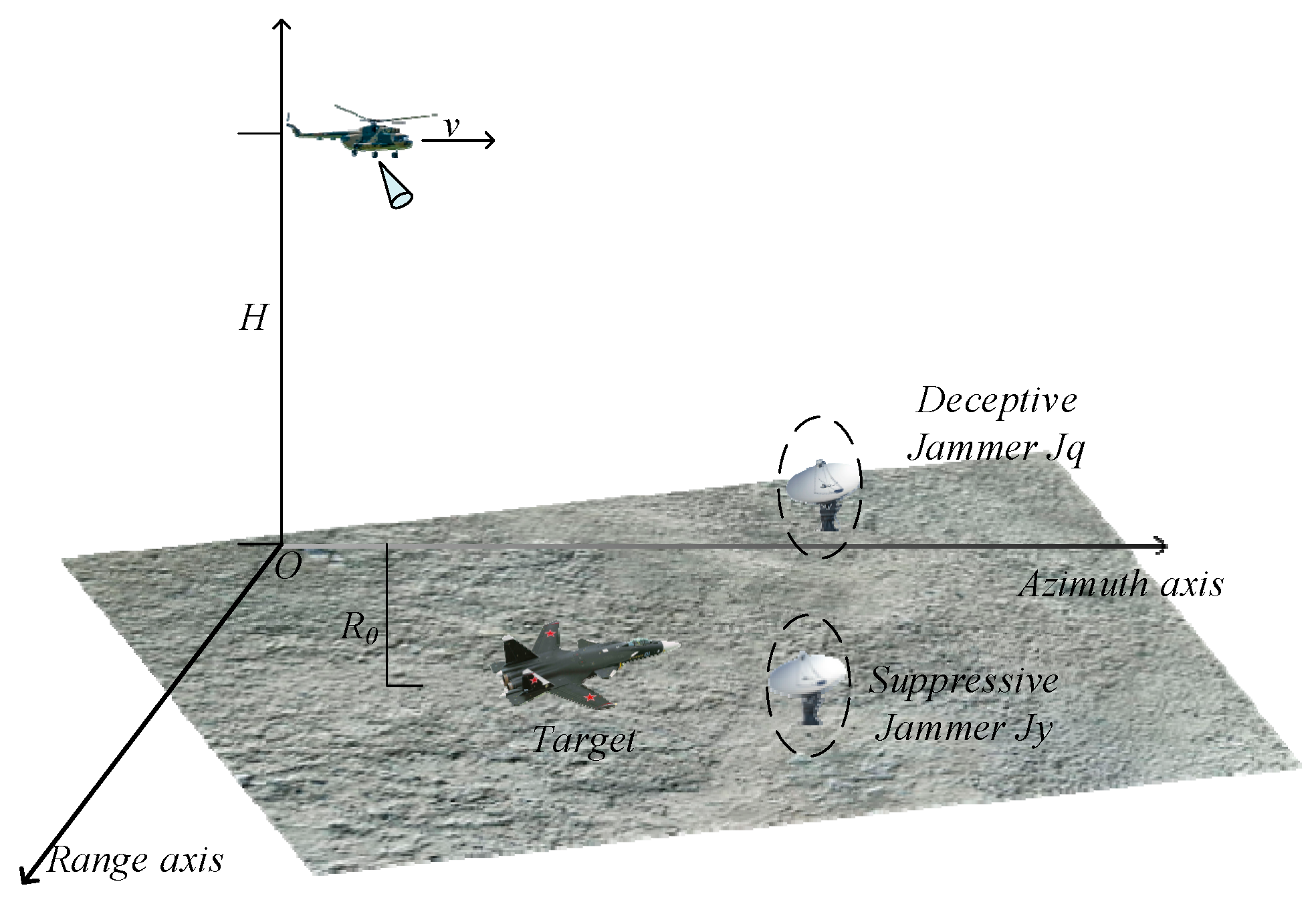
2.1. Airborne SAR Imaging and Signal Model

Airborne SAR geometric model imaging in a complex electromagnetic environment is displayed in Figure 1. The airborne SAR travels along the azimuth axis at the speed of $v$ and an altitude of $H$. The initial length of the ground target in the range axis is $R_0$. Surrounding the ground target are deceptive jammer $Jq$ and suppressive jammer $Jy$, which emit deceptive interference and suppressive interference, respectively, thus affecting the ground target detection behavior of the airborne SAR.

It is assumed that airborne SAR transmits a linear frequency modulation (LFM) pulse signal $s(\tau )$ which can be expressed as follows:

$$s(\tau )=\mathrm{rect}({\displaystyle \frac{\tau }{T_t}})\exp (2\pi j{f}_c\tau +\pi jk{\tau }^2)$$

(1)

where $\mathrm{rect}(·)$ is a rectangular function, and $T_t$ is the airborne SAR signal pulse width, $f_c$ is the carrier frequency of airborne SAR, $k=B_t/T$ is the signal modulation slope, $B_t$ is the airborne SAR signal bandwidth, and $\tau$ is the range axis time.

At azimuth time t, the baseband echo signal received by the airborne SAR is $s(\tau ,t)$, which can be expressed as follows:

$$\begin{array}{l}s(\tau ,t)=\mathrm{\varsigma }\mathrm{r}\mathrm{e}\mathrm{c}\mathrm{t}({\displaystyle \frac{\tau -d}{T_t}})\mathrm{rect}({\displaystyle \frac{t}{L/v}})\exp (-2\pi j{f}_{c}d)\\ \exp [\pi jk{(\tau -d)}^2]\end{array}$$

(2)

where $\mathrm{\varsigma }$ denotes the point target scattering coefficient, d is the time delay from the length between the ground objective and the airborne SAR, and L is the synthetic aperture length.

$$d={\displaystyle \frac{2\sqrt{v^2{(t-t_s)}^2+{R_0}^2+H^2}}{c}}$$

(3)

where $t_s$ is the moment when the airborne SAR is at the closest distance to the ground target and c is the light speed.

2.2. Complex Interference Signal Model

As the battlefield environment of electronic warfare becomes more and more complex, the common active interference can no longer satisfy a single interference form. Therefore, it is very necessary to study the composite jamming form of suppressive jamming and deceptive jamming, which also provides a lot of help for the electronic counter- countermeasures of modern electronic warfare. In this manuscript, we mainly study suppressive interference as noise frequency modulation interference (NFMI) and deceptive interference as frequency shift interference (FSI).

NFMI is a kind of interference in the frequency modulation of signals. The suppressive jammer first generates a sequence of Gaussian white noise such as the additive Gaussian white noise with probability density function obeying $p(x)={\displaystyle \frac{1}{\sqrt{2\pi {\mathrm{\sigma }}^2}}}\exp (-{\displaystyle \frac{{(x-\mu )}^2}{2{\mathrm{\sigma }}^2}})$. Then, the suppressive jammer generates a noisy frequency modulated signal, which is then passed through a bandpass filter to generate a bandlimited noise signal. The specific expression of NFMI is as follows:

$$J_y\left(\tau \right)=U_1\cos \left[\left(2\pi f_j\tau +2\pi k_{FM}{\displaystyle {\int }_0^t{U}_2}\left(\tau \right)d\tau \right)+{\phi }_0\right]$$

(4)

where $U_1$ is the signal amplitude, $f_j$ is the suppressive jammer carrier frequency, $k_{FM}$ denotes the frequency modulation rate, $U_2(\tau )$ is the modulated noise that obeys a Gaussian distribution, and ${\phi }_0$ is the initial phase.

FSI includes fixed frequency shift, random frequency shift, step shift, and inter-pulse segmental frequency shift interference. After receiving the radar signal, the deceptive jammer shifts the signal carrier frequency by a corresponding frequency and then forwards it. The specific expression for FSI can be expressed as follows:

$$\begin{array}{l}{J}_q(\tau ,t)={\mathrm{\varsigma }}_j\mathrm{r}\mathrm{e}\mathrm{c}\mathrm{t}({\displaystyle \frac{\tau -d}{T_t}})\mathrm{rect}({\displaystyle \frac{t}{L/v}})\exp [\pi jk{(\tau -d)}^2]\\ \exp [-2\pi j(f_j+f_d)d]\end{array}$$

(5)

where $f_d$ is the frequency shift volume and ${\mathrm{\varsigma }}_j$ is the deceptive signal amplitude.

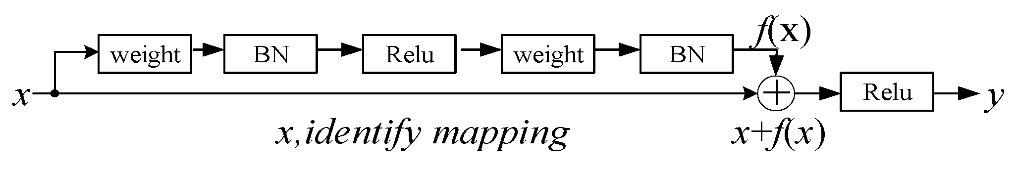
2.3. Deep Residual Learning

Significant improvements in deep learning have led to huge advances in natural language processing, image classification, and object detection [21,22,23,24,25]. The convolutional neural network (CNN) is one of the representative algorithms for deep learning, and to improve the accuracy of the CNN, the most usual method is to increase the depth of the network [26].

However, the increase in network depth leads to gradient vanishing and degradation problems [27].

ResNet solves the gradient disappearance/explosion [28,29] problem that has plagued deep learning for a long time. ResNet proposes a residual learning structure as shown in Figure 2. The basic residual module can be defined as follows:

$$y=f(x)+x$$

(6)

where y denotes the output feature sequences, x denotes the input feature sequences, and f(x) represents the residual mapping to be learned.

In a multilayer network, the output of the deeper layers can be expressed by the output of the intermediate layers, which can be expressed as follows:

$$x_L=x_l+{\displaystyle \sum _{i=l}^{L-1}F(x_i)}$$

(7)

The parameters of each layer can be transmitted throughout the network through residual learning. The gradient of the reverse process can be obtained as follows:

$${\displaystyle \frac{\partial loss}{\partial x_l}}={\displaystyle \frac{\partial loss}{\partial x_L}}{\displaystyle \frac{\partial x_L}{\partial x_l}}={\displaystyle \frac{\partial loss}{\partial x_L}}(1+{\displaystyle \frac{\partial }{\partial x_l}}{\displaystyle \sum _{i=l}^{L-1}F(x_i)})$$

(8)

The residual mapping can propagate gradients without loss, which will not lead to network degradation. And the residual gradient ${\displaystyle \frac{\partial }{\partial x_l}}{\displaystyle \sum _{i=l}^{L-1}F(x_i)}$ needs to pass through weight layers, which will not always be negative ones. Thus, the issues of vanishing gradient will not appear in the residual network.

3. Complex Electromagnetic Interference Suppression Based on BSS and the Deep Residual Network

In this section, we present a BSS algorithm using maximum kurtosis deconvolution and improved PCA for airborne SAR multi-electromagnetic interference suppression. Due to the separation uncertainty of the current BSS algorithm and the presence of residual noise, we need to identify the separated signals to obtain the target signal. Therefore, a deep residual network is proposed to solve the above problems.

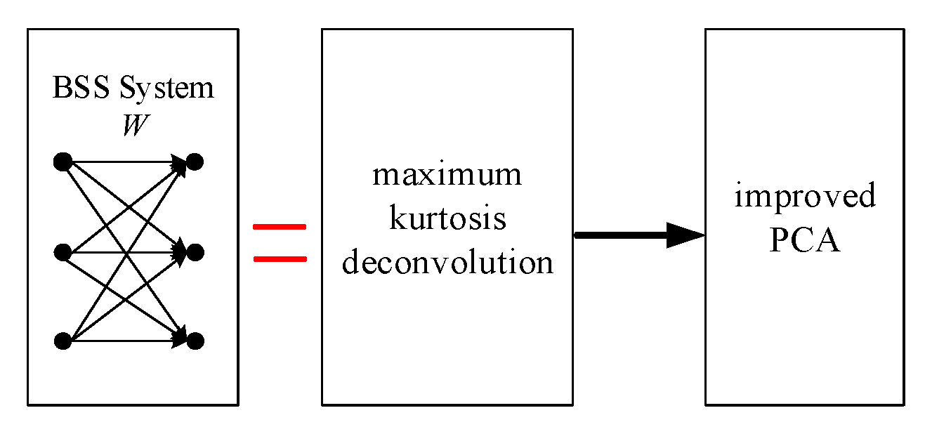
3.1. BSS Algorithm Using Maximum Kurtosis Deconvolution and Improved PCA

The BSS method can separate the target signal in the presence of the source signal and channel condition location. In this section, we propose a BSS algorithm using maximum kurtosis deconvolution and improved PCA. Assume that the target signal is $s(\tau )$, the deceptive interference signal is $J_q(\tau )$, and the suppressive interference signal is $J_y(\tau )$. After superimposing the target signal $s(\tau )$ with the noisy linear transient mixing model, we can obtain the observed signal $x(\tau )$. The noisy linear transient mixing model can be expressed as follows:

$$\left\{\begin{array}{l}{x}_1(\tau )=a_{11}s(\tau )+a_{12}{J}_y(\tau )+a_{13}{J}_q(\tau )+N\\ x_2(\tau )=a_{21}s(\tau )+a_{22}{J}_y(\tau )+a_{23}{J}_q(\tau )+N\\ x_3(\tau )=a_{31}s(\tau )+a_{32}{J}_y(\tau )+a_{33}{J}_q(\tau )+N\end{array}\right.$$

(9)

where $a_{11},a_{12},a_{13},a_{21},a_{22},a_{23},a_{31},a_{32},a_{33}$ indicates the mixing factor and $x_1(\tau )$, $x_2(\tau )$, and $x_3(\tau )$ represent the multi-channel signals of deceptive jamming signals, suppressive jamming signals, and real target signals after linear transient mixing received by the airborne SAR receiver.

The matrix form of Equation (9) can be expressed as follows:

$$x(\tau )=AQ(\tau )+N$$

(10)

where $Q(\tau )={[s(\tau ),J_y(\tau ),J_q(\tau )]}^T$, $N$ is the noise during channel transmission, ${[·]}^T$ denotes the transpose operation, and A denotes the hybrid matrix.

In order for the above Equation (10) to be solvable, we need to have the corresponding constraints and assumptions on the mixing matrix A and the source signal [30,31,32,33,34].

(1)

The mixed matrix A is the column full rank.

(2)

At most, one of the components of $Q(\tau )$ follows a Gaussian distribution.

(3)

$n(\tau )$ and $Q(\tau )$ are independent of each other.

(4)

A zero-mean random signal where the components of $Q(\tau )$ are correlated in time but not in space.

The entire flowchart of a specific BSS system is displayed in Figure 3. After superimposing the above noisy linear transient mixture model, we obtain the observation matrix $x(\tau )$.

The performance of the BSS algorithm will be greatly affected due to the presence of Gaussian white noise during channel transmission. Therefore, a denoising algorithm based on maximum kurtosis deconvolution is proposed to solve the above problem.

The maximum kurtosis deconvolution algorithm constructs the model of the system through Equation (11):

$$y(\tau )=p(\tau )\ast X(\tau )={\displaystyle \sum _{l=-\infty }^{\infty }p(l)X(\tau -l)}$$

(11)

where $p(\tau )$ is the impulse response of the system, $X(\tau )=AQ(\tau )$ represents an input impulse source, and $y(\tau )$ is the received signal which is assumed as a Toeplitz matrix.

The core idea of maximum kurtosis deconvolution is similar to finding an Nth order FIR filter. An inverse operation is performed to cancel out the effects of the convolution model so that the output after the filter can recover the input of the system. This can be described as follows:

$$\widehat{X}(\tau )={\displaystyle \sum _{\tau =0}^{N}w(l)y(\tau -l)}$$

(12)

where $w(l)$ is the inverse filter.

The kurtosis paradigm $G$ can be defined as Equation (13). According to Equation (11), Equation (13) can be written as Equation (14):

$$G(y(\tau ))={\displaystyle {\sum }_{\tau =1}^M\frac{{\left({\left|y(\tau )\right|}^2\right)}^2}{{\left(\frac{1}{M}{\displaystyle \sum _{\tau =1}^M{\left|y(\tau )\right|}^2}\right)}^2}}$$

(13)

where $M$ denotes the signal sampling number.

$$G(w(l))={\displaystyle \frac{{\displaystyle {\sum }_{\tau }\widehat{X}{(\tau )}^4}}{({\displaystyle {\sum }_{\tau }\widehat{X}{(\tau )}^2{)}^2}}}$$

(14)

By maximizing Equation (14), the optimal filter $\omega (l)$ can be obtained. According to Equation (11), Equation (15) can be obtained. The process of obtaining the optimal filter weights by maximizing the kurtosis can be represented as Equation (16):

$${\displaystyle \frac{\partial \widehat{X}(\tau )}{\partial w(l)}}=y(\tau -l)$$

(15)

$$\begin{array}{l}{\displaystyle \frac{\partial G}{\partial \omega }}=0\\ \Rightarrow G^{-1}{\displaystyle \sum _{k=1}^M{\widehat{X}}^3(\tau )y(\tau -l)}={\displaystyle \sum _{k=1}^{L}w(k){\displaystyle \sum _{k=1}^{M}y(\tau -k)}y(\tau -p)}\\ \Rightarrow G^{-1}{\displaystyle \sum _{k=1}^M{\widehat{X}}^3}T=B{\displaystyle \sum _{k=1}^{L}w(k)}\\ \Rightarrow {\displaystyle \sum _{k=1}^{L}w(k)}=B^{-1}\cdot G^{-1}{\displaystyle \sum _{k=1}^M{\widehat{X}}^3}T\end{array}$$

(16)

where T denotes the Toeplitz matrix of $y(\tau )$ and $B$ is its autocorrelation matrix, $w(k)$ is the filter coefficients updated by iteration, and $k$ represents the number of iterations.

The iterative algorithm based on maximum kurtosis inverse convolution is shown in Algorithm 1. Since the filtration factors are created by iterating, the linear phase cannot be kept.

To fix the signal phase inaccuracy, the maximum kurtosis deconvolution is improved by using the zero-phase digital filtering method, which is capable of successfully adjusting the phase delay. The mathematical idea behind it is as follows:

$$\begin{array}{l}{X}_1(\tau )=\omega (\tau )\ast y(\tau )\Rightarrow X_2(\tau )=X_1(M-\tau )\\ \Rightarrow X_3(\tau )=X(\tau )\ast X_2(\tau )\Rightarrow X(\tau )=X_3(M-\tau )\end{array}$$

(17)

With the addition of zero-phase filtering, the specific maximum kurtosis deconvolution algorithm is shown in Figure 4.

After the maximum kurtosis deconvolution algorithm proposed above, the input signal can be considered to be reduced to the correlation coefficients’ determined level. At this point, the received signal can be considered to contain only the interference and the original target signal. Next, the processed signal is separated using the proposed improved PCA algorithm. The improved PCA algorithm utilizes the combination of two PCA algorithms to transform a common signal processing problem into a simple matrix computation.

Algorithm 1 Iterative solutions for maximum kurtosis deconvolution

Step 1: Define the length N of the FIR filter $w(l)$ and the iteration stop threshold $\alpha$, initialize the filter $w(0)$

Step 2: Calculate the Toeplitz matrix X of the input signal and the autocorrelation matrix $B$

Step 3: Calculate the estimated output $\widehat{X}(k)$ based on the known output $y(k)$ and the FIR filter parameter $w(k)$

Step 4: Update $w(k+1)$ according to (16)

Step 5: Calculate the iteration error $\beta$:

$\left\{\begin{array}{c}\beta =E[(w(k+1)-\mu w(k))/\mu w(k)]\\ \mu ={(E{(w(k))}^2/E{(w(k+1))}^2)}^{1/2}\end{array}\right.$

Step 6: Stop iteration when the iteration error $\beta$ is less than the threshold $\alpha$ and the output ${\widehat{X}}_{final}=w_{best}\ast y$

In order to simplify the calculation to some extent, the improved PCA method requires the signal centering processing firstly. The specific process can be expressed as

$$\overline{x(\tau )}=x(\tau )-mean[x(\tau )]$$

(18)

where $\overline{x(\tau )}$ is the centralized processed signal and $mean(·)$ is the arithmetic mean operation.

Next, the improved PCA algorithm consists of two PCA algorithms. The improved PCA algorithm begins with a singular value decomposition (SVD) of the covariance matrix $R_x$. The specific processing can be expressed as

$$R_x=U\mathrm{\Lambda }{V}^H$$

(19)

$$W={\mathrm{\Lambda }}^{-1/2}{U}^H$$

(20)

where $R_x$ is the covariance matrix of the centralized processed signal $\overline{x(\tau )}$, W is the whitening matrix, and ${[·]}^H$ is the complex conjugate transpose operation.

$$R_x=E\left[\overline{x(\tau )}·{\overline{x(\tau )}}^H\right]={\displaystyle \frac{1}{N}}{\displaystyle \sum _{k=1}^N\overline{x(\tau )}·}{\overline{x(\tau )}}^H$$

(21)

After the first PCA, the signal $m(\tau )$ can be expressed as $m(\tau )=W\overline{x(\tau )}$. The second PCA is the process of performing the eigenvalue decomposition (EVD) of the correlation matrix $R_s$.

$$R_s\left(x\right)=E\left[m(\tau )·m{(\tau )}^H\right]={\displaystyle \frac{1}{N}}{\displaystyle \sum _{k=1}^{N}m(\tau )·m{(\tau -x)}^H}$$

(22)

The specific processing can be expressed as follows:

$$R_s(1)=C\mathrm{\Lambda }{C}^H$$

(23)

$$S=C$$

(24)

where $R_s(1)$ is the correlation matrix whose delay is one and $S$ is the separation matrix.

Finally, we can obtain the estimated signal $x^{\prime }(\tau )$

$$x^{\prime }(\tau )=Sm(\tau )=C^H{\mathrm{\Lambda }}^{-1/2}{U}^H\overline{x(\tau )}$$

(25)

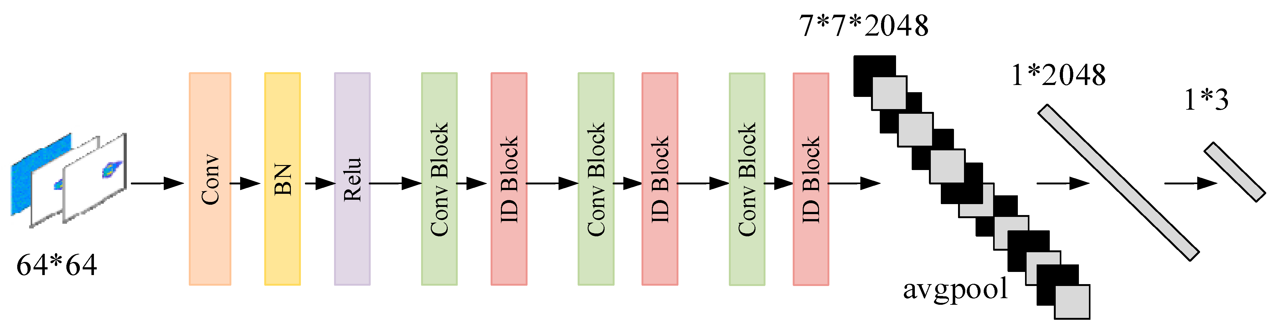
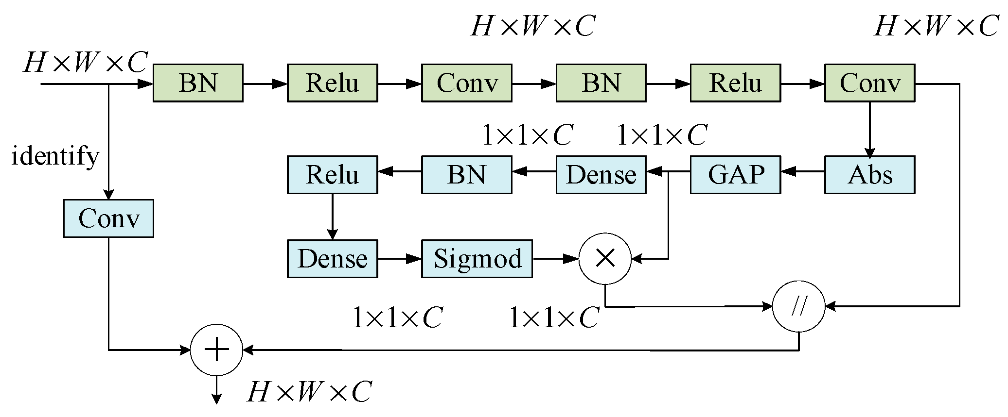
3.2. Signal Recognition Based on the Deep Residual Network

After the proposed BSS approach above, we encountered the problem of uncertainty in the order of separation. Similarly, due to the presence of Gaussian white noise during channel transmission, the separated signal still had residual noise. We had difficulty distinguishing which signal was being separated. Thus, how to identify the separated signals after the BSS method is a very important question.

Prior to signal identification, we need to perform airborne SAR imaging of the separated signals. Common SAR imaging methods include the range Doppler (RD) imaging method, the backward projection (BP) imaging method, the chirp scaling (CS) imaging method, and so on. In this manuscript, the airborne SAR imaging algorithm that we use is the classical RD imaging algorithm.

To address the problems that arise above, the authors of reference [35] propose the use of support vector machines (SVMs) and PCA methods for signal identification. The traditional classifier approach described above suffers from the difficulty of feature extraction. In this section, a deep residual network [36,37] is proposed to recognize the separated signals.

The authors of reference [38] use algorithmic unfolding to unfold iterative algorithms into deep networks, making the design and optimization process of the network more transparent. A network called BM3D-Net is proposed in the literature [39]. BM3D-Net is effective in removing image noise and preserving image details in terms of collaborative filtering in the transform domain. Although the iterative algorithm can reduce the complexity of network computation and BM3D-Net can effectively remove noise, the iterative algorithm has poor generalization ability, and BM3D-Net has a narrow range of applications. Therefore, we propose a deep residual network. It can not only achieve image denoising, but also has strong generalization ability and is simple to implement.

Since the above proposed BSS method is performed in a noisy environment, residual noise can easily exist in the separated signal. In order to address the effects of residual noise, a residual shrinkage structure is proposed for noise suppression.

The residual shrinkage network [40] takes advantage of the residual learning ability and the soft threshold. The block diagram of the residual shrinkage module is shown in Figure 5. In Figure 6, BN represents the batch normalization operation, Abs represents the modulo value, Relu [41] and Sigmoid represent the activation function, GAP represents global average pooling, Dense means the multilayer perceptron, and Conv is the convolutional operation. From Figure 6, it is easy to find that the residual shrinkage network includes a shortcut connection that can skip one or more layers.

The diagram of the proposed deep residual network is shown in Figure 5. In Figure 5, the airborne SAR images generated by the separated signals will first go through the Convolution operation, the BN operation, and the Relu operation. Then, six residual shrinkage modules are used sequentially to extract image features. When there exists a convolution operation in the basic residual module of the residual shrinkage block, the residual shrinkage block is defined as the Conv Block. Otherwise, the residual shrinkage block is defined as the ID Block. Multiple feature extraction layers ensure fine image feature extraction. At the same time, the training parameters of each weight layer are transmitted through the basic residual module. In order to reduce the dimensionality of the network output features, a global average pooling layer is added at the end of the feature capture layer. Lastly, the features are sent to the multilayer perceptron to train the classification network. The output of the networks is the recognition results. It is easy to obtain the target signal through the recognition results.

3.3. Summary of the Entire Method

The overall flowchart of the proposed algorithm is shown in Figure 7. The entire algorithm consists of two parts: the BSS method and the deep residual network. The target signal and the interference signal first enter the BSS system through a noisy linear instantaneous mixing model. The BSS system mainly includes two parts: maximum kurtosis deconvolution and the improved PCA. Through the maximum kurtosis deconvolution algorithm, the existence of Gaussian white noise in the process of channel transmission can be removed. Through the improved PCA algorithm, the separated signals can be obtained using a simple matrix computation method. Through the above steps, the BSS methodology is accomplished.

At the same time, the existing BSS algorithm still has the problem of separation order uncertainty. Next, in order to solve the above problems, the separated signals are identified through the proposed deep residual network. Finally, according to the classification result of the recognition module, the target signal can be obtained.

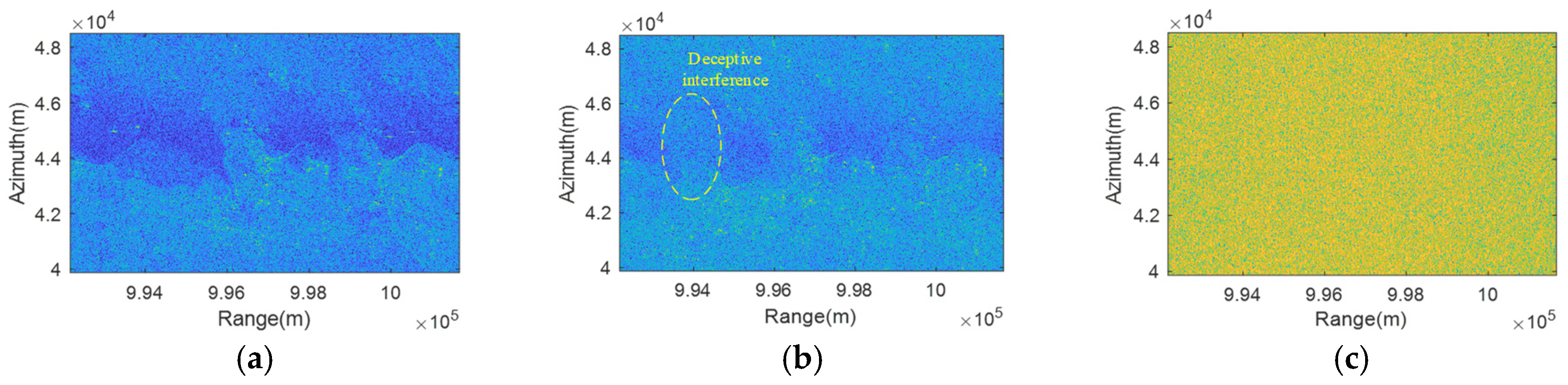
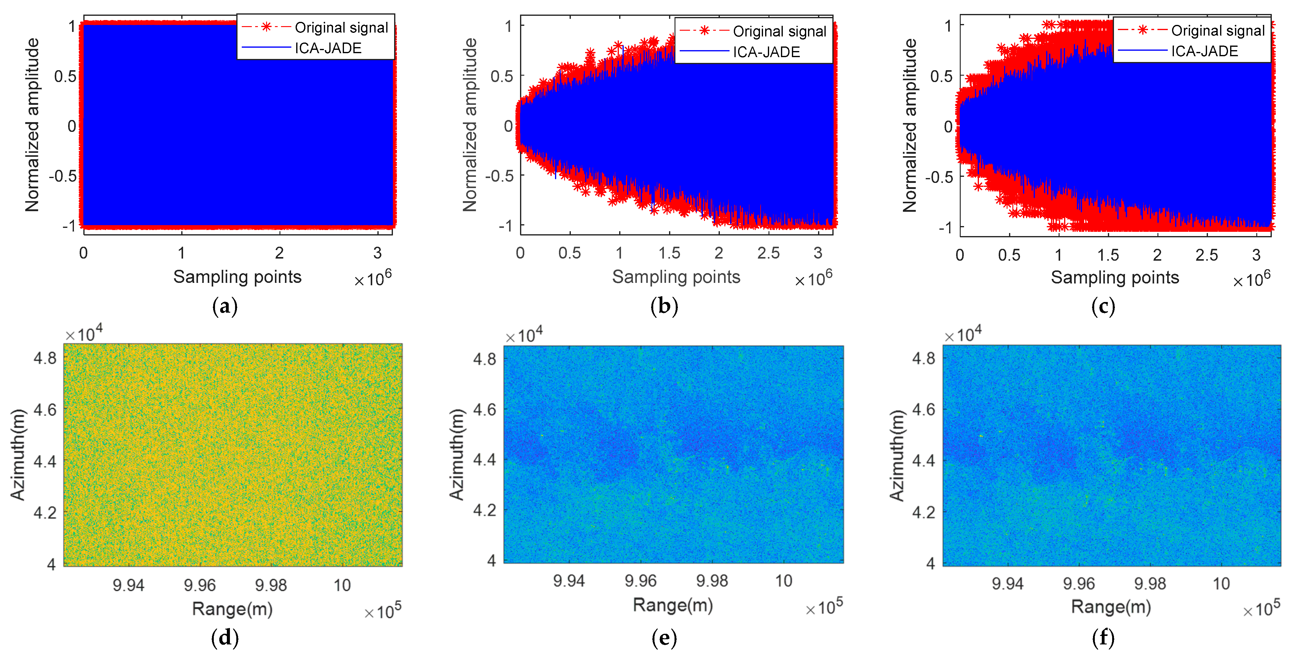
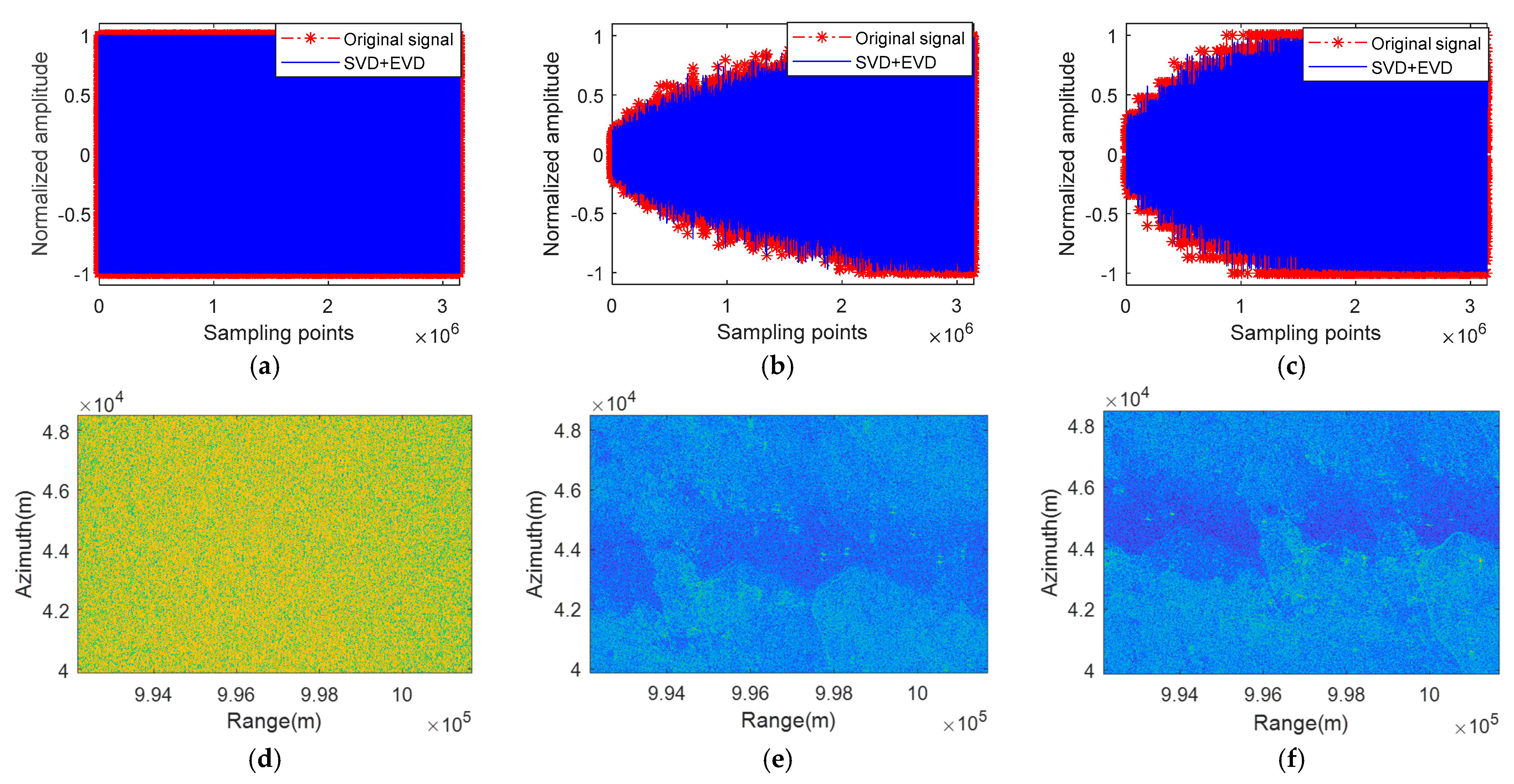
4. Experimental Results and Analysis

In Section 3, a complex electromagnetic interference suppression method based on the BSS method and a deep residual network is proposed.

The authors of reference [42] propose an independent component analysis (ICA) algorithm using joint approximate diagonalization of eigenmatrices (JADEs) to suppress narrowband suppressive interference. The authors of reference [43] propose a BSS algorithm using SVD and EVD to suppress suppressive interference. To further validate the effectiveness of our proposed algorithm, we compare our proposed algorithm with the ICA-JADE algorithm and the SVD + EVD algorithm and demonstrate the behavior of our presented algorithm using both simulation and measurement exeriments.

4.1. Evaluation Criteria

In order to quantitatively characterize the performance of the proposed algorithm for complex electromagnetic jamming suppression, we propose two quantitative evaluation criteria. The two evaluation criteria are the signal correlation coefficient (SCC) and the picture root mean square error (PMSE).

The SCC is a measure of how similar the signal is before and after complex electromagnetic interference suppression. The formula of SCC can be expressed as follows:

$$\mathrm{SCC}={\displaystyle \frac{{\displaystyle \sum _{n=1}^{Na\ast N_r}[x(\tau )-\overline{x(\tau )}]}[x^{\prime }(\tau )-\overline{x^{\prime }(\tau )}]}{\sqrt{{\displaystyle \sum _{n=1}^{Na\ast N_r}{[x(\tau )-\overline{x(\tau )}]}^2}}\sqrt{{\displaystyle \sum _{n=1}^{Na\ast N_r}{[x^{\prime }(\tau )-\overline{x^{\prime }(\tau )}]}^2}}}}$$

(26)

where Na is the azimuth sampling points, Nr is the range sampling points, $x(\tau )$ is the original signal before complex electromagnetic interference, and $\overline{·}$ is the mean value calculation method.

PMSE is a metric for measuring image error before and after complex electromagnetic interference suppression. The formula of PMSE can be expressed as follows:

$$\mathrm{PMSE}=10\ast \lg \left\{{\displaystyle \frac{1}{ab}}\right.{\displaystyle \sum _{x=0}^{a-1}{\displaystyle \sum _{y=0}^{b-1}\left|\right|}}M\left(x,y\right)-N\left(x,y\right)\left.|{|}^2\right\}$$

(27)

where a is the row number, b is the column number, $M\left(x,y\right)$ is the grayscale of the picture before complex electromagnetic interference suppression, and $N\left(x,y\right)$ is the grayscale of the picture after complex electromagnetic interference suppression.

4.2. Simulation Experiments and Analysis

In this part, the simulation experiments are used to compare and analyze the performance of our proposed method for the suppression of complex electromagnetic interference.

The simulated parameters for suppressive interference and deceptive interference, and the airborne SAR targets are shown in

Table 1. Simulated parameters.

Settings	Size	Settings	Size
Central frequency	1.5 (GHz)	Pulse width	1.5 (μs)
Signal bandwidth	150 (MHz)	SAR height	1000 (m)
Speed of SAR	100 (m/s)	The SNR of noise	10 (dB)
Range samples	1024	Suppressive interference frequency	1.5 (GHz)
Azimuth samples	1024	Suppressive interference bandwidth	450 (MHz)
SJR of FSI	0 (dB)	Azimuth frequency shift	45 (MHz)
SJR of NFMI	−35 (dB)	Range frequency shift	60 (MHz)

. In the simulation experiments, the suppressive interference used is the NFMI mentioned above, and the deceptive interference used is the FSI mentioned above. For NFMI, the interference bandwidth is set to be three times the signal bandwidth because it uses a large bandwidth and high power signal to cover the original signal to form a suppression effect. In this experiment, the signal bandwidth is set to 150 MHz, the suppressive interference is set to 450 MHz. For FSI, since it is obtained by frequency shifting the original signal after it is intercepted by a deceptive jammer, it is usually azimuth shifted and range shifted. In this experiment, the azimuth frequency shift is set to 60 MHz, and the range frequency shift is set to 495 MHz so that a deceptive jamming false target can be generated near the real target. Since the signal is noisy during transmission, the signal-to-noise ratio is set to 10 dB in this simulation experiment.

The airborne SAR imaging results of the simulation experiment are displayed in Figure 8. The simulation target is an aircraft. The results of deceptive jamming are displayed in Figure 8b, and the results of combined deceptive and suppressive jamming are displayed in Figure 8c. From Figure 8, it is easy to see that the target generated by deceptive jamming is extremely similar to the real target, and it is difficult to detect the real target and the target generated by deceptive jamming after the suppressive jamming is added.

With the above description, the received signals include the original target signal, suppressive interference, and deceptive interference. Therefore, the results of the simulation experiments mainly include suppressive interference, deceptive interference, original target signal. In order to compare our proposed method with the other algorithms, the experimental results are simulated from the point of view of the signal and the SAR image.

Figure 9 demonstrates the results of the ICA-JADE algorithm after complex electromagnetic interference suppression. Figure 10 shows the results of the SVD + EVD algorithm after complex electromagnetic interference suppression. Figure 11 shows the results of our proposed algorithm after complex electromagnetic interference suppression. After comparing the complex electromagnetic interference results of our proposed algorithm with the complex electromagnetic interference results of the ICA-JADE algorithm and the SVD + EVD algorithm, some conclusions were reached.

From the perspective of the airborne SAR images of the suppressive jamming and the suppressive jamming after the suppression of the complex electromagnetic jamming, it is easy to find that by comparing our proposed algorithm with the ICA-JADE algorithm and the SVD + EVD algorithm, they all have great recovery performance for suppressive interference signals compared to each other. However, it is difficult to judge the texture characteristics of the suppressive interference image with the naked eye.

From the perspective of the airborne SAR images of the deceptive jamming and the deceptive jamming after the suppression of the complex electromagnetic interference, it is easy to find that the ICA-JADE algorithm has greater signal loss after the complex electromagnetic interference suppression compared to our proposed algorithm, and it is difficult to separate the target signal from the deceptive interference signal on the airborne SAR images of the signals after the complex electromagnetic interference suppression. However, although the SVD + EVD algorithm has less signal loss, there is still a small amount of target signal residue in the airborne SAR image generated by the deceptive interference signal after complex electromagnetic interference suppression.

From the perspective of the airborne SAR images of the original signal and the original signal after the suppression of the complex electromagnetic interference, it is easy to find that the ICA-JADE algorithm still has deceptive jamming signals on the image of the original signal, and the ICA-JADE method recovers a greater loss of signal. The SVD + EVD algorithm and our proposed algorithm can all recover the target signal. It is hard to distinguish the airborne SAR images of the original signal after the suppression of the complex electromagnetic interference using the SVD + EVD algorithm and our proposed algorithm with the naked eye. Both methods can recover the airborne SAR images of the original signal.

Through the above elaboration, it is difficult to fully distinguish the advantages of our proposed algorithm over the SVD + EVD algorithm with only the naked eye. To address this issue, the evaluation criteria values were calculated. The specific values of the evaluation criteria in the simulation experiment are shown in

Table 2. Evaluation criteria of simulation experiments.

Evaluation Criteria		ICA-JADE	SVD + EVD	Ours
SCC	Suppressive interference	1	1	1
	Deceptive interference	0.6484	0.9717	1
	Original signal	0.5931	0.9890	1
PMSE (dB)	Suppressive interference	−14.9876	−15.5805	−15.7228
	Deceptive interference	−38.5028	−52.1302	−112.1117
	Original signal	−41.9832	−80.0315	−125.2649

. By observing the data in Table 2, we can see that the ICA-JADE method, the SVD + EVD method, and our proposed method have good SCC in suppressive interference recovery.

In addition, our proposed algorithm has better performance than the ICA-JADE algorithm and the SVD + EVD algorithm in terms of complex electromagnetic interference suppression. Our proposed algorithm has better SCC and lower PMSE compared with the ICA-JADE method and the SVD + EVD algorithm.

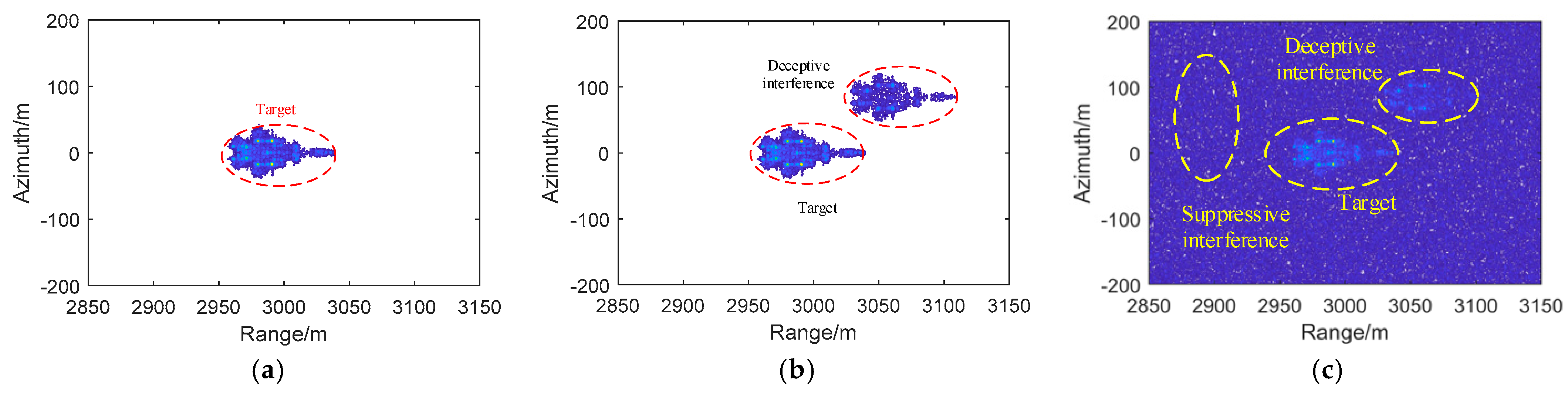
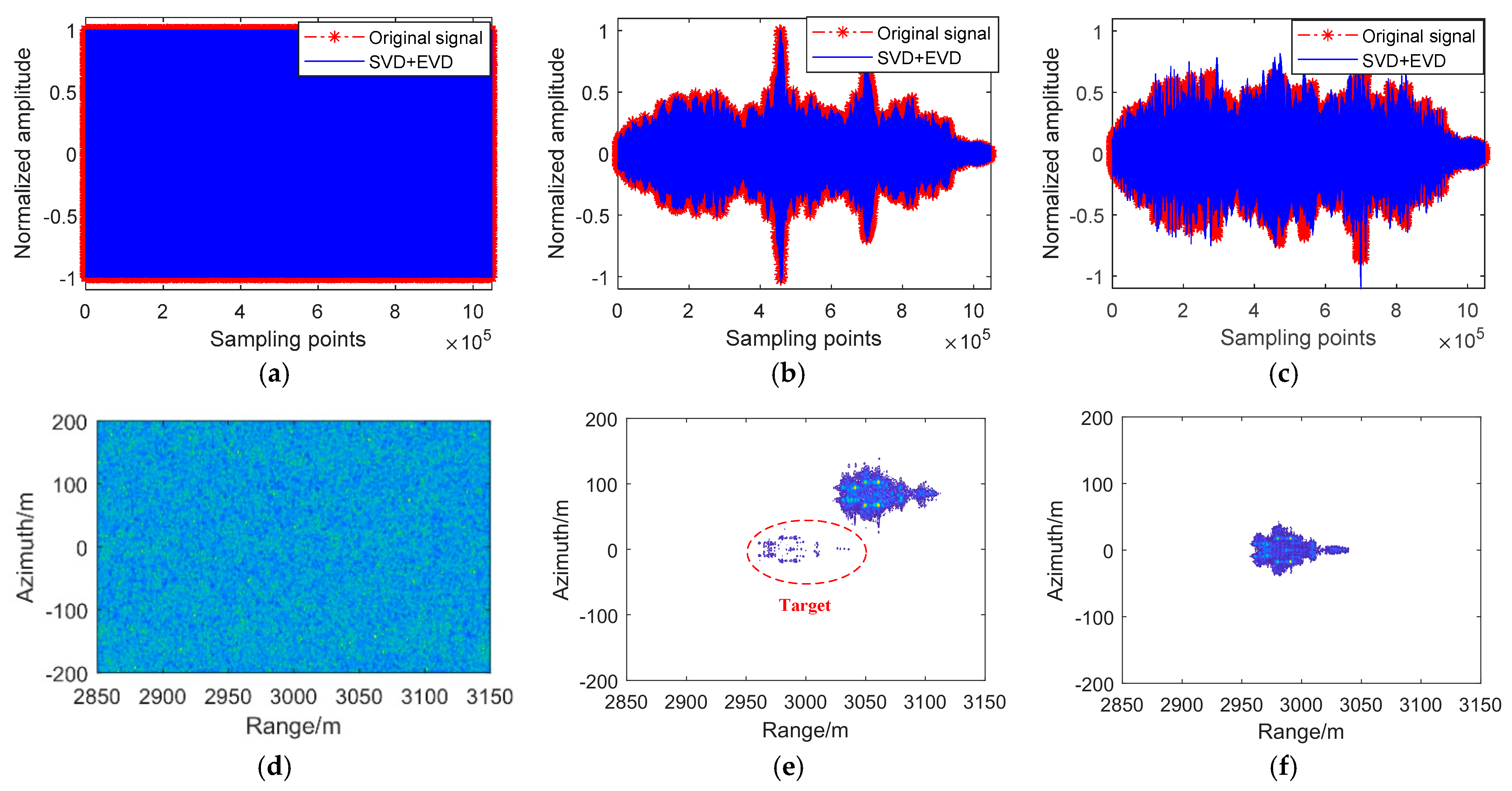
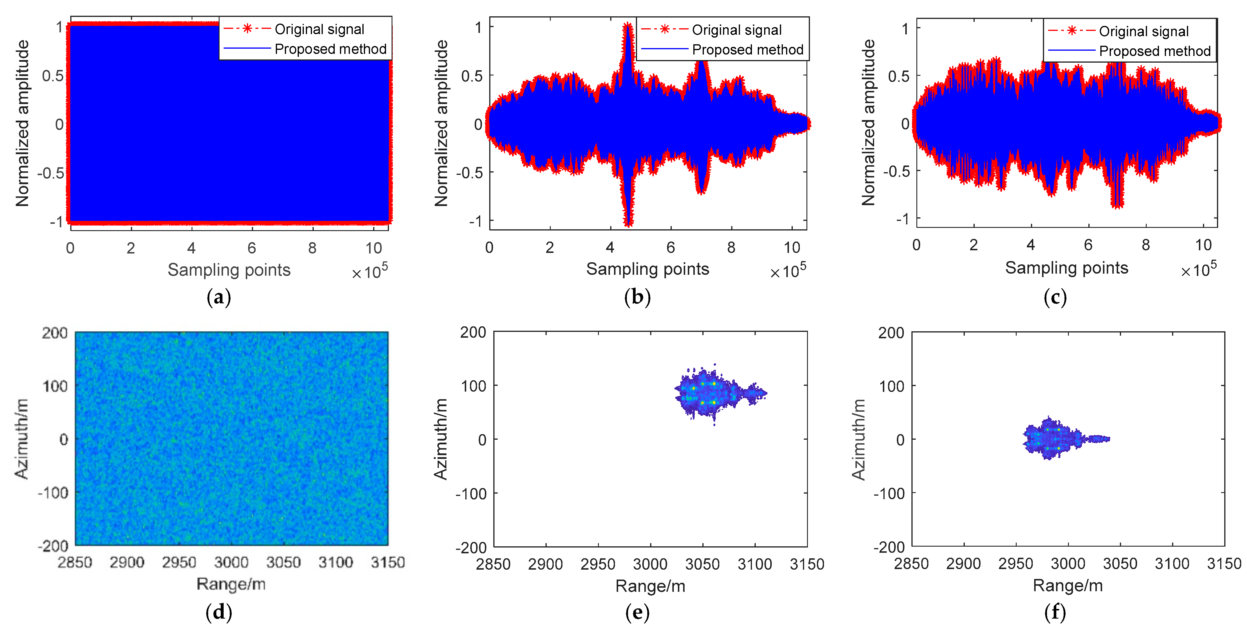
4.3. Measurement Experiments and Analysis

To further verify the behavior of our proposed method for complex electromagnetic interference suppression, a comparative analysis was carried out using the measured data of RADARSAT-1 transmitted by the Canadian Space Agency.

In this RADARSAT-1 experiment, since the data of RADARSAT-1 are publicly available, we can know its signal bandwidth and signal form. When the central frequency of the suppressive interference is in the same band as this RADARSAT-1 signal, the radar receiver can receive the interference, and at this time, the entire experiment is considered to be completed. Similarly, since the signal is publicly known, deceptive interference is created by frequency shifting the signal. Suppressive interference, on the other hand, is generated by simulating a noise sequence, utilizing modulation techniques to create the interference, and finally adding it to the RADARSAT-1 data through an additive model. In this experiment, the range frequency shift of the frequency-shifted interference was set to 0.4Br, and the azimuth frequency shift was set to 0.3Br, where Br represents the signal bandwidth of the RADARSAT-1 data.

The imaging results of the measurement experiment are displayed in Figure 12. The target imaging area is the harbor and a few ships. The results of deceptive jamming are shown in Figure 12b, and the results of combined deceptive and suppressive jamming are displayed in Figure 12c. From Figure 12, it is easy to see that the SAR image generated by deceptive jamming is extremely similar to the SAR image generated by the real echo signal, and it is difficult to detect the real echo signal and deceptive jamming after suppressive jamming is added.

Figure 13 demonstrates the results of the ICA-JADE algorithm after complex electromagnetic interference suppression. Figure 14 demonstrates the results of the SVD + EVD method after complex electromagnetic interference suppression. Figure 15 demonstrates the results of our proposed method after complex electromagnetic interference suppression. After observing and comparing the complex electromagnetic interference results of our proposed algorithm with the complex electromagnetic interference results of the ICA-JADE algorithm and the SVD + EVD algorithm in Figure 13, Figure 14 and Figure 15, some conclusions can be drawn.

Comparing the restored suppressive interference signals after complex electromagnetic interference suppression using the ICA-JADE algorithm, the SVD + EVD algorithm, and our proposed algorithm, we can see that all of the algorithms have good restoration performance for suppressive interference, and the similarity of the SAR images is high, with specific textural differences difficult to distinguish directly.

Comparing the restored deceptive interference signals after complex electromagnetic interference suppression using the ICA-JADE method, the SVD + EVD algorithm, and our proposed method, we can see that the signal loss restored using the ICA-JADE method is greater, and the SAR image restored using the ICA-JADE method still has a residual target signal image. Both the SVD + EVD algorithm and our proposed algorithm can recover the deceptive interference signal well. However, compared to our proposed algorithm, there is still a small amount of interference in the deceptive interference images recovered by the SVD + EVD algorithm.

Comparing the restored original signals after complex electromagnetic interference suppression using the ICA-JADE method and our proposed method, we can see that the signal loss restored using the ICA-JADE method is greater, and the SAR image restored using the ICA-JADE method still has a deceptive interference signal image. Both the SVD + EVD algorithm and our proposed algorithm can recover the original signal well. However, compared to our proposed algorithm, there is still a small amount of interference in the original signal images recovered using the SVD + EVD algorithm.

Through the above elaboration, it is difficult to fully distinguish the advantages of our proposed algorithm over the SVD + EVD algorithm with only the naked eye. To address this issue, the evaluation criteria values were calculated. The specific values of the evaluation criteria in the measurement experiments are displayed in

Table 3. Evaluation criteria of measurement experiments.

Evaluation Criteria		ICA-JADE	SVD + EVD	Ours
SCC	Suppressive interference	1	1	1
	Deceptive interference	0.6796	0.9996	1
	Original signal	0.6941	0.9993	1
PMSE (dB)	Suppressive interference	−14.8063	−15.7655	−16.4375
	Deceptive interference	−22.0090	−78.2647	−88.5516
	Original signal	−23.4203	−83.5666	−88.1238

. By observing the data in Table 3, it is easy to find that the ICA-JADE method, the SVD + EVD algorithm, and our proposed method have good SCC in suppressive interference recovery. In addition, our proposed algorithm has better performance than the ICA-JADE algorithm and the SVD + EVD algorithm in terms of complex electromagnetic interference suppression. Our proposed algorithm has better SCC and lower PMSE compared with the ICA-JADE method and the SVD + EVD algorithm.

Combining the simulation and measurement results, our proposed algorithm has good recovery of suppressive interference signals, deceptive interference signals, and the original target signals. However, while the ICA-JADE method is good at recovering suppressive interference signals, it has difficulty in recovering deceptive interference signals and the original target signals. Similarly, although the SVD + EVD algorithm already has good complex electromagnetic interference suppression performance, our proposed method maintains certain advantages in both image recovery and signal recovery.

4.4. Overall Recognition Results for Deep Residual Networks

Deep learning tools are widely used in real life today and can be used to solve many problems. The authors of reference [38] propose an efficient deep learning means for signal and image processing. The authors of [39] propose a convolutional neural network for transform-domain collaborative filtering called BM3D-Net. The authors of [44] propose the ResNet network, he authors of [45] propose the AlexNet network, the authors of [46] propose the VGGNet network, and the authors of [47] propose the GoogLeNet network.

In order to validate the feasibility and effectiveness of the proposed deep residual network, a comparative analysis with AlexNet, VGGNet, Resnet, and GoogLeNet was performed.

After processing using the BSS separation method, the recovered signal contains multiple components, and for anti-interference purposes, we need to identify the recovered original target signal among the multiple recovered signals. Therefore, in this phase, the identification task is centered on identifying the recovered real target signal from the recovered suppressive jamming, deceptive jamming, and the real target. The specific recognition rate represents the performance of this network.

We acquired the SAR images of the separated signals in the presence of suppressive interference with different signal-to-jamming ratios (SJRs). The dataset generated from the separated signals was then acquired using the classical RD imaging algorithm.

The total number of experiments is 300, and the total number of images is 900, of which 810 images are used as the training set data and 90 images are used as the validation set data. We trained four epochs separately and experimented 10 times in total. We used a personal computer (PC) with an NVIDIA GeForce RTX 3050 graphics card, a memory of 64 GB, and a 13th Gen Intel(R) Core (TM) i5-13600KF CPU for training. Since the training sample is not particularly large, we used the CPU for training.

The overall recognition results of the simulation experiments are presented in

Table 4. Overall recognition rate of simulation experiments.

Network	Overall Recognition Rate
AlexNet	84.3%
VGGNet	87.2%
ResNet	94.3%
GoogLeNet	94.2%
Ours	95.7%

, while the recognition outcomes from the measurement experiments are summarized in

Table 5. Overall recognition rate of measurement experiments.

Network	Overall Recognition Rate
AlexNet	93.2%
VGGNet	92.2%
ResNet	95.3%
GoogLeNet	96.9%
Ours	99.6%

. As evidenced by the data in Table 4 and Table 5, our proposed method, along with ResNet and GoogLeNet, demonstrates significantly enhanced classification performance compared to AlexNet and VGGNet, primarily attributed to the residual structure that effectively mitigates gradient vanishing issues. Furthermore, compared to ResNet and GoogLeNet, our contraction network incorporates an additional soft thresholding filtering module. This architectural enhancement achieves an accuracy improvement of approximately 1.5% in simulated data and nearly 3% in measured data, while incurring negligible computational overhead. These findings collectively demonstrate that our proposed deep residual network exhibits superior reliability in identifying signals separated using BSS methods.

5. Conclusions

In this manuscript, an algorithm using BSS and a deep residual network is presented to suppress complex electromagnetic interference for airborne SAR. Firstly, the signal mixed model and the geometric imaging model under complex electromagnetic interference conditions are proposed. Next, a BSS algorithm using maximum kurtosis deconvolution and improved PCA is presented. To address the problem of the separation order uncertainty performance of the BSS method and the existence of noise, a deep residual network is designed to solve the above existential problems. The results of the simulations and measurement experiments demonstrate that our presented algorithm has a good performance on both SCC and PMSE, with better complex electromagnetic jamming suppression performance compared to the ICA-JADE algorithm and the SVD + EVD algorithm. Similarly, the proposed deep residual network gives better overall recognition results than the traditional networks in both the simulations and measurement experiments.

References

1. Bai, X.; Zhou, F.; Xing, M.; Bao, Z. Scaling the 3-D Image of Spinning Space Debris via Bistatic Inverse Synthetic Aperture Radar. IEEE Geosci. Remote Sens. Lett. 2010, 7, 430–434. [Google Scholar] [CrossRef]
2. Soumekh, M. Moving target detection in foliage using along track monopulse synthetic aperture radar imaging. IEEE Trans. Image Process. 1997, 6, 1148–1163. [Google Scholar] [CrossRef]
3. Fortuny, J.; Sieber, A. Three-dimensional synthetic aperture radar imaging of a fir tree: First results. IEEE Trans. Geosci. Remote Sens. 1999, 37, 1006–1014. [Google Scholar] [CrossRef]
4. Li, Z.; Wang, J.; Liu, Q.H. Frequency-Domain Backprojection Algorithm for Synthetic Aperture Radar Imaging. IEEE Geosci. Remote Sens. Lett. 2015, 12, 905–909. [Google Scholar]
5. Zhang, X.; Liu, Z.; Kong, Y.; Li, C. Mutual Interference Suppression Using Signal Separation and Adaptive Mode Decomposition in Noncontact Vital Sign Measurements. IEEE Trans. Instrum. Meas. 2022, 71, 4001015. [Google Scholar] [CrossRef]
6. Reverter, F.; Gasulla, M.; Pallas-Areny, R. Analysis of Power-Supply Interference Effects on Direct Sensor-to-Microcontroller Interfaces. IEEE Trans. Instrum. Meas. 2007, 56, 171–177. [Google Scholar] [CrossRef]
7. Cadambe, V.R.; Jafar, S.A. Interference Alignment and Degrees of Freedom of the K-User Interference Channel. IEEE Trans. Inf. Theory. 2008, 54, 3425–3441. [Google Scholar] [CrossRef]
8. Popescu, D.C.; Yaddanapudi, P. Narrowband Interference Avoidance in OFDM-Based UWB Communication Systems. IEEE Trans. Commun. 2007, 55, 1667–1673. [Google Scholar] [CrossRef]
9. Nie, G.; Liao, G.; Zeng, C.; Zhang, X.; Li, D. Joint Radio Frequency Interference and Deceptive Jamming Suppression Method for Single-Channel SAR via Subpulse Coding. IEEE J. Sel. Top. Appl. Earth Obs. Remote Sens. 2023, 16, 787–798. [Google Scholar] [CrossRef]
10. Liao, Y.; Tang, H.; Wang, W.-Q.; Xing, M. A Low Sidelobe Deceptive Jamming Suppression Beamforming Method with a Frequency Diverse Array. IEEE Trans. Antennas Propag. 2022, 70, 4884–4889. [Google Scholar] [CrossRef]
11. Huang, Y.; Zhang, L.; Li, J.; Chen, Z.; Yang, X. Reweighted Tensor Factorization Method for SAR Narrowband and Wideband Interference Mitigation Using Smoothing Multiview Tensor Model. IEEE Trans. Geosci. Remote Sens. 2020, 58, 3298–3313. [Google Scholar] [CrossRef]
12. Zhang, W.; Tait, A.; Huang, C.; Ferreira de Lima, T.; Bilodeau, S.; Blow, E.C.; Jha, A.; Shastri, B.J.; Prucnal, P. Broadband physical layer cognitive radio with an integrated photonic processor for blind source separation. Nat. Commun. 2023, 14, 1107. [Google Scholar] [CrossRef] [PubMed]
13. Chang, S.; Deng, Y.; Zhang, Y.; Zhao, Q.; Wang, R.; Zhang, K. An Advanced Scheme for Range Ambiguity Suppression of Spaceborne SAR Based on Blind Source Separation. IEEE Trans. Geosci. Remote Sens. 2022, 60, 5230112. [Google Scholar] [CrossRef]
14. Brendel, A.; Haubner, T.; Kellermann, W. A Unifying View on Blind Source Separation of Convolutive Mixtures Based on Independent Component Analysis. IEEE Trans. Signal Process. 2023, 71, 816–830. [Google Scholar] [CrossRef]
15. Herault, J.; Jutten, C. Space or time adaptive signal processing by neural network models. In Proceedings of the AIP Conference Proceedings, Snowbird, UT, USA, 13–16 April 1986; Volume 151, pp. 206–211. [Google Scholar]
16. Giannakis, G.B.; Swami, A. New Results On State-Space And Input-Output Identification Of Non-Gaussian Processes Using Cumulants. In Advanced Algorithms and Architectures for Signal Processing II, Proceedings of the 31st Annual Technical Symposium on Optical and Optoelectronic Applied Sciences and Engineering, San Diego, CA, USA, 21 January 1988; International Society for Optics and Photonics: Bellingham, WA, USA, 1988. [Google Scholar]
17. Jutten, C.; Herault, J. Blind separation of sources, part I: An adaptive algorithm based on neuromimetic architecture. Signal Process. 1991, 24, 1–10. [Google Scholar] [CrossRef]
18. Dutta, S.; Basarab, A.; Georgeot, B.; Kouamé, D. A novel image denoising algorithm using concepts of quantum many-body theory. Signal Process. 2022, 201, 108690. [Google Scholar] [CrossRef]
19. Chen, Y.K.; Bakhary, N.; Padil, K.H.; Li, J.; Shamsudin, M.F. Reducing false damage detections in guided ultrasonic wave monitoring systems using a denoising autoencoder. Nondestruct. Test. Eval. 2024, 40, 1610–1640. [Google Scholar] [CrossRef]
20. Sophian, A.; Tian, G.Y.; Taylor, D.; Rudlin, J. A feature extraction technique based on principal component analysis for pulsed Eddy current NDT. NDT E Int. 2003, 36, 37–41. [Google Scholar] [CrossRef]
21. Chen, K.; Wang, L.; Zhang, J.; Chen, S.; Zhang, S. Semantic Learning for Analysis of Overlapping LPI Radar Signals. IEEE Trans. Instrum. Meas. 2023, 72, 8501615. [Google Scholar] [CrossRef]
22. Sarikaya, R.; Hinton, G.E.; Deoras, A. Application of Deep Belief Networks for Natural Language Understanding. IEEE/ACM Trans. Audio Speech Lang. Process. 2014, 22, 778–784. [Google Scholar] [CrossRef]
23. Fan, J.; Zhao, T.; Kuang, Z.; Zheng, Y.; Zhang, J.; Yu, J.; Peng, J. HD-MTL: Hierarchical Deep Multi-Task Learning for Large-Scale Visual Recognition. IEEE Trans. Image Process. 2017, 26, 1923–1938. [Google Scholar] [CrossRef] [PubMed]
24. Li, H.; Lin, Z.; Shen, X.; Brandt, J.; Hua, G. A Convolutional Neural Network Cascade for Face Detection. In Proceedings of the 2015 IEEE Conference on Computer Vision and Pattern Recognition (CVPR), Boston, MA, USA, 12 June 2015; pp. 5325–5334. [Google Scholar]
25. Meng, Z.; Zhang, M.; Wang, H. CNN with Pose Segmentation for Suspicious Object Detection in MMW Security Images. Sensors 2020, 20, 4974. [Google Scholar] [CrossRef]
26. Zeiler, M.D.; Fergus, R. Visualizing and Understanding Convolutional Networks. In Proceedings of the European Conference on Computer Vision, New York, NY, USA, 6–12 September 2014; Springer: Princeton, NJ, USA, 2014; pp. 818–833. [Google Scholar]
27. Russakovsky, O.; Deng, J.; Su, H.; Krause, J.; Satheesh, S.; Ma, S.; Huang, Z.; Karpathy, A.; Khosla, A.; Bernstein, M.; et al. ImageNet Large Scale Visual Recognition Challenge. Int. J. Comput. Vis. 2015, 115, 211–252. [Google Scholar] [CrossRef]
28. Bengio, Y.; Simard, P.; Frasconi, P. Learning long-term dependencies with gradient descent is difficult. IEEE Trans. Neural Netw. 1994, 5, 157–166. [Google Scholar] [CrossRef]
29. Glorot, X.; Bengio, Y. Understanding the difficulty of training deep feedforward neural networks. In Proceedings of the Thirteenth International Conference on Artificial Intelligence and Statistics, Sardinia, Italy, 13–15 May 2010; JMLR Workshop and Conference Proceedings. pp. 249–256. [Google Scholar]
30. Belouchrani, A.; Abed-Meraim, K.; Cardoso, J.F.; Moulines, E. A blind source separation technique using second-order statistics. IEEE Trans. Signal Process. 1997, 45, 434–444. [Google Scholar] [CrossRef]
31. Cao, X.-R.; Liu, R.-W. General approach to blind source separation. IEEE Trans. Signal Process. 1996, 44, 562–571. [Google Scholar]
32. Sheinvald, J. On blind beamforming for multiple non-Gaussian signals and the constant-modulus algorithm. IEEE Trans. Signal Process. 1998, 46, 1878–1885. [Google Scholar] [CrossRef]
33. Cardoso, J.F.; Laheld, B.H. Equivariant adaptive source separation. IEEE Trans. Signal Process. 1996, 44, 3017–3030. [Google Scholar] [CrossRef]
34. Tong, L.; Liu, R.W.; Soon, V.C.; Huang, Y.F. Indeterminacy and identifiability of blind identification. IEEE Trans. Circuits Syst. 1991, 38, 499–509. [Google Scholar] [CrossRef]
35. Lei, Y.; Lin, J.; Zuo, M.J.; He, Z. Blind Source Separation Based on Support Vector Machines for Fault Diagnosis of Rotating Machinery. Mech. Syst. Signal Process. 2014, 42, 314–327. [Google Scholar]
36. Chen, K.; Chen, S.; Zhang, S.; Zhao, H. Automatic modulation recognition of radar signals based on histogram of oriented gradient via improved principal component analysis. Signal Image Video Process. 2023, 17, 3053–3061. [Google Scholar] [CrossRef]
37. Chen, K.; Zhang, S.; Zhu, L.; Chen, S.; Zhao, H. Modulation Recognition of Radar Signals Based on Adaptive Singular Value Reconstruction and Deep Residual Learning. Sensors 2021, 21, 449. [Google Scholar] [CrossRef]
38. Chen, K.; Zhu, L.; Chen, S.; Zhang, S.; Zhao, H. Deep residual learning in modulation recognition of radar signals using higher-order spectral distribution. Measurement 2021, 185, 109945. [Google Scholar] [CrossRef]
39. Yang, D.; Sun, J. BM3D-Net: A convolutional neural network for transform-domain collaborative filtering. IEEE Signal Process. Lett. 2017, 25, 55–59. [Google Scholar] [CrossRef]
40. Xu, T.; Zhang, Q.; Li, Y.; Chen, W.; Wang, L. Spectral-Spatial Residual Shrinkage Network for Hyperspectral Image Classification. ISPRS J. Photogramm. Remote Sens. 2023, 195, 379–392. [Google Scholar]
41. Shih, K.-H.; Chiu, C.-T.; Lin, J.-A.; Bu, Y.-Y. Real-time object detection with reduced region proposal network via multi-feature concatenation. IEEE Trans. Neural Netw. Learn. Syst. 2020, 31, 2164–2173. [Google Scholar] [CrossRef]
42. Zhou, F.; Tao, M.; Bai, X.; Liu, J. Narrow-band interference suppression for SAR based on independent component analysis. IEEE Trans. Geosci. Remote Sens. 2013, 51, 4952–4960. [Google Scholar] [CrossRef]
43. Pavani, M.; Seco-Granados, G.; López-Salcedo, J.A. Blind Source Separation Based on AMUSE Algorithm for Anti-Jamming in GNSS Receivers. IEEE Trans. Aerosp. Electron. Syst. 2022, 58, 2021–2035. [Google Scholar]
44. He, K.; Zhang, X.; Ren, S.; Sun, J. Deep Residual Learning for Image Recognition. In Proceedings of the IEEE Conference on Computer Vision and Pattern Recognition (CVPR), Las Vegas, NV, USA, 26 June–1 July 2016; p. 9. [Google Scholar]
45. Patel, K.; Gupta, R. Lightweight AlexNet for Real-Time Surface Defect Detection in Steel Manufacturing. IEEE Trans. Ind. Inform. 2023, 19, 2345–2356. [Google Scholar]
46. Simonyan, K.; Zisserman, A. Very deep convolutional networks for large-scale image recognition. arXiv 2014, arXiv:1409.1556. [Google Scholar]
47. Szegedy, C.; Liu, W.; Jia, Y.; Sermanet, P.; Reed, S.; Anguelov, D.; Erhan, D.; Vanhoucke, V.; Rabinovich, A. Going deeper with convolutions. In Proceedings of the IEEE Conference on Computer Vision and Pattern Recognition (CVPR), Las Vegas, NV, USA, 26 June–1 July 2016; pp. 1–9. [Google Scholar]
Figure 1. The airborne SAR geometric imaging model in a complex electromagnetic interference condition.
Electronics 14 01950 g001
Figure 2. The network architectures of the residual block.
Electronics 14 01950 g002
Figure 3. BSS system flowchart.
Electronics 14 01950 g003
Figure 4. The maximum kurtosis deconvolution method flowchart.
Electronics 14 01950 g004
Figure 5. Diagram of the proposed deep residual network.
Electronics 14 01950 g005
Figure 6. Block diagram of the residual shrinkage module.
Electronics 14 01950 g006
Figure 7. General algorithm flow chat.
Electronics 14 01950 g007
Figure 8. Imaging results from simulation experiments. (a) Aircraft target imaging results (b) Imaging results after deceptive interference. (c) Imaging results after deceptive interference and suppressive interference.
Electronics 14 01950 g008
Figure 9. ICA−JADE algorithm complex electromagnetic interference suppression results in simulation experiments. (a) Separated suppressive interference signal after complex electromagnetic jamming suppression. (b) Separated deceptive interference signal after complex electromagnetic interference suppression. (c) Separated original signal after complex electromagnetic jamming suppression. (d) Separated suppressive interference image after complex electromagnetic interference suppression. (e) Separated deceptive interference image after complex electromagnetic interference suppression. (f) Separated original signal image after complex electromagnetic interference suppression.
Electronics 14 01950 g009
Figure 10. The SVD + EVD algorithm complex electromagnetic interference suppression results in simulation experiments. (a) Separated suppressive interference signal after complex electromagnetic jamming suppression. (b) Separated deceptive interference signal after complex electromagnetic interference suppression. (c) Separated original signal after complex electromagnetic jamming suppression. (d) Separated suppressive interference image after complex electromagnetic interference suppression. (e) Separated deceptive interference image after complex electromagnetic interference suppression. (f) Separated original signal image after complex electromagnetic interference suppression.
Electronics 14 01950 g010
Figure 11. The proposed algorithm complex electromagnetic interference suppression results in simulation experiments. (a) Separated suppressive interference signal after complex electromagnetic jamming suppression. (b) Separated deceptive interference signal after complex electromagnetic interference suppression. (c) Separated original signal after complex electromagnetic jamming suppression. (d) Separated suppressive interference image after complex electromagnetic interference suppression. (e) Separated deceptive interference image after complex electromagnetic interference suppression. (f) Separated original signal image after complex electromagnetic interference suppression.
Electronics 14 01950 g011
Figure 12. Imaging results from simulation experiments. (a) RADARSAT-1 data imaging result. (b) Imaging results after deceptive interference. (c) Imaging results after deceptive interference and suppressive interference.
Electronics 14 01950 g012
Figure 13. The ICA-JADE algorithm complex electromagnetic interference suppression results in measurement experiments. (a) Separated suppressive interference signal after complex electromagnetic interference suppression. (b) Separated deceptive interference signal after complex electromagnetic interference suppression. (c) Separated original signal after complex electromagnetic interference suppression. (d) Separated suppressive interference image after complex electromagnetic interference suppression. (e) Separated deceptive interference image after complex electromagnetic interference suppression. (f) Separated original signal image after complex electromagnetic interference suppression.
Electronics 14 01950 g013
Figure 14. The SVD + EVD algorithm complex electromagnetic interference suppression results in measurement experiments. (a) Separated suppressive interference signal after complex electromagnetic interference suppression. (b) Separated deceptive interference signal after complex electromagnetic interference suppression. (c) Separated original signal after complex electromagnetic interference suppression. (d) Separated suppressive interference image after complex electromagnetic interference suppression. (e) Separated deceptive interference image after complex electromagnetic interference suppression. (f) Separated original signal image after complex electromagnetic interference suppression.
Electronics 14 01950 g014
Figure 15. The proposed algorithm complex electromagnetic interference suppression results in measurement experiments. (a) Separated suppressive interference signal after complex electromagnetic interference suppression. (b) Separated deceptive interference signal after complex electromagnetic interference suppression. (c) Separated original signal after complex electromagnetic interference suppression. (d) Separated suppressive interference image after complex electromagnetic interference suppression. (e) Separated deceptive interference image after complex electromagnetic interference suppression. (f) Separated original signal image after complex electromagnetic interference suppression.
Electronics 14 01950 g015