Model Adaptive Kalman Filter for Maneuvering Target Tracking Based on Variational Inference

Abstract

This study introduces a new variational Bayesian adaptive estimator that enhances traditional interactive multiple model (IMM) frameworks for maneuvering target tracking. Conventional IMM algorithms struggle with rapid maneuvers due to model-switching delays and fixed structures. Our method uses Bayesian inference to update change-point statistics in real-time for quick model switching. Variational Bayesian inference approximates the complex posterior distribution, transforming target state estimation and model identification into an optimization task to maximize the evidence lower bound (ELBO). A closed-loop iterative mechanism jointly optimizes the target state and model posterior. Experiments in six simulated and two real-world scenarios show our method outperforms current algorithms, especially in high maneuverability contexts.

1. Introduction

Target tracking using radar and sonar is crucial in military and civilian applications like missile defense, air traffic control, and maritime surveillance [1]. For non-maneuvering targets, a single motion model with the Kalman Filter (KF) effectively estimates and tracks the target’s state. However, relying on a single model can mismatch the model and actual behavior when tracking maneuvering targets.

Multimodel estimators have become a significant approach to address the challenges associated with model mismatches arising from the maneuverability of targets [2,3]. These methods use hypothetical motion models to simultaneously estimate model probabilities and system states within a Markov framework. The exponential growth of potential hypotheses in multimodel state estimation systems poses a significant computational challenge, making exact Bayesian inference infeasible. Efforts have been made to develop computationally feasible approximations [4,5], primarily by reducing hypothesis space through the approximation of multimodal probability density functions (pdfs). The Generalized Pseudo-Bayesian algorithm replaces the intensive Gaussian mixture with a single Gaussian by using moment matching during updates, albeit with higher computational costs than basic Kalman filtering [6]. For greater efficiency, Blom and Shalom introduced the IMM algorithm with Markov switching coefficients [7]. The IMM method balances computational efficiency with tracking accuracy through model interaction and fusion, and is widely used in target tracking, fault detection, and signal processing [8,9]. Qiu et al. [10] present a centralized fusion algorithm interacting multiple models and the adaptive Kalman filter combining IMM and an adaptive Kalman filter for underwater acoustic sensor networks. Youn et al. [11] introduce an adaptive Kalman filter for estimating measurement loss probability within the IMM framework. Qu et al. [12] explore multi-model estimation with variable structures to handle uncertain model parameters. The IMM algorithm fusing modified input estimation and best linear unbiased estimation filter, and hybrid grid multiple model algorithms are other notable IMM extensions but are computationally intensive, limiting their real-time applications [13,14].

The aforementioned methods conventionally approximate the posterior pdf (mixture Gaussian distribution in linear Gaussian systems) by a single Gaussian distribution with the mean and variances calculated through weighted summation. While this approach provides a reasonable estimate, it inevitably results in some loss of accuracy. When model parameters are uncertain, obtaining the optimal analytical solution for target state estimation becomes challenging, necessitating the use of approximate reasoning techniques. These techniques can be broadly categorized into two groups: sampling-based stochastic approximation and optimization-based deterministic approximation. In particular, sampling-based sequential Monte Carlo (SMC) methods [15] approximate the intractable joint probability density functions via particle propagation [16]. However, their considerable computational burden restricts their applicability to small-scale state estimation problems. In contrast, the optimization-based variational Bayes (VB) approach [17] reformulates posterior inference as an optimization problem, thereby providing an approximate analytical solution.

VB-based methods have attracted significant attention in adaptive Kalman filtering applications due to their efficient computation compared to sampling-based methods. Särkkä and Nummenmaa [18] introduced the first VB-based adaptive Kalman filtering method for joint recursive estimation of dynamic state and the time-varying measurement noise covariance in linear state space models. This work [18] was further extended to nonlinear state space models with unknown measurement noise covariance by combining with nonlinear approximation methods, such as MCMC [19] and the cubature integration rule [20]. By regarding the predicted state covariance as a latent variable, Huang et al. [21,22] presented the VB adaptive Kalman filtering for linear state estimation with measurement noise covariance and process noise covariance. Zhang et al. [23] explored distributed sequential state estimation for discrete time-varying systems with imprecise process noise covariance over binary sensor networks. Ma et al. [24] proposed the VB-based multi-model estimator that jointly infers target state and model identity by adaptively weighting model posteriors. Lan et al. [25] introduced an auxiliary latent variable to separate state and process noise covariance, developing the VB-based adaptive Kalman filtering for nonlinear state estimation with unknown process noise covariance and measurement noise covariance. Recently, Lan et al. [26,27] introduced the conjugate VB-based adaptive Kalman filtering for state estimation and noise identification in both linear and nonlinear dynamic systems. However, it is worth noting that due to the non-convex nature of the variational optimization objective function, the performance of variational adaptive filtering algorithms is heavily influenced by the initial iteration value settings. When targets undergo strong maneuvers, the algorithm is prone to converging to local optima, potentially resulting in degraded tracking performance or even track loss.

Essentially, the non-stationary stochastic process induced by target maneuvers can be viewed as a change point occurring in an otherwise stationary stochastic process. Bayesian online change-point detection (BOCPD) [28,29], an algorithm designed for real-time detection of anomalies in data streams, offers a promising solution for maneuver detection. This method characterizes the probability of a change point occurring by introducing a run length variable and partitions the non-stationary time series data generated by maneuvering targets into non-overlapping stationary sub-sequences based on the posterior probability of the run length.

We propose an adaptive Kalman filter using VB for online change point detection with model selection, referred to as VBOCPDMS, which employs a change point variable modeled by run length within a variational Bayesian framework to jointly estimate latent variables like target state, model identity, and run length. The proposed VBOCPDMS method transforms the complex inference of the posterior probability density function into a Kullback–Leibler (KL) divergence optimization problem. Using variational Bayesian inference, we update change point statistics online, allowing for real-time detection and response to changes in target motion states. An efficient model switching mechanism dynamically adjusts model weights based on the target’s motion state, facilitating the integration of multiple motion models. The effectiveness of the method is validated by simulations and real radar data, demonstrating its superiority over existing methods.

2. Problem Formation

Assuming that a non-stationary time-series data $\{{\mathit{y}}_1,{\mathit{y}}_2,\cdots ,{\mathit{y}}_k\}$ can be segmented into non-overlapping stationary subsequences delineated by run lengths ${\mathit{r}}_k$. Consequently, each measurement data ${\mathit{y}}_k$ follows a probability distribution $p\left({\mathit{y}}_k\right|{\mathit{\eta }}_{m_k})$ according to model ${\mathit{m}}_k$ at time k. Specifically, the run length is modeled as a discrete random variable ${\mathit{r}}_k\in [1,2,\cdots ,k]$: when a change in the target’s motion pattern occurs, signifying a change point, the run length reduces to 1; otherwise, it increments.

Given a particular run length $r\in {\mathit{r}}_k$, we consider the following discrete-time linear multi-model state-space system:

$$\begin{array}{cc}\hfill {\mathit{x}}_k& ={\mathit{F}}_{m,k}\left({\mathit{x}}_{k-1}\right)+{\mathit{\upsilon }}_{m,k}\hfill \end{array}$$

(1)

$$\begin{array}{cc}\hfill {\mathit{y}}_k& ={\mathit{H}}_{m,k}\left({\mathit{x}}_k\right)+{\mathit{w}}_{m,k}\hfill \end{array}$$

(2)

where the model identity $m\in \mathcal{M}$, and $\mathcal{M}$ represents the domain of possible models. The time index k corresponds to the target state ${\mathit{x}}_k\in {\mathbb{R}}^{n_x}$ and the observation ${\mathit{y}}_k\in {\mathbb{R}}^{n_y}$, where $n_x$ and $n_y$ are the state and measurement dimensions, respectively. Given the model m at time k, the state transition function and measurement function are denoted by ${\mathit{F}}_{m,k}$ and ${\mathit{H}}_{m,k}$, respectively. The process noise vector ${\mathit{\upsilon }}_{m,k}$ and the measurement noise vector ${\mathit{w}}_{m,k}$ are assumed to be mutually independent and follow Gaussian distributions, i.e., ${\mathit{\upsilon }}_{m,k}\sim \mathcal{N}(\mathbf{0},{\mathit{Q}}_{m,k})$ and ${\mathit{w}}_{m,k}\sim \mathcal{N}(\mathbf{0},{\mathit{R}}_{m,k})$. The initial state vector ${\mathit{x}}_{0|0}$ is assumed to follow a Gaussian distribution. Furthermore, ${\mathit{x}}_0$, ${\mathit{\upsilon }}_{m,k}$, and ${\mathit{w}}_{m,k}$ are assumed to be mutually uncorrelated.

The discrete model identity variable ${\mathit{m}}_k$ is reformulated as a vector of binary indicators ${\mathit{I}}_k=[I_{1,k},\cdots ,I_{m,k},\cdots ,I_{M,k}]$, where $I_{m,k}\in \left\{0,1\right\}$ for $m=1,2,\cdots ,M$, and ${\mathbf{\sum }}_{m=1}^M{I}_{m,k}=1$. Consequently, selecting model m at time k implies $I_{m,k}=1$, while all other elements of ${\mathit{I}}_k$ are zero. The model identity vector ${\mathit{I}}_k$ can be modeled using a categorical distribution:

$$\begin{array}{c}\hfill Cat\left({\mathit{I}}_k|{\mathit{\mu }}_k\right)=\mathbf{\prod }_{m=1}^M{\left[{\mathit{\mu }}_{m,k}\right]}^{I_{m,k}}\end{array}$$

(3)

where the elements of the parameter vector ${\mathit{\mu }}_k$ are all positive and sum to 1, and ${\mathit{\mu }}_{m,k}$ represents the statistical expectation of $I_{m,k}$.

This paper focuses on the multi-model state estimation problem, leveraging different parameters ${\mathit{F}}_{m,k},{\mathit{Q}}_{m,k}$ within the model domain to capture the maneuverability of the target. Accordingly, the filtering problem is reformulated as a joint variational posterior inference problem encompassing the run length, model identifier, and target state, namely, the computation of a joint posterior probability density function $p\left({\mathit{x}}_k,{\mathit{I}}_k,{\mathit{r}}_k|{\mathit{y}}_{1:k}\right)$. Formally, the well-known recursive Bayesian filtering solution consists of the following steps:

• Initialization: Set the prior pdf $p\left({\mathit{x}}_0,{\mathit{I}}_0,{\mathit{r}}_0\right)$
• Time prediction: The predictive pdf $p\left({\mathit{x}}_k,{\mathit{I}}_k,{\mathit{r}}_k|{\mathit{y}}_{1:k-1}\right)$ is given by the Chapman–Kolmogorov equation:

  $$\begin{array}{cc}\hfill p({\mathit{x}}_k,{\mathit{I}}_k,{\mathit{r}}_k|{\mathit{y}}_{1:k-1})=& \mathbf{\sum }_{r_{k-1}}\int p\left({\mathit{x}}_k|{\mathit{x}}_{k-1},{\mathit{I}}_k\right)p\left({\mathit{I}}_k|{\mathit{I}}_{k-1},{\mathit{r}}_k\right)p\left({\mathit{r}}_k|{\mathit{r}}_{k-1}\right)\hfill \\ \hfill & \times p\left({\mathit{x}}_{k-1},{\mathit{I}}_{k-1},{\mathit{r}}_{k-1}|{\mathit{y}}_{1:k-1}\right)d{\mathit{x}}_{k-1}d{\mathit{I}}_{k-1}\hfill \end{array}$$

  (4)
• Measurement update: The above predictive PDF is updated by measurement ${\mathit{y}}_k$:

  $$\begin{array}{c}\hfill p\left({\mathit{x}}_k,{\mathit{I}}_k,{\mathit{r}}_k|{\mathit{y}}_{1:k}\right)\propto p\left({\mathit{y}}_k|{\mathit{x}}_k,{\mathit{I}}_k,{\mathit{r}}_k\right)\times p\left({\mathit{x}}_k,{\mathit{I}}_k,{\mathit{r}}_k|{\mathit{y}}_{1:k-1}\right)\end{array}$$

  (5)

The recursion equations are complex due to nonlinearity and multi-model estimation. We will solve these using variational Bayesian inference in the next section.

3. The Proposed VBOCPDMS Method

The proposed VBOCPDMS method can be represented by the following Figure 1.

3.1. Model Prior Distributions

The initialization step is to model the prior distribution of latent variables. According to the definition of ${\mathit{I}}_k$ in (3), the prior distribution of the system state, i.e., predicted pdf, can be derived as follows:

$$\begin{array}{c}\hfill p\left({\mathit{x}}_k|{\mathit{y}}_{1:k-1},{\mathit{I}}_k^r,{\mathit{r}}_k\right)=\mathbf{\prod }_{m=1}^M\mathcal{N}{\left({\mathit{x}}_k^r|{\tilde{\mathit{x}}}_{m,k}^r,{\tilde{\mathit{P}}}_{m,k}^r\right)}^{{\mathit{I}}_{m,k}^r}\end{array}$$

(6)

where ${\mathit{x}}_k^r$ and ${\mathit{I}}_k^r$ represent the conditional state and conditional model identity at time k conditioned on the run length ${\mathit{r}}_k=r$, respectively. Meanwhile, ${\tilde{\mathit{x}}}_{m,k}^r$ and ${\tilde{\mathit{P}}}_{m,k}^r$ denote the predicted mean and the corresponding covariance matrix of the conditional state for model ${\mathit{m}}_k=m$ at time k, respectively. The notation $\widetilde{(·)}$ signifies a predicted value.

Subsequently, based on the state transition function in (1), we can obtain

$$\begin{array}{cc}\hfill {\tilde{\mathit{x}}}_{m,k}^r& ={\mathit{F}}_{m,k}{\widehat{\mathit{x}}}_{k-1}^r\hfill \end{array}$$

(7)

$$\begin{array}{cc}\hfill {\tilde{\mathit{P}}}_{m,k}^r& ={\mathit{F}}_{m,k}{\widehat{\mathit{P}}}_{k-1}^r{\mathit{F}}_{m,k}^T+{\mathit{Q}}_{m,k}\hfill \end{array}$$

(8)

where ${\widehat{\mathit{x}}}_{k-1}^r$ and ${\widehat{\mathit{P}}}_{k-1}^r$ denote the estimated mean and the corresponding covariance matrix of the conditional state at time $k-1$, respectively. The notation $\widehat{\left(·\right)}$ signifies an estimated value. ${\mathit{Q}}_{m,k}$ is the process noise covariance for model ${\mathit{m}}_k=m$.

The prior $p\left({\mathit{r}}_k\right|{\mathit{y}}_{1:k-1})$ of the run length ${\mathit{r}}_k$ at time k is presented as follows:

$$\begin{array}{cc}\hfill p\left({\mathit{r}}_k\right|{\mathit{y}}_{1:k-1})& =\mathbf{\sum }_{{\mathit{r}}_{k-1}}p({\mathit{r}}_k,{\mathit{r}}_{k-1}|{\mathit{y}}_{1:k-1})\hfill \\ \hfill & =\mathbf{\sum }_{{\mathit{r}}_{k-1}}p\left({\mathit{r}}_k\right|{\mathit{r}}_{k-1},{\mathit{y}}_{1:k-1})p\left({\mathit{r}}_{k-1}\right|{\mathit{y}}_{1:k-1})\hfill \\ \hfill & =\mathbf{\sum }_{{\mathit{r}}_{k-1}}p\left({\mathit{r}}_k\right|{\mathit{r}}_{k-1})p\left({\mathit{r}}_{k-1}\right|{\mathit{y}}_{1:k-1})\hfill \end{array}$$

(9)

where $p\left({\mathit{r}}_k\right|{\mathit{r}}_{k-1})$ denotes the transition probability of the run length. Since the probability mass of $p\left({\mathit{r}}_k\right|{\mathit{r}}_{k-1})$ is non-zero only in two distinct scenarios—either the absence of a change point, resulting in the continuation of the run length ${\mathit{r}}_k$, or the occurrence of a change point, truncating ${\mathit{r}}_k$ to 1—the transition probability of the run length can be mathematically formulated as follows:

$$\begin{array}{c}\hfill P\left({\mathit{r}}_k\right|{\mathit{r}}_{k-1})=\left\{\begin{array}{cc}H({\mathit{r}}_{k-1}+1),\hfill & {\mathit{r}}_k=1\hfill \\ 1-H({\mathit{r}}_{k-1}+1),\hfill & {\mathit{r}}_k={\mathit{r}}_{k-1}+1\hfill \end{array}\right.\end{array}$$

(10)

where $H\left(\tau \right)$ represents a penalty function, as defined in (11).

$$\begin{array}{c}\hfill H\left(\tau \right)={\displaystyle \frac{P_{\mathrm{gap}}(g=\tau )}{{\mathbf{\sum }}_{k=\tau }^{\infty }{P}_{\mathrm{gap}}(g=k)}}\end{array}$$

(11)

In this paper, $P_{\mathrm{gap}}(g=\tau )$ can be formulated as a discrete exponential (or geometric) distribution with a time scale $\tau$. Given the memoryless nature of this process, the penalty function can be simplified to $H\left(\tau \right)=1/\lambda$, where $\lambda$ represents the maneuvering period.

By substituting (10) into (9), the prior $p\left({\mathit{r}}_k\right|{\mathit{y}}_{1:k-1})$ is finally obtained:

$$\begin{array}{c}\hfill p\left({\mathit{r}}_k\right|{\mathit{y}}_{1:k-1})=\left\{\begin{array}{cc}(1-H({\mathit{r}}_{k-1}+1))p\left({\mathit{r}}_{k-1}\right|{\mathit{y}}_{1:k-1}),\hfill & {\mathit{r}}_k={\mathit{r}}_{k-1}+1\hfill \\ \mathbf{\sum }_{{\mathit{r}}_{k-1}}H({\mathit{r}}_{k-1}+1)p\left({\mathit{r}}_{k-1}\right|{\mathit{y}}_{1:k-1}),\hfill & {\mathit{r}}_k=1\hfill \end{array}\right.\end{array}$$

(12)

As ${\mathit{I}}_k$ follows a categorical distribution, the prior of the conditional model identity ${\mathit{I}}_k^r$ at time k is assumed to be,

$$\begin{array}{cc}\hfill p\left({\mathit{I}}_k|{\mathit{r}}_k,{\mathit{y}}_{1:k-1}\right)& =Cat\left({\mathit{I}}_k^r|{\tilde{\mathit{\mu }}}_k^r\right)\hfill \end{array}$$

(13)

where ${\tilde{\mathit{\mu }}}_k^r$ represents the parameter set of the conditional model identity ${\mathit{I}}_k^r$.

In the case where ${\mathit{r}}_k={\mathit{r}}_{k-1}+1$, it indicates a target undergoing stationary motion. However, for ${\mathit{r}}_k=1$, this situation indicates the occurrence of a change point. Thus, the prior parameter ${\tilde{\mathit{\mu }}}_k^r$ is defined as:

$$\begin{array}{c}\hfill {\tilde{\mathit{\mu }}}_k^r=\left\{\begin{array}{cc}{\widehat{\mathit{\mu }}}_{k-1}^r,\hfill & {\mathit{r}}_k={\mathit{r}}_{k-1}+1\hfill \\ {\widehat{\mathit{\mu }}}_0,\hfill & {\mathit{r}}_k=1\hfill \end{array}\right.\end{array}$$

(14)

where ${\widehat{\mathit{\mu }}}_0$ represents the hyperparameter of ${\tilde{\mathit{\mu }}}_k^r$ when a change point occurs.

There are several different choices $(I_0,I_1,\dots )$ for ${\widehat{\mathit{\mu }}}_0$. In this paper, we compute the likelihood of the target state under each choice in (17), where the run length is 1, and select the one that maximizes the likelihood as the initial model weight:

$$\begin{array}{c}\hfill {\widehat{\mathit{\mu }}}_0^{*}=p\left({\mathit{I}}_k^1\right|{\mathit{y}}_{1:k-1})=arg\underset{{\widehat{\mathit{\mu }}}_0}{max}\left\{p\left({\mathit{y}}_k|{\mathit{y}}_{1:k-1}\right)\right\}\end{array}$$

(15)

Subsequently, the parameter ${\tilde{\mathit{\mu }}}_k^r$ will be updated through the variational posterior, and its number will linearly increase with growth in the run length.

3.2. Update Approximate Posterior Distributions

Utilizing Bayes’ theorem, the posterior distribution $p\left({\mathit{r}}_k|{\mathit{y}}_{1:k}\right)$ can be computed as

$$\begin{array}{c}\hfill p\left({\mathit{r}}_k|{\mathit{y}}_{1:k}\right)={\displaystyle \frac{p\left({\mathit{r}}_k|{\mathit{y}}_{1:k-1}\right)p\left({\mathit{y}}_k|{\mathit{y}}_{1:k-1}\right)p\left({\mathit{y}}_{1:k-1}\right)}{p\left({\mathit{y}}_{1:k}\right)}}\propto p\left({\mathit{r}}_k|{\mathit{y}}_{1:k-1}\right)p\left({\mathit{y}}_k|{\mathit{y}}_{1:k-1}\right)\end{array}$$

(16)

with

$$\begin{array}{cc}\hfill & p\left({\mathit{y}}_k|{\mathit{y}}_{1:k-1}\right)=\int p\left({\mathit{y}}_k|{\mathit{x}}_k^r,{\mathit{I}}_k^r,{\mathit{y}}_{1:k-1}\right)p\left({\mathit{x}}_k^r|{\mathit{I}}_k^r,{\mathit{y}}_{1:k-1}\right)p\left({\mathit{I}}_k^r|{\mathit{y}}_{1:k-1}\right)d{\mathit{x}}_k^{r}d{\mathit{I}}_k^r\hfill \end{array}$$

(17)

Conditioned on the run length ${\mathit{r}}_k$, the joint distribution $p\left({\mathit{y}}_k,{\mathit{x}}_k,{\mathit{I}}_k|{\mathit{r}}_k,{\mathit{y}}_{1:k-1}\right)$ is

$$\begin{array}{c}\hfill p\left({\mathit{y}}_k,{\mathit{x}}_k,{\mathit{I}}_k|{\mathit{r}}_k,{\mathit{y}}_{1:k-1}\right)=p\left({\mathit{y}}_k|{\mathit{x}}_k^r,{\mathit{I}}_k^r\right)p\left({\mathit{x}}_k^r|{\mathit{y}}_{1:k-1},{\mathit{I}}_k^r\right)p\left({\mathit{I}}_k^r|{\mathit{y}}_{1:k-1},{\mathit{r}}_k\right)\end{array}$$

(18)

Using the measurement function from (2) and the prior distributions from (6) and (13), the three terms on the right-hand side of (18) are given as follows:

$$\begin{array}{cc}\hfill & p\left({\mathit{y}}_k|{\mathit{x}}_k^r,{\mathit{I}}_k^r\right)=\mathbf{\prod }_{m=1}^M\mathcal{N}{\left({\mathit{y}}_k|{\mathit{H}}_{m,k}{\mathit{x}}_k^r,{\mathit{r}}_{m,k}\right)}^{I_{m,k}^r}\hfill \end{array}$$

(19)

$$\begin{array}{cc}\hfill & p\left({\mathit{x}}_k^r|{\mathit{y}}_{1:k-1},{\mathit{I}}_k^r\right)=\mathbf{\prod }_{m=1}^M\mathcal{N}{\left({\mathit{x}}_k^r|{\tilde{\mathit{x}}}_{m,k}^r,{\tilde{\mathit{P}}}_{m,k}^r\right)}^{I_{m,k}^r}\hfill \end{array}$$

(20)

$$\begin{array}{cc}\hfill & p\left({\mathit{I}}_k^r|{\mathit{y}}_{1:k-1},{\mathit{r}}_k\right)=\prod _{m=1}^M{\left[{\tilde{\mathit{\mu }}}_{m,k}^r\right]}^{I_{m,k}^r}\hfill \end{array}$$

(21)

In the following, we will derive the posterior distributions for each latent variable related to run length, system state, and the motion model separately.

• Derivations of$p\left({\mathit{r}}_k|{\mathit{y}}_{1:k}\right)$

By incorporating (19) through (21) into (17), the likelihood previously presented in (17) is expressed in a compact form as

$$\begin{array}{c}\hfill p\left({\mathit{y}}_k\right|{\mathit{y}}_{1:k-1})={\mathbb{E}}_{p\left({\mathit{I}}_k^r\right|{\mathit{y}}_{1:k-1})}\left[\mathbf{\prod }_{m=1}^M{{\mathcal{Ƶ}}_k}^{I_{m,k}^r}\right]\end{array}$$

(22)

where $\mathbb{E}$ denotes the expectation operator, and the term ${\mathcal{Ƶ}}_k$ is denoted as

$$\begin{array}{c}\hfill {\mathcal{Ƶ}}_k=\mathcal{N}\left({\mathit{y}}_k|{\mathit{H}}_{m,k}{\tilde{\mathit{x}}}_{m,k}^r,{\mathit{H}}_{m,k}{\tilde{\mathit{P}}}_{m,k}^r{\mathit{H}}_{m,k}^T+{\mathit{R}}_{m,k}\right)\end{array}$$

(23)

Due to $I_{m,k}^r\in \left\{0,1\right\}$ and ${\mathbf{\sum }}_{m=1}^M{I}_{m,k}^r=1$, it follows that:

$$\begin{array}{c}\hfill {\mathbb{E}}_{p\left({\mathit{I}}_k^r\right|{\mathit{y}}_{1:k-1})}\left[\mathbf{\prod }_{m=1}^M{{\mathcal{Ƶ}}_k}^{I_{m,k}^r}\right]=\mathbf{\sum }_{m=1}^M{\tilde{\mathit{\mu }}}_{m,k}^r{\mathcal{Ƶ}}_k\end{array}$$

(24)

Consequently, by substituting (12), and (22) into (16), we can obtain the posterior pdf $p\left({\mathit{r}}_k|{\mathit{y}}_{1:k}\right)$ of the run length.

$$\begin{array}{c}\hfill p\left({\mathit{r}}_k|{\mathit{y}}_{1:k}\right)\propto \left\{\begin{array}{cc}p\left({\mathit{y}}_k|{\mathit{y}}_{1:k-1}\right)(1-H({\mathit{r}}_{k-1}+1))p\left({\mathit{r}}_{k-1}\right|{\mathit{y}}_{1:k-1}),\hfill & {\mathit{r}}_k={\mathit{r}}_{k-1}+1\hfill \\ p\left({\mathit{y}}_k|{\mathit{y}}_{1:k-1}\right)\mathbf{\sum }_{{\mathit{r}}_{k-1}}H({\mathit{r}}_{k-1}+1)p\left({\mathit{r}}_{k-1}\right|{\mathit{y}}_{1:k-1}),\hfill & {\mathit{r}}_k=1\hfill \end{array}\right.\end{array}$$

(25)

A change point is formally identified when the absolute difference between successive run length estimates $|r_k^{*}-r_{k-1}^{*}|$ exceeds a preset detection threshold $\delta$, mathematically expressed as:

$$\begin{array}{cc}\hfill & r_k^{*}=arg\underset{r}{max}\left\{p\left({\mathit{r}}_k\right|{\mathit{y}}_{1:k})\right\}\hfill \end{array}$$

(26)

$$\begin{array}{cc}\hfill & |r_k^{*}-r_{k-1}^{*}| >\delta \hfill \end{array}$$

(27)

To estimate the latent variables $\{{\mathit{x}}_k,{\mathit{I}}_k\}$, we employ a mean-field variational family that assumes mutual independence among the latent variables. Specifically, each latent variable is governed by a distinct factor within the variational density. Consequently, the variational distribution, ${\mathcal{Q}}_k=q\left({\mathit{x}}_k,{\mathit{I}}_k|{\mathit{r}}_k\right)$, serves as an approximation to the true posterior distribution $p\left({\mathit{x}}_k,{\mathit{I}}_k|{\mathit{r}}_k,{\mathit{y}}_{1:k}\right)$ through a free-form factorization, which can be formulated as:

$$\begin{array}{c}\hfill {\mathcal{Q}}_k=q\left({\mathit{x}}_k|{\mathit{r}}_k\right)q\left({\mathit{I}}_k|{\mathit{r}}_k\right)=q\left({\mathit{x}}_k;{\widehat{\mathit{x}}}_k^r,{\widehat{\mathit{P}}}_k^r\right)q\left({\mathit{I}}_k;{\widehat{\mathit{\mu }}}_k^r\right)\end{array}$$

(28)

Remark 1. 

The mean-field variational family assumes that the latent variables are mutually independent. In highly dynamic or nonlinear systems, this assumption may seem restrictive at first glance. In such systems, the latent variables are likely to be highly correlated. Despite this, mean-field factorization can still be useful. It provides a computationally efficient way to approximate the variational posterior. In some cases, even if the variables are correlated, the mean-field approximation can capture the main characteristics of the distribution. As shown in the reference paper [17], the mean-field approximation can capture any marginal density of the latent variables, which can be sufficient for certain types of analysis. Relevant literature can be found where run-length modeling is also employed to capture maneuvering behavior in highly dynamic scenarios, and mean-field factorization is adopted to perform approximate variational inference in nonlinear systems [27,30].

However, the limitations of the mean-field approximation are also noteworthy. Specifically, it fails to capture dependencies between latent variables, which can be helpful for accurate modeling in highly dynamic or nonlinear systems [17]. To address this issue, structured variational approximations can be considered. As noted in [31], hierarchical variational models (HVMs) and copula variational inference (copula VI) are two approaches that aim to preserve such dependencies. HVMs introduce a prior over the variational parameters and marginalize them out to model latent dependencies, while copula VI leverages a copula distribution to explicitly restore the correlations among latent variables.

With the variational parameter denoted as ${\mathbf{\lambda }}_k=\left\{{\widehat{\mathit{x}}}_k^r,{\widehat{\mathit{P}}}_k^r,{\widehat{\mathit{\mu }}}_k^r\right\}$, the ELBO according to the standard variational method is given by:

$$\begin{array}{cc}\hfill \mathcal{B}\left({\mathbf{\lambda }}_k\right)& ={\mathbb{E}}_{{\mathcal{Q}}_k}[logp\left({\mathit{y}}_k,{\mathit{x}}_k,{\mathit{I}}_k|{\mathit{r}}_k,{\mathit{y}}_{1:k-1}\right)-logq\left({\mathit{x}}_k,{\mathit{I}}_k|{\mathit{r}}_k\right)]\hfill \end{array}$$

(29)

The optimal variational parameters ${\mathit{\lambda }}_k^{*}$ can be obtained by maximizing the ELBO $\mathcal{B}\left({\mathit{\lambda }}_k\right)$ as follows:

$$\begin{array}{c}\hfill {\mathit{\lambda }}_k^{*}=\arg \underset{{\mathit{\lambda }}_k}{max}\mathcal{B}\left({\mathit{\lambda }}_k\right)\end{array}$$

(30)

By taking the logarithm of both sides of (18) and subsequently incorporating (19)–(21) into (18), the logarithmic joint distribution ${\mathcal{F}}_k=logp\left({\mathit{y}}_k,{\mathit{x}}_k,{\mathit{I}}_k|{\mathit{r}}_k,{\mathit{y}}_{1:k-1}\right)$ can be decomposed as follows:

$$\begin{array}{cc}\hfill {\mathcal{F}}_k=& log\left[\mathbf{\prod }_{m=1}^M\mathcal{N}{\left({\mathit{y}}_k|{\mathit{H}}_{m,k}{\mathit{x}}_k^r,{\mathit{R}}_{m,k}\right)}^{I_{m,k}^r}\right]\hfill \\ \hfill & +log\left[\mathbf{\prod }_{m=1}^M\mathcal{N}{\left({\mathit{x}}_k^r|{\tilde{\mathit{x}}}_{m,k}^r,{\tilde{\mathit{P}}}_{m,k}^r\right)}^{I_{m,k}^r}\right]+log\left[\mathbf{\prod }_{m=1}^M{\left({\tilde{\mathit{\mu }}}_{m,k}^r\right)}^{I_{m,k}^r}\right]\hfill \end{array}$$

(31)

• Derivations of$q\left({\mathit{x}}_k;{\widehat{\mathit{x}}}_k^r,{\widehat{\mathit{P}}}_k^r\right)$

The expression of the state’s expected parameters is as follows:

$$\begin{array}{c}\hfill E_x=\left\{{\mathbb{E}}_{q\left({\mathit{x}}_k^r\right)}\left[{\mathit{x}}_k^r\right],{\mathbb{E}}_{q\left({\mathit{x}}_k^r\right)}\left[{\mathit{x}}_k^r{\left({\mathit{x}}_k^r\right)}^T\right]\right\}\end{array}$$

(32)

Rewriting the ELBO $\mathcal{B}\left({\mathbf{\lambda }}_k\right)$ as the function of the state’s expected parameters $E_x$, and omitting the rest terms that are independent of ${\mathit{x}}_k^r$, denoted by ${\mathcal{B}}_x$ for brevity,

$$\begin{array}{cc}\hfill {\mathcal{B}}_x& ={\mathbb{E}}_{{\mathcal{Q}}_k}\{log\left[\mathbf{\prod }_{m=1}^M\mathcal{N}{\left({\mathit{y}}_k|{\mathit{H}}_{m,k}{\mathit{x}}_k^r,{\mathit{R}}_{m,k}\right)}^{{\mathit{I}}_{m,k}^r}\right]\hfill \\ \hfill & +log\left[\mathbf{\prod }_{m=1}^M\mathcal{N}{\left({\mathit{x}}_k|{\tilde{\mathit{x}}}_{m,k}^r,{\tilde{\mathit{P}}}_{m,k}^r\right)}^{{\mathit{I}}_{m,k}^r}\right]-log\mathcal{N}\left({\mathit{x}}_k|{\widehat{\mathit{x}}}_k^r,{\widehat{\mathit{P}}}_k^r\right)\}\hfill \end{array}$$

(33)

Extending the express and omitting the constant term, ${\mathcal{B}}_x$ can be further simplified to

$$\begin{array}{c}\hfill {\mathcal{B}}_x={\displaystyle \frac{1}{2}}\mathrm{tr}\left\{\left[{\left({\widehat{\mathit{P}}}_k^r\right)}^{-1}-{\mathcal{J}}_k^1\right]{\mathbb{E}}_{q\left({\mathit{x}}_k^r\right)}\left[{\mathit{x}}_k^r{\left({\mathit{x}}_k^r\right)}^T\right]\right\}+\mathrm{tr}\left\{\left[{\mathcal{J}}_k^2-{\left({\widehat{\mathit{P}}}_k^r\right)}^{-1}{\widehat{\mathit{x}}}_k^r\right]{\mathbb{E}}_{q\left({\mathit{x}}_k^r\right)}\left[{\mathit{x}}_k^r\right]\right\}\end{array}$$

(34)

with

$$\begin{array}{cc}\hfill & {\mathcal{J}}_k^1=\mathbf{\sum }_{m=1}^M{\widehat{\mathit{\mu }}}_{m,k}^r[{\left({\tilde{\mathit{P}}}_{m,k}^r\right)}^{-1}+{\mathit{H}}_{m,k}^T{\mathit{R}}_{m,k}^{-1}{\mathit{H}}_{m,k}]\hfill \end{array}$$

(35)

$$\begin{array}{cc}\hfill & {\mathcal{J}}_k^2=\mathbf{\sum }_{m=1}^M{\widehat{\mathit{\mu }}}_{m,k}^r[{\left({\tilde{\mathit{P}}}_{m,k}^r\right)}^{-1}{\tilde{\mathit{x}}}_{m,k}^r+{\mathit{H}}_{m,k}^T{\mathit{R}}_{m,k}^{-1}{\mathit{y}}_k]\hfill \end{array}$$

(36)

By setting the derivative with respect to the expected parameter equal to 0, we have

$$\begin{array}{cc}\hfill & {\left({\widehat{\mathit{P}}}_k^r\right)}^{-1}=\mathbf{\sum }_{m=1}^M{\widehat{\mathit{\mu }}}_{m,k}^r[{\left({\tilde{\mathit{P}}}_{m,k}^r\right)}^{-1}+{\mathit{H}}_{m,k}^T{\mathit{R}}_{m,k}^{-1}{\mathit{H}}_{m,k}]\hfill \end{array}$$

(37)

$$\begin{array}{cc}\hfill & {\left({\widehat{\mathit{P}}}_k^r\right)}^{-1}{\widehat{\mathit{x}}}_k^r=\mathbf{\sum }_{m=1}^M{\widehat{\mathit{\mu }}}_{m,k}^r[{\left({\tilde{\mathit{P}}}_{m,k}^r\right)}^{-1}{\tilde{\mathit{x}}}_{m,k}^r+{\mathit{H}}_{m,k}^T{\mathit{R}}_{m,k}^{-1}{\mathit{y}}_k]\hfill \end{array}$$

(38)

• Derivations of$q\left({\mathit{I}}_k;{\widehat{\mathit{\mu }}}_k^r\right)$

Analogous to the derivation process of $q({\mathit{x}}_k;{\widehat{\mathit{x}}}_k^r,{\widehat{\mathit{P}}}_k^r)$, we reformulate the ELBO $\mathcal{B}\left({\mathbf{\lambda }}_k\right)$ as the function of the expected parameters of the model identity, ${\mathbb{E}}_{q\left({\mathit{I}}_k^r\right)}\left[I_{m,k}^r\right]$, and omit the rest terms that are independent of ${\mathit{I}}_k^r$, denoted by ${\mathcal{B}}_I$ for brevity,  

$$\begin{array}{cc}\hfill {\mathcal{B}}_{\mathit{I}}=& {\mathbb{E}}_{{\mathcal{Q}}_k}\left[log\mathbf{\prod }_{m=1}^M\mathcal{N}{\left({\mathit{y}}_k|{\mathit{H}}_{m,k}{\mathit{x}}_k^r,{\mathit{R}}_{m,k}\right)}^{I_{m,k}^r}\right]\hfill \\ \hfill & +{\mathbb{E}}_{{\mathcal{Q}}_k}\left[log\mathbf{\prod }_{m=1}^M\mathcal{N}{\left({\mathit{x}}_k^r|{\tilde{\mathit{x}}}_{m,k}^r,{\tilde{\mathit{P}}}_{m,k}^r\right)}^{I_{m,k}^r}\right]\hfill \\ \hfill & +{\mathbb{E}}_{{\mathcal{Q}}_k}\left[log\mathbf{\prod }_{m=1}^M{\left({\tilde{\mathit{\mu }}}_{m,k}^r\right)}^{I_{m,k}^r}-log\mathbf{\prod }_{m=1}^M{\left({\widehat{\mathit{\mu }}}_{m,k}^r\right)}^{I_{m,k}^r}\right]\hfill \end{array}$$

(39)

Upon further calculation and ignoring the constant term, ${\mathcal{B}}_{\mathit{I}}$ can be written as:

$$\begin{array}{c}\hfill {\mathcal{B}}_{\mathit{I}}=\mathrm{tr}\left\{\mathbf{\sum }_{m=1}^M\left[({\mathcal{A}}_k+log{\tilde{\mathit{\mu }}}_{m,k}^r-log{\widehat{\mathit{\mu }}}_{m,k}^r){\mathbb{E}}_{q\left({\mathit{I}}_k^r\right)}\left[I_{m,k}^r\right]\right]\right\}\end{array}$$

(40)

By equating the derivative of (40) with respect to ${\mathbb{E}}_{q\left({\mathit{I}}_k^r\right)}\left[I_{m,k}^r\right]$ to zero, we arrive at:

$$\begin{array}{c}\hfill {\widehat{\mathit{\mu }}}_{m,k}^r\propto {\tilde{\mathit{\mu }}}_{m,k}^r·exp\left({\mathcal{A}}_k\right)\end{array}$$

(41)

where the expression for ${\mathcal{A}}_k$ is presented as follows:

$$\begin{array}{cc}\hfill {\mathcal{A}}_k=& -{\displaystyle \frac{1}{2}}\mathrm{tr}\left\{{\mathit{R}}_{m,k}^{-1}{\mathcal{E}}_k^1\right\}-{\displaystyle \frac{1}{2}}\mathrm{tr}\left\{{\left({\tilde{\mathit{P}}}_{m,k}^r\right)}^{-1}{\mathcal{E}}_k^2\right\}-{\displaystyle \frac{1}{2}}log\left|{\tilde{\mathit{P}}}_{m,k}^r\right|\hfill \\ \hfill & -{\displaystyle \frac{n_x}{2}}log\left(2\pi \right)-{\displaystyle \frac{1}{2}}log\left|{\mathit{R}}_{m,k}\right|-{\displaystyle \frac{n_y}{2}}log\left(2\pi \right)\hfill \end{array}$$

(42)

with

$$\begin{array}{cc}\hfill & {\mathcal{E}}_k^1={\mathbb{E}}_{q\left({\mathit{x}}_k^r\right)}\left[({\mathit{y}}_k-{\mathit{H}}_{m,k}{\mathit{x}}_k^r){({\mathit{y}}_k-{\mathit{H}}_{m,k}{\mathit{x}}_k^r)}^T\right]\hfill \end{array}$$

(43)

$$\begin{array}{cc}\hfill & {\mathcal{E}}_k^2={\mathbb{E}}_{q\left({\mathit{x}}_k^r\right)}\left[({\mathit{x}}_k^r-{\tilde{\mathit{x}}}_{m,k}^r){({\mathit{x}}_k^r-{\tilde{\mathit{x}}}_{m,k}^r)}^T\right]\hfill \end{array}$$

(44)

The expected expressions involved in (43) and (44) are given as follows:

$$\begin{array}{c}\hfill {\mathbb{E}}_{q\left({\mathit{x}}_k^r\right)}\left[{\mathit{x}}_k^r{\left({\mathit{x}}_k^r\right)}^T\right]\triangleq {\widehat{\mathit{x}}}_k^r{\left({\widehat{\mathit{x}}}_k^r\right)}^T+{\widehat{\mathit{P}}}_k^r,{\mathbb{E}}_{q\left({\mathit{x}}_k^r\right)}\left[{\mathit{x}}_k^r\right]\triangleq {\widehat{\mathit{x}}}_k^r\end{array}$$

(45)

Based on the preceding derivations, we derive the posterior distribution of the run length ${\mathit{r}}_k$, denoted as $p\left({\mathit{r}}_k\right|{\mathit{y}}_{1:k})$ via Bayes’ theorem. Subsequently, by applying variational Bayesian methods, we obtain the conditional posterior distributions of ${\mathit{x}}_k$ and ${\mathit{I}}_k$, expressed as $q\left({\mathit{x}}_k\right|{\mathit{r}}_k)$ and $q\left({\mathit{I}}_k\right|{\mathit{r}}_k)$, respectively. Following the definition of the mixed posterior distribution, we have:

$$\begin{array}{c}\hfill q\left({\mathit{I}}_k\right)=\mathbf{\sum }_{{\mathit{r}}_k}q\left({\mathit{I}}_k\right|{\mathit{r}}_k)p\left({\mathit{r}}_k\right|{\mathit{y}}_{1:k})\end{array}$$

(46)

$$\begin{array}{c}\hfill q\left({\mathit{x}}_k\right)=\mathbf{\sum }_{{\mathit{r}}_k}q\left({\mathit{x}}_k|{\mathit{r}}_k\right)p\left({\mathit{r}}_k|{\mathit{y}}_{1:k}\right)\end{array}$$

(47)

To proceed, we utilize conjugate computations and the information filtering method outlined in [32] to derive the update formulas for the posterior distribution parameters of $q\left({\mathit{x}}_k;{\widehat{\mathit{x}}}_k,{\widehat{\mathit{P}}}_k\right)$ and $q\left({\mathit{I}}_k;{\widehat{\mathit{\mu }}}_k\right)$, i.e.,

$$\begin{array}{cc}\hfill {\widehat{\mathit{\mu }}}_{m,k}& =\mathbf{\sum }_{{\mathit{r}}_k}p\left({\mathit{r}}_k|{\mathit{y}}_{1:k}\right){\widehat{\mathit{\mu }}}_{m,k}^r\hfill \end{array}$$

(48)

$$\begin{array}{cc}\hfill {\widehat{\mathit{P}}}_k^{-1}& =\mathbf{\sum }_{{\mathit{r}}_k}p\left({\mathit{r}}_k|{\mathit{y}}_{1:k}\right){\left({\widehat{\mathit{P}}}_k^r\right)}^{-1}\hfill \end{array}$$

(49)

$$\begin{array}{cc}\hfill {\widehat{\mathit{P}}}_k^{-1}{\widehat{\mathit{x}}}_k& =\mathbf{\sum }_{{\mathit{r}}_k}p\left({\mathit{r}}_k|{\mathit{y}}_{1:k}\right){\left({\widehat{\mathit{P}}}_k^r\right)}^{-1}{\widehat{\mathit{x}}}_k^r\hfill \end{array}$$

(50)

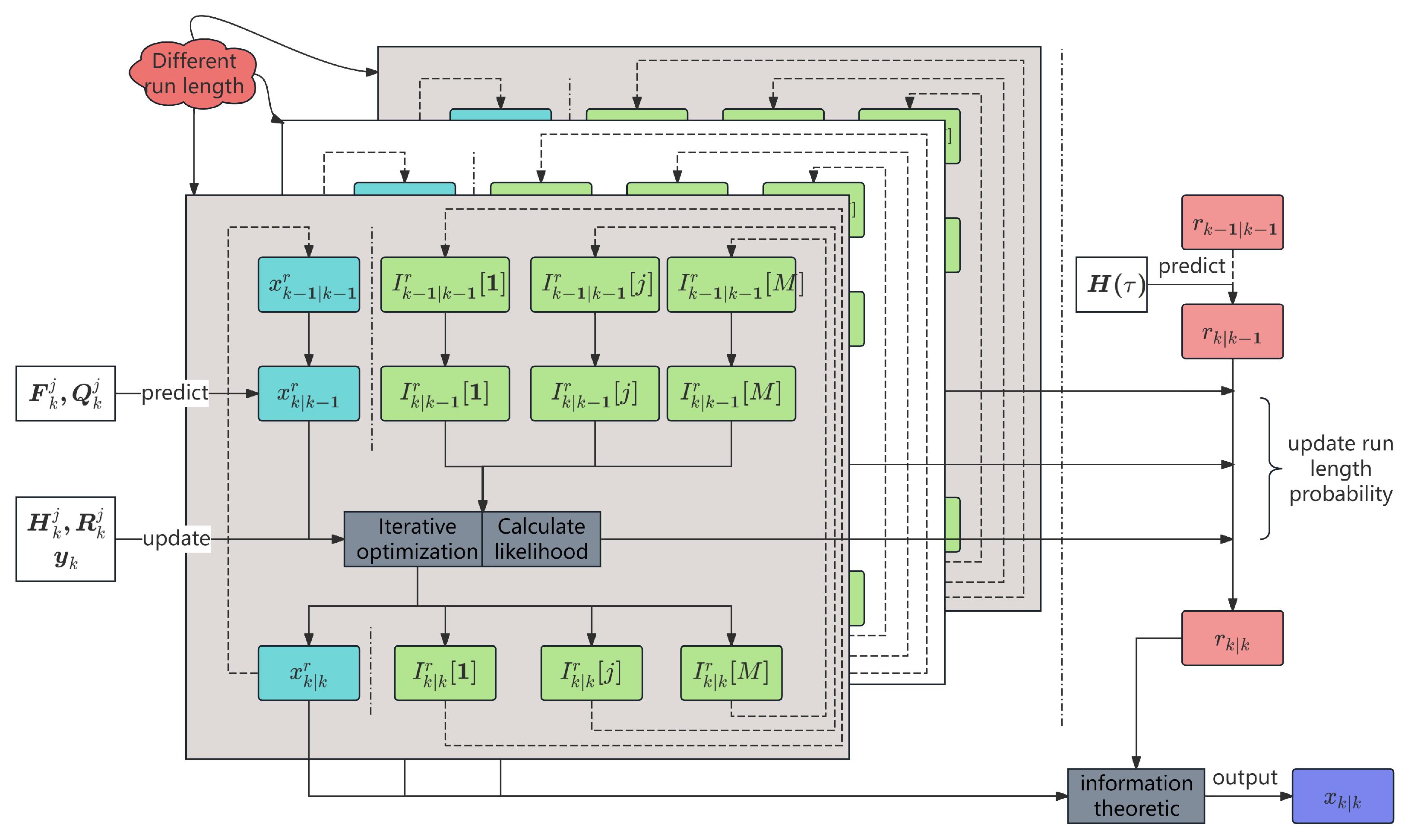
The proposed VBOCPDMS algorithm can be summarized in Algorithm 1.

Algorithm 1 VBOCPDMS: variational Bayesian online change-point detection with model selection.

Require:  Measurement ${\mathit{y}}_k$, approximated posterior pdfs $q\left({\mathit{x}}_{k-1}^r\right)$, $q\left({\mathit{I}}_{k-1}^r\right)$, $p\left({\mathit{r}}_{k-1}\right)$ at last time, iterations $N_{max}$, model domain $\mathcal{M}$, detection threshold ${\delta }_r$, penalty function $H\left(\tau \right)$; Ensure:  Approximated posterior pdfs $q\left({\mathit{x}}_{k-1}^r\right)$, $q\left({\mathit{I}}_{k-1}^r\right)$, $q\left({\mathit{x}}_k\right)$, $q\left({\mathit{I}}_k\right)$ and $p\left({\mathit{r}}_{k-1}\right)$ at current time;   1: Time prediction:   2: Calculate prior pdf $p\left({\mathit{x}}_k^r\right|y_{1:k-1})$ via (6)   3: Calculate prior pdf $p\left({\mathit{I}}_k^r\right|y_{1:k-1})$ via (13)   4: Calculate prior pdf $p\left({\mathit{r}}_k\right|y_{1:k-1})$ via (12)   5: Measurement update:   6: update run length parameters via (16)   7: Initialization:   8:     $q^{\left(0\right)}\left({\mathit{x}}_k^r\right)=p\left({\mathit{x}}_k^r\right|y_{1:k-1})$, $q^{\left(0\right)}\left({\mathit{I}}_k^r\right)=p\left({\mathit{I}}_k^r\right|y_{1:k-1})$;   9: for all$n=1:N_{max }$do 10:   update posterior $q\left({\mathit{x}}_{k-1}^r\right)$: update variational parameters via (37) and (38) 11:   update posterior $q\left({\mathit{I}}_{k-1}^r\right)$: update variational parameters via (41) 12: end for 13: Hybrid estimation: 14: Calculate state estimation $\widehat{{\mathit{x}}_k}$ and corresponding covariance $\widehat{{\mathit{P}}_k}$ via (49) and (50); 15: New run length initialization: 16: Calculate the likelihood $p\left({\mathit{y}}_k\right|{\mathit{y}}_{1:k-1})$ and select the ${\widehat{\mathit{\mu }}}_0^{*}$ via (15) 17: Change point detection: 18: Calculate the MAP estimate $r_k^{*}$ of ${\mathit{r}}_k$ via (27)

Remark 2. 

The computational complexity of the proposed algorithm primarily arises from two factors: (1) the increasing number of run-lengths over time, and (2) the iterative optimization required for variational inference. To address the first issue, we adopted the pruning strategy proposed in [29], which effectively controls the growth of the run-lengths. In theory, pruning the number of run-lengths may lead to a decrease in algorithm performance. However, it is important to note that the performance improvement gained from increasing the number of run-lengths is also limited. Experimental analysis shows that when the number of run-lengths is kept around 15, the algorithm strikes a good balance between computational load and filtering accuracy.

To address the second issue, we propose two parameter settings to reduce the number of iterations. The first is the most intuitive approach—setting the maximum iteration $I_{max}<5$. Since the average number of iterations in the experiments is around 5, reducing $I_{max}$ naturally reduces the computational load, and even with $I_{max}=1$, the algorithm still outperforms the comparison algorithms in terms of accuracy. Alternatively, we can set the $2a$ value in the reinitialization model weights to be close to 1. This approach brings the initial weights closer to the true weights during maneuvers, resulting in an average iteration count of around 2, with minimal loss in filtering accuracy. Therefore, this is the most recommended method for reducing computational burden in engineering applications.

These conclusions are supported by the experiments in Section 4.1.5. Additionally, since the state filtering computations for different run-lengths are independent, parallel computing can be employed to further reduce runtime when hardware resources are sufficient.

4. Experimental Evaluation

We evaluate the proposed VBOCPDMS algorithm against existing methods using six aerial maneuvering simulations and two real scenarios. Performance was measured by tracking accuracy and maneuver detection capability.

4.1. Simulation Scenarios

4.1.1. Scenario Setup

In this study, we employ the following six representative simulation scenarios for high-speed, highly maneuvering aerial targets as proposed in [33]. In all scenarios, the total number of steps is set to 186 with a measurement sampling period of T = 1 s. The measurement noise is defined as $\mathbf{R}=\mathrm{diag}({10}^4,{10}^4)$. The target trajectories for the six simulation scenarios are shown in Figure 2, and the details are described as follows.

S1 (shown in Figure 2a): The target is a large aircraft. During the intervals $k\in [60,79)$ and $k\in [111,130)$, the aircraft executes turning maneuvers with accelerations of $2\mathrm{g}$ (with $\mathrm{g}$ representing gravitational acceleration) and $3\mathrm{g}$, respectively. At all other times, the target maintains uniform linear motion. The change-point instants for this scenario are $[60,79,111,130]$.

S2 (shown in Figure 2b): The target is a small, agile aircraft. During the intervals $k\in [31,54)$ and $k\in [101,115)$, the aircraft performs a ${90}^{\circ }$ turn with an acceleration of $2.5\mathrm{g}$ and a turn with an acceleration of $4\mathrm{g}$, respectively. In the interval $k\in [54,101)$, the target gradually decelerates, while it maintains a constant speed during the remaining periods. The change-point instants for this scenario are $[31,54,101,115]$.

S3 (shown in Figure 2c): The target is a high-speed, medium-sized bomber. During the intervals $k\in [31,40)$ and $k\in [75,91)$, the bomber performs a ${45}^{\circ }$ turn with an acceleration of $4\mathrm{g}$ and a ${90}^{\circ }$ turn with an acceleration of $4\mathrm{g}$, respectively. Between $k\in [91,115)$, the target continues turning while gradually decelerating; during all other periods, it maintains uniform linear motion. The change-point instants for this scenario are $[31,40,75,91,115]$.

S4 (shown in Figure 2d): The target is a high-speed, medium-sized bomber. During the intervals $k\in [31,40)$ and $k\in [72,91)$, the aircraft executes a ${45}^{\circ }$ turn with an acceleration of $4\mathrm{g}$ and a turn with an acceleration of $6\mathrm{g}$, respectively. At other times, the target moves at a constant speed in the horizontal plane. The change-point instants for this scenario are $[31,40,72,82,91,136]$.

S5 (shown in Figure 2e): The target is a fighter aircraft whose trajectory comprises three constant turning maneuvers, accompanied by significant acceleration throughout the flight. Specifically, the turning intervals are $k\in [30,40)$, $k\in [60,72)$, and $k\in [118,128)$, with corresponding turning accelerations of $5\mathrm{g}$, $7\mathrm{g}$, and $6\mathrm{g}$, respectively. The change-point instants for this scenario are $[30,40,60,72,118,130,143,163]$.

S6 (shown in Figure 2f): The target is a fighter aircraft with a trajectory that includes four turning maneuvers. After the second turn, the aircraft reduces its altitude and speed before initiating the third turn; following the third turn, it rapidly accelerates to enter the fourth turn. The turning intervals are $k\in [31,45)$, $k\in [70,87)$, $k\in [116,132)$, and $k\in [151,160)$, with corresponding turning accelerations of $7\mathrm{g}$, $6\mathrm{g}$, $6\mathrm{g}$, and $7\mathrm{g}$, respectively. The change-point instants for this scenario are $[31,45,70,87,116,132,151,160]$.

4.1.2. Algorithm Parameter Settings

Considering that the models differ only in the process noise covariance matrix and should cover various motion modes ranging from nearly constant velocity to highly maneuvering behavior, the state dimension is set as $n_x=4$, and the state transition model is based on uniform linear motion. The corresponding model parameters are as follows:

$$\begin{array}{c}\hfill {\mathit{F}}_k={\mathit{I}}_2\otimes \left[\begin{array}{cc}1& T\\ 0& 1\end{array}\right]{\mathit{Q}}_k={\sigma }_q^2\times {\mathit{I}}_2\otimes \left[\begin{array}{cc}{T}^4/4& T^3/2\\ T^3/2& T^2\end{array}\right]\end{array}$$

(51)

Assuming a linear measurement model, the measurement transformation matrix ${\mathit{H}}_k$ and measurement noise matrix ${\mathit{R}}_k$ are given by:

$$\begin{array}{c}\hfill {\mathit{H}}_k=\left[\begin{array}{cccc}1& 0& 0& 0\\ 0& 0& 1& 0\end{array}\right]{\mathit{R}}_k={10}^4\times \left[\begin{array}{cc}1& 0\\ 0& 1\end{array}\right]\end{array}$$

(52)

Thus, for the relatively weak maneuvering scenarios (S1 and S2), the set of process noise models is defined as ${\sigma }_q\in \{10,20,40\}/2$, while for the strongly maneuvering scenarios (S3–S6), the process noise models are set as ${\sigma }_q\in \{10,20,40\}$.

• IMM [7]: This is the standard interacting multiple model filter, whose model weights are initialized using $[1/3,1/3,1/3]$.
• IEE [24]: This is an information theoretic IMM, whose model weights are initialized using $[1/3,1/3,1/3]$.
• IT-IMM [32]: This is a multi-model filter based on VB, whose model weights are initialized using $[1/3,1/3,1/3]$.
• VBOCPDMS: The filter mode weights are initialized using $[1/3,1/3,1/3]$. When a change point is assumed to exist, there are three possible choices for reinitializing the weights: $I_0=[0.8,0.1,0.1]$, $I_1=[0.1,0.8,0.1]$, and $I_2=[0.1,0.1,0.8]$, which respectively indicate that the maneuver at the change point is biased toward a specific mode. The maximum number of iterations is $I_{max}=50$, the maximum number of retained run lengths is set to $N_{max}=10$, and the penalty function is defined as $H\left(\tau \right)=15/186$.

For IMM, IT-IMM and IEE filters, the mode transition probability matrix ${\mathit{P}}_m$ is defined as:

$$\begin{array}{c}\hfill {\mathit{P}}_m=\left[\begin{array}{ccc}0.9& 0.05& 0.05\\ 0.05& 0.9& 0.05\\ 0.05& 0.05& 0.9\end{array}\right]\end{array}$$

(53)

For the proposed VBOCPDMS algorithm, the iterative process is terminated when the difference between successive state estimates is below a given threshold (e.g., when $\left|\right|{\widehat{x}}_k^{(n+1)}-{\widehat{x}}_k^{\left(n\right)}\left|\right|<1e-6$) or when the maximum number of iterations $I_{max}=50$ is reached. In addition, we conduct 100 Monte Carlo runs for each simulation scenario.

4.1.3. Performance Evaluation Metrics

The tracking performance of the target position is evaluated using the root mean square error (RMSE) and the average root mean square error (ARMSE) for the target position. The RMSE and ARMSE are calculated as follows. In this paper, these metrics are adopted to assess tracking accuracy:

$$\begin{array}{cc}\hfill & {\mathrm{RMSE}}_{\mathrm{pos}}\triangleq \sqrt{{\displaystyle \frac{1}{N_t}}\mathbf{\sum }_{N_t}\left[{(p_k^x-p_{k,t}^x)}^2+{(p_k^y-p_{k,t}^y)}^2\right]}\hfill \end{array}$$

(54a)

$$\begin{array}{cc}\hfill & {\mathrm{ARMSE}}_{\mathrm{pos}}\triangleq {\displaystyle \frac{1}{N_s}}\mathbf{\sum }_{N_s}{\mathrm{RMSE}}_{\mathrm{pos}}\hfill \end{array}$$

(54b)

Here, $N_s$ denotes the number of Monte Carlo simulation runs, $N_t$ represents the total number of simulation steps, $p_k^x$ and $p_{k,t}^x$ indicate the estimated and true positions in the x-direction at time k, respectively, while $p_k^y$ and $p_{k,t}^y$ denote the estimated and true positions in the y-direction.

For evaluating the change-point detection capability of the proposed VBOCPDMS algorithm, an improved F1-score is used to quantify detection accuracy. This metric is selected because the exact positions of change-points in real time-series data may be subject to randomness (e.g., process noise, measurement noise), and experts seldom agree on the precise locations of change-points. To address this issue, following the approach in [28], change-point detection is formulated as a classification problem between “change-point” and “non-change-point”. The F1-score is then computed as:

$$\begin{array}{c}\hfill F_1={\displaystyle \frac{2\mathcal{P}\mathcal{R}}{\mathcal{P}+\mathcal{R}}}\end{array}$$

(55)

where $\mathcal{P}$ denotes precision (the ratio of correctly detected change-points to the total number of detected change-points), and $\mathcal{R}$ denotes recall (the ratio of correctly detected change-points to the total number of true change-points).

As mentioned earlier, the calculation of the F1-score requires a clear definition of correct change-point detection. Specifically, if the algorithm detects a change-point within a tolerance range $\mathcal{E}\ge 0$ of a true change-point, then that detection is considered correct. Furthermore, to avoid double counting, only one detection within the tolerance range $\mathcal{E}$ around a true change-point is counted as a true positive. Formally, let C denote the set of change-points detected by the algorithm, T the set of true change-points, and $\mathcal{D}(T,C)$ the set of true change-points that have been detected. For each $\gamma \in \mathcal{D}(T,C)$, there exists a $c\in C$ such that $\left|\gamma -c\right|\le \mathcal{E}$, and each true change-point $\gamma$ is associated with only one such c. Based on this definition, the precision $\mathcal{P}$ and recall $\mathcal{R}$ are computed as:

$$\begin{array}{c}\hfill \mathcal{P}={\displaystyle \frac{\left|\mathcal{D}\right(T,C\left)\right|}{\left|C\right|}}\mathcal{R}={\displaystyle \frac{\left|\mathcal{D}\right(T,C\left)\right|}{\left|T\right|}}\end{array}$$

(56)

4.1.4. Results

Figure 3 presents the ARMSE curves of the target position under different scenarios for four filtering algorithms. Gray dashed lines indicate the change points of the target’s acceleration, i.e., the onset of maneuvers. Different filtering algorithms are represented by distinct curve markers: the IMM algorithm is depicted with blue square markers, the IEE algorithm with orange cross markers, the IT-IMM algorithm is depicted with green circle markers, and the proposed VBOCPDMS algorithm with red asterisk markers. Subfigures (a) to (f) correspond to simulation scenarios S1 through S6, respectively.

All algorithms perform similarly in non-maneuvering segments due to their different motion models and optimal mixed estimation via probabilistic weighting. The VBOCPDMS algorithm, however, outperforms IMM, IEE, and IT-IMM, benefiting from variational iterative optimization for better handling of non-maneuvering models.

During the maneuver process, the RMSE of IMM, IEE and IT-IMM all increased significantly, especially after a change point. Among them, the increase of IEE was the largest, followed by that of IT-IMM, and the increase of IMM was relatively small. In contrast, the VBOCPDMS algorithm’s RMSE also rises but declines faster than the baseline algorithms. IMM shows a trade-off, achieving better accuracy in non-maneuvering scenarios at the cost of poorer accuracy during maneuvers. VBOCPDMS achieves good estimation accuracy during maneuvers by adaptively adjusting prior model weights based on run length and switching models promptly. In contrast, IMM, IEE, and IT-IMM use fixed prior weights and transition matrices, causing delays in model switching and competition between models, which degrades performance. VBOCPDMS speeds up parameter estimation by using hard-decision initialization to reduce secondary model weights during maneuvers.

Table 1. Average position RMSE (m) of different algorithms in scenarios S1–S6.

Algorithm	S1	S2	S3	S4	S5	S6
IEE	95.587	98.596	94.848	94.196	105.310	108.680
IMM	86.492	87.477	90.105	89.937	96.586	98.331
IT-IMM	85.052	86.078	87.513	87.297	95.88	97.799
VBOCPDMS	81.530	80.024	86.096	85.128	92.754	94.474

shows that the VBOCPDMS filtering algorithm outperforms IMM, IEE, and IT-IMM in filtering accuracy across six simulation scenarios, with average RMSE rankings of VBOCPDMS < IT-IMM < IMM < IEE. VBOCPDMS effectively detects target maneuvering pattern changes through online change-point detection for timely responses. It uses run-length probability weighting for maximum entropy in state estimation, demonstrating superior tracking accuracy in all scenarios.

Figure 4 illustrates the true and estimated trajectories across six simulation scenarios. Our proposed algorithm (red) closely follows the true trajectory (black) during target maneuvers, unlike the IEE algorithm (orange), which deviates significantly. This supports our analysis showing the proposed method’s superior accuracy, especially during abrupt maneuvers where traditional algorithms falter.

Table 2. Average runtime (s) of different algorithms in the simulation scenarios.

Algorithms	S1	S2	S3	S4	S5	S6
IEE	0.0093	0.0091	0.0081	0.0092	0.0077	0.0078
IMM	0.0151	0.0142	0.0132	0.0135	0.0123	0.0124
IT-IMM	0.0227	0.0213	0.0203	0.0215	0.0184	0.0189
VBOCPDMS	0.7830	0.5769	0.5918	0.6351	0.5989	0.6181

analyzes the computational costs of various algorithms. The IEE algorithm has the highest efficiency and the shortest running time, followed by the IMM algorithm. The running time of the IT-IMM algorithm is relatively slightly longer. Conversely, the proposed VBOCPDMS algorithm is slower due to iterative computation for estimating posterior states and weights. Meanwhile, it incorporates maneuver detection, requiring an extra discrete variable estimated at each time step, growing with time.

Table 3. Average number of iterations of the VBOCPDMS algorithm in the simulation scenarios.

Algorithms	S1	S2	S3	S4	S5	S6
VBOCPDMS	4.3116	4.3032	4.9460	4.8916	5.1058	5.1662

shows the average iteration count across scenarios of VBOCPDMS, all notably below the maximum limit $I_{max}=50$, indicating good convergence.

To evaluate the effectiveness and accuracy of the VBOCPDMS algorithm in change point detection,

Table 4. F1-scores of the VBOCPDMS algorithm.

Threshold	S1	S2	S3	S4	S5	S6
$\mathcal{E}=\mathbf{5}$	0.3468	0.4186	0.4230	0.5799	0.6214	0.6399
$\mathcal{E}=\mathbf{10}$	0.6272	0.6552	0.7389	0.8403	0.8484	0.8961

presents the F1-scores under different scenarios. By analyzing these data, it can be observed that in scenarios with weak target maneuverability (such as S1), the algorithm’s F1-score is relatively low. In contrast, in scenarios with stronger maneuverability or higher maneuvering frequency (such as S6), the F1-score improves significantly. This suggests that the strength and frequency of target maneuvers have a notable impact on the algorithm’s change point detection performance—the stronger the maneuverability, the better the detection effect.

Furthermore, it is worth noting that when a larger tolerance range $\mathcal{E}$ is selected, the algorithm’s F1-score exhibits an obvious upward trend, reflecting that change point detection has a certain degree of latency. However, this does not indicate that the proposed algorithm struggles with handling target maneuvers. In fact, the VBOCPDMS algorithm inherently possesses the ability to identify maneuver parameters (i.e., estimate run length probability). Under the variational Bayesian joint optimization framework, change point detection and maneuver parameter identification are inherently coupled. If the algorithm can effectively respond to the ongoing maneuvering change point through parameter estimation, it can effectively alleviate the problem of model mismatch caused by model switching delay. Therefore, the accuracy of change point detection is no longer an absolute evaluation criterion, but depends on the actual ability of the algorithm to effectively deal with maneuvering change points.

4.1.5. Robustness Analysis

To verify the robustness of the proposed algorithm under various parameter settings and to further elucidate the roles of these parameters during the filtering process, a series of controlled experiments were conducted in this subsection. Considering that scenarios S1 and S2 involve relatively weak target maneuvers, and that demonstrating robustness under strong maneuvering conditions is more convincing, we selected simulation scenarios S3 through S6 for the robustness analysis. In each scenario, the focus was placed on the variation of a single algorithm parameter.

Table 5. The average position RMSE (m) of $H\left(\tau \right)$ with different values in scenarios S3 to S6.

$\mathit{H}\left(\mathit{\tau }\right)$	S3	S4	S5	S6
5/186	85.676	85.768	94.649	97.068
10/186	85.034	85.110	93.950	96.183
15/186	86.096	85.128	92.754	94.474
20/186	85.240	85.232	93.851	95.478

analyzes the impact of varying parameter $H\left(\tau \right)$ on the performance of the VBOCPDMS algorithm. In scenarios S3 and S4, the ARMSE is minimized when the parameter $H\left(\tau \right)$ is set to 10, whereas in scenarios S5 and S6, the minimum ARMSE occurs when the parameter $H\left(\tau \right)$ is set to 15. This is because the parameter $H\left(\tau \right)$ essentially reflects the maneuvering frequency of the target. Targets in scenarios S3 and S4 exhibit relatively lower maneuvering frequencies, corresponding to a parameter value of 10, while targets in scenarios S5 and S6 have higher maneuvering frequencies, corresponding to a parameter value of 15. A properly selected parameter $H\left(\tau \right)$ can effectively capture the target’s maneuvering behavior, thereby achieving the best filtering performance. When the parameter selection is not perfectly aligned with the actual maneuvering frequency, the filtering performance slightly degrades; however, it still outperforms the baseline algorithms overall.

Table 6. The average position RMSE (m) of maximum iterations $I_{\mathit{m}\mathit{a}\mathit{x}}$ with different values in scenarios S3 to S6.

${\mathit{I}}_{\mathit{max}}$	S3	S4	S5	S6
1	85.273	85.390	94.351	96.317
2	85.012	85.115	93.917	95.812
10	84.953	85.014	93.768	95.646
50	85.005	85.128	92.754	94.474

analyzes the impact of varying parameter $I_{\mathit{m}\mathit{a}\mathit{x}}$ on the performance of the VBOCPDMS algorithm. Given that the average number of iterations required for convergence is approximately five, it can be observed that the minimum ARMSE across all four scenarios is achieved when the maximum allowable iterations are set to either 10 or 50. Moreover, once the number of iterations exceeds five, the filtering performance exhibits negligible further changes, indicating that convergence has been effectively achieved. It is particularly noteworthy that even when the number of iterations is limited to one or two, the proposed algorithm still outperforms the baseline methods. This property provides a valuable means to balance filtering accuracy and computational efficiency in practical engineering applications.

Table 7. The average position RMSE (m) of reinitialization model weights with different values in scenarios S3 to S6.

Weights	S3	S4	S5	S6	Iterations
$\mathbf{2}\mathit{a}$ = 1/3	90.963	90.033	94.961	95.587	6–7
$\mathbf{2}\mathit{a}$ = 0.7	86.152	85.134	92.762	94.495	5.2–5.7
$\mathbf{2}\mathit{a}$ = 0.8	86.096	85.128	92.754	94.474	4.8–5.2
$\mathbf{2}\mathit{a}$ = 0.9	86.130	85.134	92.742	94.462	4.2–4.5
$\mathbf{2}\mathit{a}$ = 1	86.028	85.167	92.757	94.468	1.8–2.2

analyzes the impact of varying reinitialization model weights on the performance of the VBOCPDMS algorithm. In the “weights” column of the table, the listed values correspond to $2a$, leading to the reinitialization model weights defined as $I_0=[2a,0.5-a,0.5-a]$, $I_1=[0.5-a,2a,0.5-a]$, and $I_2=[0.5-a,0.5-a,2a]$. It can be observed that when $2a=1/3$, corresponding to an equal distribution of initialization weights, the filtering performance is significantly degraded. In this case, the initialization weight selection mechanism effectively becomes inactive, resulting in uniformly distributed initial weights. As the initialization weights become more biased toward their respective models, the filtering performance improves. Moreover, as $2a$ approaches 1, the filtering accuracy remains consistently high, while the average number of iterations decreases from approximately seven to about two. This characteristic can be exploited in practical engineering applications to substantially reduce computational burden.

Table 8. The average position RMSE (m) of pruning threshold $N_{\mathit{m}\mathit{a}\mathit{x}}$ with different values in scenarios S3 to S6.

${\mathit{N}}_{\mathit{max}}$	S3	S4	S5	S6
5	100.040	99.891	102.550	103.330
10	86.096	85.128	92.754	94.474
15	85.885	85.018	92.424	94.281

analyzes the impact of varying pruning threshold $N_{\mathit{m}\mathit{a}\mathit{x}}$ on the performance of the VBOCPDMS algorithm. When the pruning threshold $N_{\mathit{max}}=5$, the filtering performance of the VBOCPDMS algorithm is inferior to that of the baseline methods. However, as the pruning threshold increases, the filtering performance gradually improves and eventually converges. This observation indicates that the number of retained run-lengths should be greater than 10 to achieve satisfactory performance. Further increasing the number of run-lengths yields only marginal performance gains while significantly increasing the computational burden, which is therefore not recommended.

4.2. Real Scenarios

In this section, we further evaluate the estimation performance of the proposed algorithm in two sets of real maneuvering target tracking scenarios by using the two-dimensional radar dataset.

4.2.1. Scenario Setup

The targets are detected and tracked using radar. The motion patterns of the two targets are detailed as follows:

R1 (shown in Figure 5a): This target performs a composite maneuver consisting of six segments: uniform motion, left turn, uniform motion, right turn, uniform acceleration, and a figure-eight circling pattern. The true change points in its motion occur at frames [13, 23, 34, 66, 73, 81, 116, 102]. The radar sampling interval is $T=10\mathrm{s}$, and the sequence comprises a total of 121 frames.

R2 (shown in Figure 5b): It also follows a six-segment composite maneuver: uniform motion, left turn, uniform motion, right turn, uniform motion, and an O-shaped circling pattern. The actual maneuver transition points are located at frames [13, 34, 65, 80, 100]. The radar sampling interval is $T=10 \mathrm{s}$, with a total of 105 frames.

4.2.2. Algorithm Parameter Settings and Performance Evaluation Metrics

Real scenarios use the same matrix forms as simulations. In R1, the process noise model set is ${\sigma }_q\in \{20,35,50\}$ and the change-point detection probability for VBOCPDMS is $49/\mathrm{NStep}$. In R2, the process noise model set is ${\sigma }_q\in \{5,15,30\}$ and the change-point detection probability is $15/\mathrm{NStep}$.

The reinitialization model weights are given by $I_0=[0.01,0.495,0.495]$, $I_1=[0.1,0.8,0.1]$ and $I_2=[0.1,0.1,0.8]$; the maximum number of retained run lengths is set to $N_{max}=15$ for the two real scenarios. Other parameters remain identical to those in the simulation scenarios, and the performance evaluation metrics are the same.

4.2.3. Results

Figure 6 shows the RMSE curves for target position estimation across different algorithms in scenarios R1 and R2.

Table 9. RMSE (m) of different algorithms in the real scenarios.

Scenario	IT-IMM	IMM	IEE	VBOCPDMS
R1	546.43	546.05	545.79	540.46
R2	381.27	367.04	320.63	313.91

provides the ARMSE for these algorithms in both scenarios, highlighting VBOCPDMS’s superior filtering performance. In scenario R2, RMSE curves are similar across algorithms during non-maneuvering or weakly maneuvering states, but VBOCPDMS stands out significantly once the target starts maneuvering.

Table 10. The segmented RMSE (m) of different algorithms in real scenario R1.

Section	IT-IMM	IMM	IEE	VBOCPDMS
$[0,\mathrm{G}1)$	356.69	358.51	360.45	366.75
$[\mathrm{G}1,\mathrm{G}2)$	178.2	178.67	179.2	185.59
$[\mathrm{G}2,\mathrm{G}3)$	162.5	162.48	162.37	161.9
$[\mathrm{G}3,\mathrm{G}4)$	230.7	230.65	230.6	230.07
$[\mathrm{G}4,\mathrm{G}5)$	486.48	485.61	484.84	471.99
$[\mathrm{G}5,\mathrm{G}6)$	1220.2	1217.6	1218.2	1200.4
$[\mathrm{G}6,\mathrm{G}7)$	921.3	921.75	921.48	923.42
$[\mathrm{G}7,\mathrm{G}8)$	1038.3	1036.6	1034.6	1012.3
$[\mathrm{G}8,121]$	611.03	605.3	603.98	566.39

and

Table 11. The segmented RMSE (m) of different algorithms in real scenario R2.

Section	IT-IMM	IMM	IEE	VBOCPDMS
$[0,\mathrm{H}1)$	366.69	361.53	343.72	315.16
$[\mathrm{H}1,\mathrm{H}2)$	283.49	260.54	197.05	121.29
$[\mathrm{H}2,\mathrm{H}3)$	288.23	284.06	283.99	277.64
$[\mathrm{H}3,\mathrm{H}4]$	488.35	467.52	467.13	358.69
$[\mathrm{H}4,\mathrm{H}5]$	482.9	457.33	496.21	450.86
$[\mathrm{H}5,105]$	784.03	759.62	850.21	784.55

detail the RMSE values across different filtering algorithms under various conditions. When the target moves uniformly or with slight turns, all methods perform similarly. However, as turns or acceleration increase, performance decreases. The VBOCPDMS algorithm remains more robust in handling maneuvers, surpassing both the IT-IMM, IMM, and IEE algorithms overall. This is because the IMM algorithm depends on the model transition probability matrix for model switching, which can cause delays and errors if the matrix is inaccurate during strong target maneuvers. Conversely, the VBOCPDMS algorithm uses Bayesian online change point detection for model selection without relying on this matrix, allowing for timely reinitialization of model weights and target states. This adaptability enhances the accuracy and stability of the VBOCPDMS algorithm in managing complex maneuvers.

Table 12. Runtime (s) of different algorithms in the real scenarios.

Scenarios	IT-IMM	IMM	IEE	VBOCPDMS
R1	0.0109	0.0103	0.0043	0.4570
R2	0.0085	0.0160	0.0063	0.4099

shows the computational cost comparison for different algorithms in real scenarios, supporting the previous simulation analysis and confirming the cost characteristics of the VBOCPDMS algorithm. The higher cost is mainly due to online change-point detection and variational iterative optimization.

With an error range of $\mathcal{E}=5$, the F1-scores of VBOCPDMS in scenarios R1 and R2 were $0.4000$ and $0.2857$. Bayesian online change point detection is a soft decision-making method based on manually defined rules. Evaluating it with a single metric is insufficient; thus, the filtering results are crucial, with the F1-score as a secondary criterion.

5. Conclusions

This paper presents a novel maneuvering target tracking method, VBOCPDMS, which integrates variational Bayesian inference and run-length modeling to capture maneuver change points in real time. Within the variational framework, the approximate posterior distributions of the motion state, model weights, and run-length are jointly estimated. The introduction of the run-length variable not only enables accurate detection of change points but also facilitates the adaptive reconfiguration of the algorithm’s parameters during abrupt target maneuvers. Unlike traditional IMM algorithms, which assume a first-order Markov process for model transitions, the proposed method explicitly tracks the run-length, modeling the system evolution in a non-Markovian manner. This design allows VBOCPDMS to retain a longer memory of past system dynamics, which is crucial for accurately capturing sudden maneuver onsets and maintaining robust tracking performance under highly dynamic conditions. Extensive experiments were conducted across six simulation scenarios and two real-world scenarios. The results demonstrate that VBOCPDMS consistently outperforms baseline methods such as IMM, IT-IMM, and IEE in terms of RMSE and maneuver-adaptive responsiveness, especially in cases involving high accelerations and abrupt turns. Furthermore, the proposed method exhibits strong robustness to model parameter uncertainties, highlighting its potential for real-time applications, such as radar surveillance. In future work, further research will be devoted to extending the VBOCPDMS framework to accommodate high-dimensional state spaces and multi-target tracking scenarios.

References

1. Li, X.R.; Jilkov, V.P. Survey of maneuvering target tracking. Part I: Dynamic models. IEEE Trans. Aerosp. Electron. Syst. 2003, 39, 1333–1363. [Google Scholar]
2. Li, X.R.; Jilkov, V.P. Survey of maneuvering target tracking. Part V: Multiple-model methods. IEEE Trans. Aerosp. Electron. Syst. 2005, 41, 1255–1321. [Google Scholar]
3. Punithakumar, K.; Kirubarajan, T.; Sinha, A. Multiple-model probability hypothesis density filter for tracking maneuvering targets. IEEE Trans. Aerosp. Electron. Syst. 2008, 44, 87–98. [Google Scholar] [CrossRef]
4. Blackman, S.S. Multiple hypothesis tracking for multiple target tracking. IEEE Aerosp. Electron. Syst. Mag. 2004, 19, 5–18. [Google Scholar] [CrossRef]
5. Guo, Y.; Huang, B. Moving horizon estimation for switching nonlinear systems. Automatica 2013, 49, 3270–3281. [Google Scholar] [CrossRef]
6. Watanabe, K.; Tzafestas, S.G. Generalized pseudo-Bayes estimation and detection for abruptly changing systems. J. Intell. Robot. Syst. 1993, 7, 95–112. [Google Scholar] [CrossRef]
7. Blom, H.A.P.; Bar-Shalom, Y. The interacting multiple model algorithm for systems with Markovian switching coefficients. IEEE Trans. Autom. Control 1988, 33, 780–783. [Google Scholar] [CrossRef]
8. Liu, W.; Zhang, H.; Wang, Z. A novel truncated approximation based algorithm for state estimation of discrete-time Markov jump linear systems. Signal Process. 2011, 91, 702–712. [Google Scholar] [CrossRef]
9. Pourbabaee, B.; Meskin, N.; Khorasani, K. Sensor fault detection, isolation, and identification using multiple-model-based hybrid Kalman filter for gas turbine engines. IEEE Trans. Control Syst. Technol. 2015, 24, 1184–1200. [Google Scholar] [CrossRef]
10. Qiu, J.; Xing, Z.; Zhu, C.; Lu, K.; He, J.; Sun, Y.; Yin, L. Centralized fusion based on interacting multiple model and adaptive Kalman filter for target tracking in underwater acoustic sensor networks. IEEE Access 2019, 7, 25948–25958. [Google Scholar] [CrossRef]
11. Youn, W.; Ko, N.Y.; Gadsden, S.A.; Myung, H. A novel multiple-model adaptive Kalman filter for an unknown measurement loss probability. IEEE Access 2020, 70, 1–11. [Google Scholar] [CrossRef]
12. Qu, H.; Pang, L.; Li, S. A novel interacting multiple model algorithm. Signal Process. 2009, 89, 2171–2177. [Google Scholar] [CrossRef]
13. Sheng, H.; Zhao, W.; Wang, J. Interacting multiple model tracking algorithm fusing input estimation and best linear unbiased estimation filter. IET Radar Sonar Navig. 2017, 11, 70–77. [Google Scholar] [CrossRef]
14. Xu, L.; Li, X.R.; Duan, Z. Hybrid grid multiple-model estimation with application to maneuvering target tracking. IEEE Trans. Aerosp. Electron. Syst. 2016, 52, 122–136. [Google Scholar] [CrossRef]
15. Arulampalam, M.S.; Maskell, S.; Gordon, N.; Clapp, T. A tutorial on particle filters for online nonlinear/non-Gaussian Bayesian tracking. IEEE Trans. Signal Process. 2002, 50, 174–188. [Google Scholar] [CrossRef]
16. Özkan, E.; Smídl, V.; Saha, S.; Lundquist, C.; Gustafsson, F. Marginalized adaptive particle filtering for nonlinear models with unknown time-varying noise parameters. Automatica 2013, 49, 1566–1575. [Google Scholar] [CrossRef]
17. Blei, D.M.; Kucukelbir, A.; McAuliffe, J.D. Variational inference: A review for statisticians. J. Am. Stat. Assoc. 2017, 112, 859–877. [Google Scholar] [CrossRef]
18. Särkkä, S.; Nummenmaa, A. Recursive noise adaptive Kalman filtering by variational Bayesian approximations. IEEE Trans. Autom. Control 2009, 54, 596–600. [Google Scholar] [CrossRef]
19. Mbalawata, I.S.; Särkkä, S.; Vihola, M.; Haario, H. Adaptive Metropolis algorithm using variational Bayesian adaptive Kalman filter. Comput. Stat. Data Anal. 2015, 83, 101–115. [Google Scholar] [CrossRef]
20. Dong, P.; Jing, Z.; Leung, H.; Shen, K. Variational Bayesian adaptive cubature information filter based on Wishart distribution. IEEE Trans. Autom. Control 2017, 62, 6051–6057. [Google Scholar] [CrossRef]
21. Huang, Y.; Zhang, Y.; Wu, Z.; Li, N.; Chambers, J. A Novel Adaptive Kalman Filter with Inaccurate Process and Measurement Noise Covariance Matrices. IEEE Trans. Autom. Control 2018, 63, 594–601. [Google Scholar] [CrossRef]
22. Huang, Y.; Zhang, Y.; Shi, P.; Chambers, J. Variational adaptive Kalman filter with Gaussian-inverse-Wishart mixture distribution. IEEE Trans. Autom. Control 2020, 66, 1786–1793. [Google Scholar] [CrossRef]
23. Zhang, J.; Wei, G.; Ding, D.; Ju, Y. Distributed Sequential State Estimation Over Binary Sensor Networks with Inaccurate Process Noise Covariance: A Variational Bayesian Framework. IEEE Trans. Signal Inf. Process. Netw. 2025, 11, 1–10. [Google Scholar] [CrossRef]
24. Ma, Y.; Zhao, S.; Huang, B. Multiple-model state estimation based on variational Bayesian inference. IEEE Trans. Autom. Control 2018, 64, 1679–1685. [Google Scholar] [CrossRef]
25. Lan, H.; Hu, J.; Wang, Z.; Cheng, Q. Variational Nonlinear Kalman Filtering with Unknown Process Noise Covariance. IEEE Trans. Aerosp. Electron. Syst. 2023, 59, 9177–9190. [Google Scholar] [CrossRef]
26. Lan, H.; Zhao, S.; Hu, J.; Wang, Z.; Fu, J. Joint State Estimation and Noise Identification Based on Variational Optimization. IEEE Trans. Autom. Control 2024, 1–16. [Google Scholar] [CrossRef]
27. Lan, H.; Zhao, S.; Mao, Y.; Wang, Z.; Cheng, Q.; Liu, Z. Noise Adaptive Kalman Filtering with Stochastic Natural Gradient Variational Inference. IEEE Trans. Aerosp. Electron. Syst. 2025, 1–17. [Google Scholar] [CrossRef]
28. Van den Burg, G.J.J.; Williams, C.K.I. An evaluation of change point detection algorithms. arXiv 2020, arXiv:2003.06222. [Google Scholar]
29. Adams, R.P.; MacKay, D.J. Bayesian online changepoint detection. arXiv 2007, arXiv:0710.3742. [Google Scholar]
30. Hou, X.; Zhao, S.; Hu, J.; Lan, H. Noise-Adaptive State Estimators with Change-Point Detection. Sensors 2024, 24, 4585. [Google Scholar] [CrossRef]
31. Zhang, C.; Bütepage, J.; Kjellström, H.; Mandt, S. Advances in variational inference. IEEE Trans. Pattern Anal. Mach. Intell. 2018, 41, 2008–2026. [Google Scholar] [CrossRef] [PubMed]
32. Li, W.; Jia, Y. An information theoretic approach to interacting multiple model estimation. IEEE Trans. Aerosp. Electron. Syst. 2015, 51, 1811–1825. [Google Scholar] [CrossRef]
33. Blair, W.D.; Watson, G.A.; Kirubarajan, T.; Bar-Shalom, Y. Benchmark for radar allocation and tracking in ECM. IEEE Trans. Aerosp. Electron. Syst. 1998, 34, 1097–1114. [Google Scholar] [CrossRef]
Figure 1. VBOCPDMS method framework diagram.
Electronics 14 01908 g001
Figure 2. The target trajectories for six simulation scenarios: (a) Simulation scenario S1. (b) Simulation scenario S2. (c) Simulation scenario S3. (d) Simulation scenario S4. (e) Simulation scenario S5. (f) Simulation scenario S6.
Electronics 14 01908 g002
Figure 3. The ARMSE curves of the target positions of different algorithms in six simulation scenarios: (a) ARMSE curves in S1. (b) ARMSE curves in S2. (c) ARMSE curves in S3. (d) ARMSE curves in S4. (e) ARMSE curves in S5. (f) ARMSE curves in S6.
Electronics 14 01908 g003
Figure 4. True trajectory vs. inferred trajectory of different algorithms in six simulation scenarios: (a) Trajectory in S1. (b) Trajectory in S2. (c) Trajectory in S3. (d) Trajectory in S4. (e) Trajectory in S5. (f) Trajectory in S6.
Electronics 14 01908 g004
Figure 5. Target trajectory of real scenarios: (a) Real scenario R1. (b) Real scenario R2.
Electronics 14 01908 g005
Figure 6. The RMSE curves of the target position in real scenarios: (a) RMSE curves in R1. (b) RMSE curves in R2.
Electronics 14 01908 g006