Synthesis of the Large-Scaled 64 × 64 Thinned Array Using the Branch and Bound Technique with Convex Optimization for Satellite Communication

Abstract

This paper presents the synthesis of a 64 × 64 thinned array, using the branch and bound technique with convex optimization and a low sidelobe level for satellite communication. The branch and bound technology decomposes optimization into several subproblems. The convex optimization transforms the optimized variable binary [0, 1] of the thinned array into a continuous variable, i.e., from 0 to 1. Based on the branch and bound technique with convex optimization, the fast and accurate convergence of the synthesis of large-scale thinned array was achieved, and 2400 elements were selected for a full 64 × 64 array with a sidelobe level that satisfies the system requirements. The proposed thinned array with 2400 elements was simulated via full-wave 3D simulation. A prototype of the proposed thinned array was fabricated and measured. The simulated and measured results verified the effectiveness of the branch and bound technique with convex optimization.

1. Introduction

Due to its capability for global seamless coverage, satellite communication has been extensively studied in recent years [1]. Since 2017, the 3rd Generation Partnership Project (3GPP) has been exploring the integration of satellite communication with ground cellular systems for air–space integration technology, proposing technical standards to support non-terrestrial networks (NTNs) [2,3]. To achieve optimal spatial coverage, the radiation pattern of the array antenna for satellite communication should meet specific requirements, such as having a high gain, a narrow 3 dB beamwidth, and low sidelobe levels [4,5].

The synthesis of the array pattern, which can direct the main lobe to the desired direction with appropriate beamwidth and low sidelobe levels in other directions, has been widely studied [6]. However, as the number of array elements increases, the feeding network with TR-modules of a large-scale array becomes very complex and expensive [7]. A thinned array, created by removing some elements from a periodic array, offers a promising solution for large-scale arrays by maintaining low sidelobe levels and simplifying the feeding network [8]. In the textbook [6], methods such as Schelkunoff polynomial, Fourier transform, Woodward–Lawson, Taylor, and back-projection are proposed to achieve the desired array radiation pattern. However, due to the complexity of the desired pattern, such as multiple beam directions and stringent sidelobe level requirements, these methods often fall short of achieving the desired results. Also, the adaptively thinned [8], deterministic binary sequences [9], probability density tapering [10], modified iterative Fourier technique [11,12], precoded subarray structures [13], and perturbational method [14] are also proposed to synthesis of the thinned array.

Additionally, the nonlinear optimization methods derived from biological behavior [15,16,17,18,19,20,21,22], such as differential evolution (DE) [16,17], particle swarm optimization (PSO) [18], simulated annealing (SA) [19], invasive weed optimization (IWO) [20], and genetic algorithms (GAs) [21,22], are suitable for solving the nonlinear problems of the synthesis of the thinned array. These algorithms usually iteratively reduce the gap (objective function) between the desired and current radiation patterns. However, with large array scales, nonlinear optimization methods can be time-consuming and may struggle to converge. Furthermore, the neural network method is also applied to achieve the synthesis of the thinned array [23,24]. To realize superior performance, extensive data should be provided to train the neural network.

To achieve the synthesis of the large-scale thinned array, branch and bound technology with convex optimization is proposed and studied in this paper. Branch and bound technology can decompose optimization into several subproblems. The convex optimization can transform the optimized variable binary [0, 1] of the thinned array into the continues variable, i.e., from 0 to 1. Ultimately, the synthesis of the 64 × 64 thinned array with the desired radiation pattern is achieved. The simulated and measured results of a thinned array are presented to verify the results.

2. Formulation and Algorithm

In this section, the design is discussed first. Then, mathematical modeling is carried out to represent the object. Finally, the branch and bound technique with convex optimization used to solve the problem is outlined.

• Problem Statement

The full array has 64 × 64 elements and is shown in Figure 1. The element spacings between each element is a half-wavelength at the center frequency. For the thinned array, only 2400 elements of the full array can be selected. Also, as shown in Figure 1b, every 2 × 2 element as a subarray is deployed for a single transceiver. The thinned array selection is based on each 2 × 2 element. For the array radiation pattern, in the φ = 0°, φ = 45°, φ = 90°, and φ = 135° cut planes, the array pattern in the sidelobe region ($h\left(\theta ,\phi \right)$) should satisfy the following requirements:

$$h(\theta ,\phi )\le \left\{\begin{array}{ll}-9-25\times {\log }_{10}\left(\theta \right)dBi,& 2^{°}\le \theta \le 7^{°}\hfill \\ -30dBi,& 7^{°}\le \theta \le {9.2}^{°}\\ -6-25\times {\log }_{10}\left(\theta \right)dBi,& {9.2}^{°}\le \theta \le 48\\ -36dBi,& {48}^{°}\le \theta \le {90}^{°}\end{array}\right..$$

(1)

Also, for the symmetric of the array radiation pattern, most of the subarrays should line in the circle.

B.

Mathematical Modeling

A 2 × 2 subarray was designed for the full 64 × 64 array, where the sidelobe constraints are $h\left(\theta ,\phi \right)$. The binary integer matrix $\mathbf{B}\in {\mathrm{R}}^{32\times 32}$ was defined as the optimization variable. Here $B_{ij}=1$ means that 2 × 2 subarray was placed and $B_{ij}=0$ means that 2 × 2 subarray was not placed at one of the four positions $\left(2\mathrm{i}-\mathrm{1,2}\mathrm{j}-1\right),\left(2i-\mathrm{1,2}j\right)$, or $\left(2i,2j-1\right)$. Therefore, the selection matrix $\mathit{B}⨂l_{2\times 2}$ was achieved for the full array, where $⨂$ denotes the Kronecker product and $l_{2\times 2}$ denotes the 2 × 2 matrices.

Based on the construction, the constraints were transformed into a mathematical problem. Meanwhile, to ensure that most subarrays lie within the circle, the subarrays outside the circle were inactive, i.e., $B_{ij}=0,\left(i,j\right)\in \mathsf{\Phi }$, where $\mathsf{\Phi }$ denotes the set of indices for the subarrays outside the circle.

For the full 64 × 64 array, θ and φ denote the azimuth and elevation angle, and the response of the (m,n)th array element is ${a_{m,n}\left(\theta ,\phi \right)=e}^{j\left(\left(m-1\right)\pi cos\left(\phi \right)sin\left(\theta \right)+\left(n-1\right)\pi sin\left(\phi \right)sin\left(\theta \right)\right)}$. Therefore, given the distribution of the array, the array radiation pattern $f\left(\theta ,\phi \right)$ can be obtained as

$$\begin{array}{l}f\left(\theta ,\phi \right)={\displaystyle \sum _{m=1}^{64}{\displaystyle \sum _{n=1}^{64}\left(a_{m,n}\left(\theta ,\phi \right)\times 0.5\left(1+\cos \left(\theta \right)\right)\right)}}{\left[B\otimes 1_{2\times 2}\right]}_{m,n}\\ a_{m,n}\left(\theta ,\phi \right)=e^{j((m-1)\pi cos(\phi )sin(\theta )+(n-1)\pi sin(\phi )sin(\theta ))}\end{array}$$

(2)

Consequently, finding the selection matrix $\mathbf{B}$ satisfying the sidelobe constraint can be formulated as the following optimization problem

$$\begin{gathered} findB \\ \begin{array}{cc}\hfill \mathrm{s}.\mathrm{t}.& f(\theta ,\phi )=\left|{\displaystyle \sum _{m=1}^{64}{\displaystyle \sum _{n=1}^{64}\left(a_{m,n}(\theta ,\phi )\times 0.5(1+\cos (\theta ))\right)}}{\left[B\otimes 1_{2\times 2}\right]}_{m,n}\right|\le h(\theta ,\phi )\hfill \\ & B_{i,j}=0,(i,j)\in \mathsf{\Phi }\hfill \\ & {\displaystyle \sum _{i=1}^{32}{\displaystyle \sum _{j=1}^{32}{B}_{i,j}}}=Q\hfill \\ & B\in {\{0,1\}}^{32\times 32}\hfill \end{array}. \end{gathered}$$

(3)

where $h\left(\theta ,\phi \right)$ is the requirements of sidelobe level in Equation (1), and Q is the number of the thinned array elements which should be active.

C.

Problem Solving

It should be noted that the number of binary variables is 32 × 32 = 1024, where a binary variable of 1 indicates the deployment of the 2 × 2 subarray. Therefore, the computation complexity of enumeration is $2^{1024}$, which is computationally tractable. A heuristic approach involves relaxing the binary variable to a continuous one and transforming the relaxed problem into a convex optimization problem, which can be solved efficiently. The solution $\widehat{\mathit{B}}$ is rounded into a binary integer. However, we found that the solution usually violates the constraint.

Here, the branch and bound technique is proposed. To apply the branch and bound technique, we need to transform the feasible point finding problem of Equation (3) into an optimization problem with non-trivial objective function. The new optimization problem is

$$\begin{gathered} {\min }_B{\max }_i\left(\left|{\displaystyle \sum _{m=1}^{64}{\displaystyle \sum _{n=1}^{64}\left(a_{m,n}(\theta ,\phi )\times 0.5(1+\cos (\theta ))\right)}}{\left[B\otimes 1_{2\times 2}\right]}_{m,n}\right|-h(\theta ,\phi ),0\right) \\ \begin{array}{cc}\hfill \mathrm{s}.\mathrm{t}.& B_{i,j}=0,(i,j)\in \mathsf{\Phi }\hfill \\ & {\displaystyle \sum _{i=1}^{32}{\displaystyle \sum _{j=1}^{32}{B}_{i,j}}}=Q\hfill \\ & B\in {\{0,1\}}^{32\times 32}\hfill \end{array}. \end{gathered}$$

(4)

The basic idea is to decompose the original problem Equation (4) into several subproblems. For each subproblem, a feasible point B can be easily found, where the objective value serves as an upper bound for the optimal value of the original subproblem. Meanwhile, by relaxing the original binary constraint to a continuous variable, the subproblem is transformed into a convex optimization problem that can be solved efficiently. Obviously, the optimal value of the relaxed subproblem acts as a lower bound. Now, the upper and lower bounds of the objective value of the subproblem are obtained. If the gap between the upper and lower bound is small, the feasible point is good enough and will be the solution. Otherwise, the subproblem into two sub-subproblems is decomposed by setting a certain binary variable such as $B_{ij}$ is 0 or 1. Note that, during the branch step, if the lower bound of a subproblem named C is larger than the upper bound of another subproblem named D, then the subproblem C can be discarded. This step accelerates the algorithm.

The procedure for Algorithm 1 is listed below.

Algorithm 1. The Algorithm of the Branch and Bound Technique with Convex Optimization

start ├── Convex Optimization Problem Setup │  └── Construct initial convex optimization problem ├── Convex Optimization Problem Solving │  └── Solve the initial convex optimization problem │     └── Obtain initial solution x * │  └── Update LB with the objective value of x * ├── Branching and Bounding │  └── while not stopping criterion │     ├── Select a branching variable │     ├── Branching │     │  └── for each branch │     │     └── Create a new convex optimization subproblem │     ├── Convex Optimization Subproblem Solving │     │  └── Solve the convex optimization subproblem │     │     └── Obtain solution x’ │     ├── Bounding │     │  └── if objective value of x’ is better than UB │     │     └── Update UB with the objective value of x’ │     │     └── Update global solution x * with x’ │     │  └── if lower bound of the subproblem is better than UB │     │     └── Recursively call ConvexBranchAndBound on the subproblem │     ├── Pruning │     │  └── Prune branches that are infeasible or have objective values worse than UB └── return x * end

3. Results and Verification

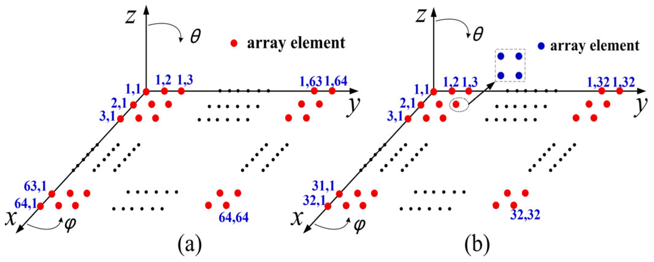
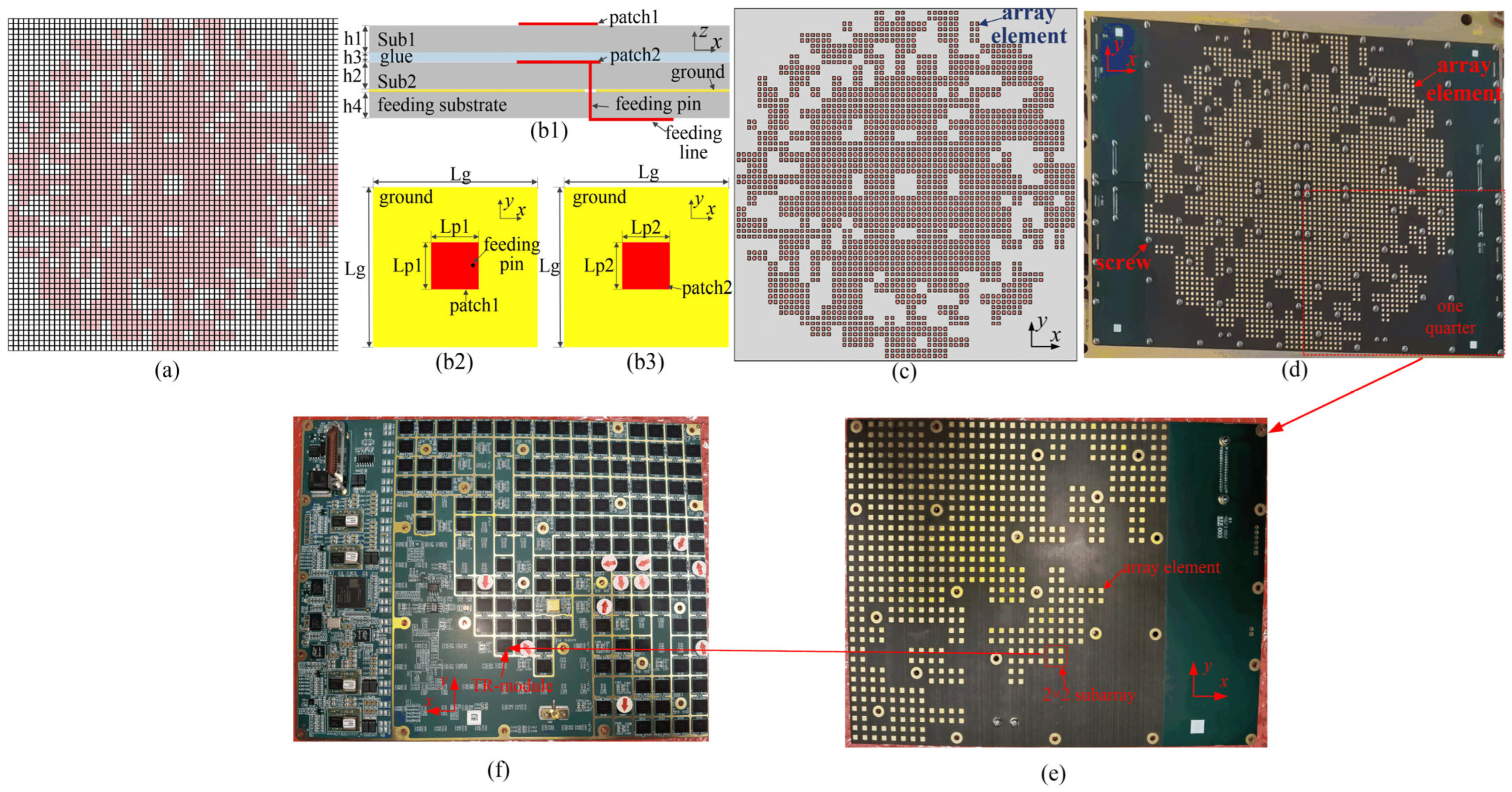
Based on the previous mathematical modeling and algorithm, the thinned array with a desired radiation pattern is achieved. In this section, the achieved array structure is first presented. Then, the array performance is shown for verification.

A.

Array Structure and Array Element

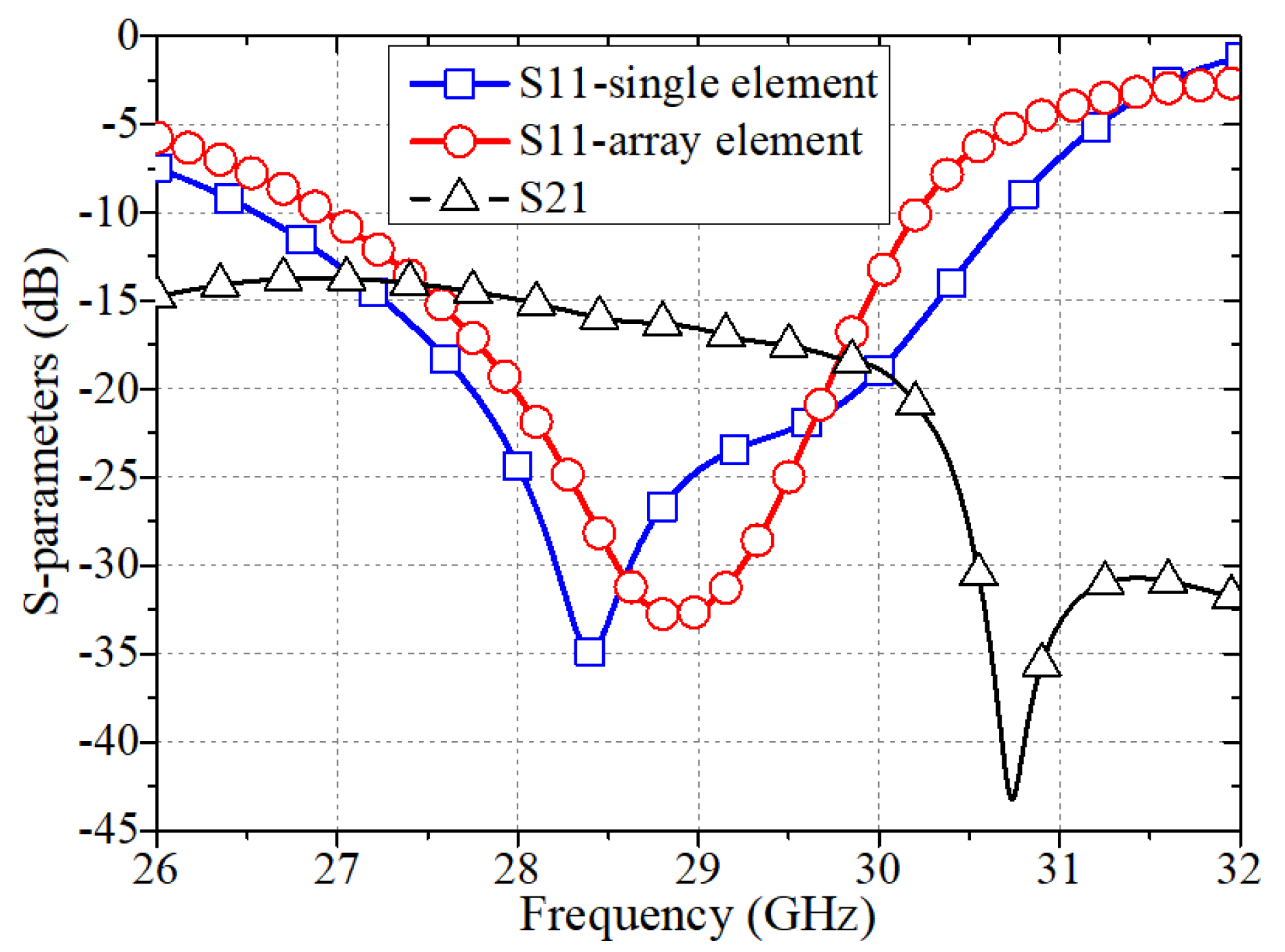
In accordance with the mathematical modeling and algorithm in Section 2, the optimized array structure of the large-scale 64 × 64 thinned array with 2400 elements is shown in Figure 2. As illustrated in Figure 2a, the full array is a 64 × 64 array with 4096 elements. The presence of a “red box” indicates an active element, while the presence of a “white box” means that there is no element. The total number of “red boxes” is 2400, which means that the thinned array has 2400 elements. Also, Figure 2a shows that every 2 × 2 element in the thinned array is a subarray.

To construct a thinned array, the array element was built first. The element was designed on three PCBs. The centers of the three PCBs are aligned. The substrate for the Sub1 and Sub 2 was Rogers RT5880 with a relative permittivity of 2.2 and a thickness of 0.381 mm. The substrate of the feeding structure was Rogers RT4003, with a relative permittivity of 3.5 and a thickness of 0.203 mm. Two rectangle patches, sized Lp1 = 2.4 mm and Lp2 = 2.6 mm, respectively, serving as the radiator, were etched onto the top layer of the Sub1 and Sub2, respectively. The Sub1 and Sub2 are bonded together using glue (prepreg layer). The glue was Rogers RO4350F with a relative permittivity of 3.52, a loss tangent of 0.004, and a thickness of h3 = 0.1 mm.

Based on the thinned array structure in Figure 2a and the array element in Figure 2b, a thinned array with 2400 elements was constructed, as shown in Figure 2c. The element spacings between each element were set to 5 mm. The proposed thinned array shown in Figure 2c was fabricated and is shown in Figure 2d. Several metal screws were used to align and fix the large-scale array. To better show the array, Figure 2d depicts the top-down view of the bottom-right quarter of the array. The array elements are on this layer. Figure 2e shows the back view of the bottom-right quarter of the array. The TR-modules are on this layer. Every 2 × 2 element of the array that is a subarray is directly fed by a TR module. Also, the TR modules have four output ports, which connect to the four ports of the 2 × 2 elements of the subarray directly.

B.

Performance of the Array Element

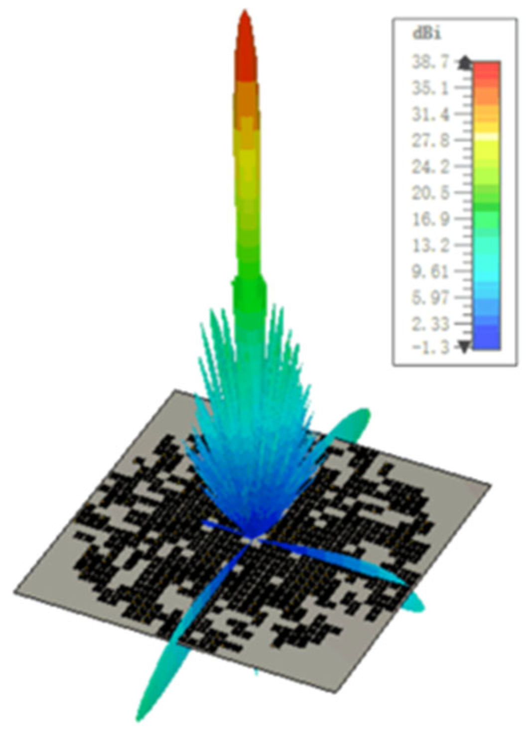
Figure 3 shows the simulated S-parameters of the array element in the cases of a single element (Figure 2b) and in the array (Figure 2c). In both cases, the overlapped −10 dB impedance bandwidth covers 3 GHz (27–30 GHz). The S11 in the cases of single element and in the array are similar. Additionally, the mutual coupling between each element in the array is lower than −14 dB. Figure 4 shows the simulated radiation patterns of the array element in the cases of single element (Figure 2b) and in the array (Figure 2c) at 29 GHz. For the two cases, the simulated gain is about 5.5 dBi. The cross-polarization level is lower than −25 dB and −15 dB for the case of the single element and the case in the array, respectively.

C.

Radiation Pattern of the Thinned Array

With the array structure in Figure 2a, the 2D normalized array factors of the large-scale thinned array with 2400 elements for the φ = 0°, φ = 45°, φ = 90°, and φ = 135° cut-planes are shown in Figure 5. From Figure 5, it can be seen that in the φ = 0°, φ = 45°, φ = 90°, and φ = 135° cut-planes, the radiation patterns in the sidelobe level regions meet the requirements. Figure 5a,c show that the first sidelobe levels are lower than −21.8 dB at the φ = 0° and φ = 90° cut-planes, while Figure 5b,d show that the first sidelobe levels are lower than −22.6 dB at the φ = 45° and φ = 135° cut-planes. To better illustrate the array factor, Figure 6 shows the 3D normalized array factor of the large-scale thinned array with 2400 elements. From Figure 6, it is apparent that, for each cut-plane with different azimuth angles, the gains at the sidelobe level regions are still small.

To verify the array factor, the radiation patterns of the array model in Figure 2c and the radiation patterns of the array prototype in Figure 2d are simulated and measured, respectively. The simulated 3D radiation pattern is shown in Figure 7. Figure 7 shows that the proposed thinned array can form a sharp beam with a high gain. The simulated and measured normalized radiation patterns in the φ = 0° and φ = 45° cut-planes are shown in Figure 8. From Figure 8, it is evident that the simulated radiation patterns match the array factor very well. The high sidelobe level at the large elevation angle might come from the radiation of the fringing field. Also, Figure 8 shows that the measured radiation patterns agree with the simulated ones. The slightly higher sidelobe level might come from the metal screws and the measured error.

In addition, because the array elements are large and the desired sidelobe level is complex, other methods, like nonlinear optimization methods (DE, PS, SA, IWO, or GA), decomposition, Fourier transform, etc., cannot easily converge. The present branch and bound technique with convex optimization is an efficient method for the synthesis of the large-scale thinned array with specific radiation pattern restrictions.

4. Conclusions

The synthesis of large-scale thinned arrays is a complex problem requiring precise convergence. This paper presents used the branch and bound technique with convex optimization for the synthesis of large-scale thinned arrays with low sidelobe levels. A total of 2400 elements were selected for the full 64 × 64 array with a sidelobe level that satisfies the system requirements. Simulated and measured results are presented to verify the design. The branch and bound with convex optimization technique can solve non-convex, mixed-integer, or combinatorial optimization problems, where convex relaxation is often applied to certain parts of the problem. This combination allows for the solving of problems that involve both discrete and continuous variables, especially where the continuous flexibility and adaptability of the branch and bound with convex optimization technique relaxation of a problem is convex. This method is versatile.

References

1. ITU, Vision, Requirements and Evaluation Guidelines for Satellite Radio Interface(s) of IMT-2020. ITU-R Report M.2514-0. 2022. Available online: https://rfi.colem.co.uk/wp-content/uploads/ITU-R-IMT-2020-Satellite-5G-6G-Vision-Enhanced-Mobile-Broadband-Massive-Machine-Ultra-reliable-Low-Latency-Comms.pdf (accessed on 3 December 2024).
2. 3GPP, Solutions for NR to Support Non-Terrestrial Networks (NTN). V16.2.0, Mar. 2023. 3rd Generation Partnership Project; Technical Specification Group Radio Access Network; NR; User Equipment (UE) Radio Transmission and Reception. Part 5: Satellite Access Radio Frequency (RF) and Performance Requirements (Release 18), Standard 3GPP TS 38.101-5 V18.4.0 (2023-12). Available online: https://www.etsi.org/deliver/etsi_ts/138100_138199/13810105/18.05.00_60/ts_13810105v180500p.pdf (accessed on 3 December 2024).
3. 3rd Generation Partnership Project; Technical Specification Group Radio Access Network; Study on New Radio (NR) to Support NonTerrestrial Networks (Release 15), Standard 3GPP TR 38.811 V15.4.0 (2020-09).
4. Hofmann, M. Satellite communication in the age of 5G. J. ICT Stand. 2020, 8, 247–252. [Google Scholar] [CrossRef]
5. Lin, S.; An, J.; Gan, L.; Debbah, M.; Yuen, C. Stacked intelligent metasurface enabled LEO satellite communications relying on statistical CSI. IEEE Wirel. Commun. Lett. 2024, 13, 1295–1299. [Google Scholar] [CrossRef]
6. Mailloux, R.J. Phased Array Antenna Handbook; Artech House: Norwood, MA, USA, 2005. [Google Scholar]
7. Balanis, C.A. Antenna Theory and Analysis and Design; John Wiley &Sons: Hoboken, NJ, USA, 2005. [Google Scholar]
8. Haupt, R.L. Adaptively thinned arrays. IEEE Trans Antennas Propag. 2015, 63, 1626–1632. [Google Scholar] [CrossRef]
9. Rocca, P. Large array thinning by means of deterministic binary sequences. IEEE Antennas Wirel. Propag. Lett. 2011, 10, 334–337. [Google Scholar] [CrossRef]
10. Gu, L.; Zhao, Y.-W.; Zhang, Z.-P.; Wu, L.-F.; Cai, Q.-M.; Hu, J. Linear array thinning using probability density tapering approach. IEEE Antennas Wirel. Propag. Lett. 2019, 18, 1936–1940. [Google Scholar] [CrossRef]
11. Wang, X.-K.; Jiao, Y.-C.; Tan, Y.-Y. Synthesis of large thinned planar arrays using a modified iterative Fourier technique. IEEE Trans Antennas Propag. 2014, 62, 1564–1571. [Google Scholar] [CrossRef]
12. Liu, Y.; Zheng, J.; Li, M.; Luo, Q.; Rui, Y.; Guo, Y.J. Synthesizing beam-scannable thinned massive antenna array utilizing modified iterative FFT for millimeter-wave communication. IEEE Antennas Wirel. Propag. Lett. 2020, 19, 1983–1987. [Google Scholar] [CrossRef]
13. Zhang, J.; Mao, X.; Zhang, M.; Hirokawa, J.; Liu, Q.H. Synthesis of thinned planar arrays based on precoded subarray structures. IEEE Antennas Wirel. Propag. Lett. 2023, 22, 44–48. [Google Scholar] [CrossRef]
14. Li, X.; Li, X.; Zhou, Z.; Zhang, C. Design and application of sparse array algorithm for Ka-band large-scale phased array. Telecommun. Eng. 2023, 63, 1524–1530. [Google Scholar]
15. Tian, X.; Wang, B.; Tao, K.; Li, K. An improved synthesis of sparse planar arrays using density-weighted method and chaos sparrow search algorithm. IEEE Trans. Antennas Propag. 2023, 71, 4339–4349. [Google Scholar] [CrossRef]
16. Goudos, S. Antenna design using binary differential evolution: Application to discrete-valued design problems. IEEE Antennas Propag. Mag. 2017, 59, 74–93. [Google Scholar] [CrossRef]
17. Jiang, H.; Gong, Y.; Zhang, J.; Dun, S. Irregular modular subarrayed phased array tiling by algorithm X and differential evolution algorithm. IEEE Antennas Wirel. Propag. Lett. 2023, 22, 1532–1536. [Google Scholar] [CrossRef]
18. Goudos, S.K.; Moysiadou, V.; Samaras, T.; Siakavara, K.; Sahalos, J.N. Application of a comprehensive learning particle swarm optimizer to unequally spaced linear array synthesis with sidelobe level suppression and null control. IEEE Antennas Wirel. Propag. Lett. 2010, 9, 125–129. [Google Scholar] [CrossRef]
19. Zhang, F.; Yang, X.; Huang, Q.; Tao, J. The optimization of uniform concentric ring array using improved simulated annealing algorithm. In Proceedings of the International Conference on Artificial Intelligence and Advanced Manufacturing (AIAM), Dublin, Ireland, 16–18 October 2019. [Google Scholar]
20. Li, S.; Wang, Y.; Xu, F. One-bit coding reconfigurable array for two-dimensional wide-angle scanning. IEEE Trans. Antennas Propag. 2023, 71, 2421–2432. [Google Scholar] [CrossRef]
21. Liu, G.; Zhu, H.; Wang, K.; Qiu, Y.; Mou, J.; Zheng, P.; Wei, G. Low-Sidelobe Pattern Synthesis for Sparse Conformal Arrays Based on Multiagent Genetic Algorithm. In Proceedings of the IEEE International Symposium on Antennas and Propagation and USNC-URSI Radio Science Meeting (AP-S/URSI), Denver, CO, USA, 10–15 July 2022. [Google Scholar]
22. Ha, B.V.; Mussetta, M.; Pirinoli, P.; Zich, R.E. Modified compact genetic algorithm for thinned array synthesis. IEEE Antennas Wirel. Propag. Lett. 2016, 15, 1105–1108. [Google Scholar] [CrossRef]
23. Shan, T.; Pan, X.; Li, M.; Xu, S.; Yan, F. Coding programmable metasurfaces based on deep learning techniques. IEEE J. Emerg. Sel. Top. Circuits Syst. 2020, 10, 114–125. [Google Scholar] [CrossRef]
24. Hong, Y.; Shao, W.; Lv, Y.-H.; Wang, B.-Z.; Peng, L.; Jiang, B. Knowledge-based neural network for thinned array modeling with active element patterns. IEEE Trans. Antennas Propag. 2022, 70, 11229–11234. [Google Scholar] [CrossRef]
Figure 1. Three-dimensional view of the full 64 × 64 array. (a) The full 64 × 64 array. (b) The full 32 × 32 array with a 2 × 2 subarray.
Electronics 14 00023 g001
Figure 2. Array structure and array element of the proposed thinned array. (a) Structure of the thinned array with 2400 elements (the “red box” represents the active element, and the “white box” represents no elements). (b) Structure of the array element: (b1) side view, (b2) top view of Sub1, and (b3) top view of Sub2; h1 = 0.381, h2 = 0.381, h3 = 0.1 mm, h4 = 0.203, Lp1 = 2.4, Lp2 = 2.6, Lg = 5, units: mm. (c) Model of the proposed thinned array with 2400 elements and an element spacing of 5 mm. (d) Fabricated prototype of the proposed thinned array with 2400 elements. (e) Top-down view of the bottom-right quarter of the array. (f) Bottom-up view of bottom-right quarter of the array.
Electronics 14 00023 g002
Figure 3. Simulated S-parameters of the array element in the cases of single element (Figure 2b) and in the array (Figure 2c).
Electronics 14 00023 g003
Figure 4. Simulated radiation patterns of the array element in the cases of single element (Figure 2b) and in the array (Figure 2c) at 29 GHz. (a) E-plane (xz-plane). (b) H-plane (yz-plane).
Electronics 14 00023 g004
Figure 5. Two-dimensional normalized array factor of the large-scale sparse array with 2400 elements. (a) φ = 0° cut-plane. (b) φ = 45° cut-plane. (c) φ = 90° cut-plane. (d) φ = 135° cut-plane.
Electronics 14 00023 g005
Figure 6. Three-dimensional normalized array factor of the large-scale thinned array with 2400 elements.
Electronics 14 00023 g006
Figure 7. Simulated 3D radiation patterns of the thinned array.
Electronics 14 00023 g007
Figure 8. Simulated and measured normalized radiation patterns of the thinned array in the φ = 0° and φ = 45° cut-planes. (a) φ = 0° cut-plane. (b) φ = 45° cut-plane.
Electronics 14 00023 g008
Disclaimer/Publisher’s Note: The statements, opinions and data contained in all publications are solely those of the individual author(s) and contributor(s) and not of MDPI and/or the editor(s). MDPI and/or the editor(s) disclaim responsibility for any injury to people or property resulting from any ideas, methods, instructions or products referred to in the content.