Whole-Body Control with Uneven Terrain Adaptability Strategy for Wheeled-Bipedal Robots

Abstract

Wheeled-bipedal robots (WBRs) integrate the locomotion efficiency and terrain adaptability of legged and wheeled robots. However, terrain adaptability is significantly influenced by the control system. This paper proposes a hierarchical control method for WBRs that includes an active force solver, a whole-body pose planner and a whole-body torque controller. The active force solver based on model predictive control (MPC) was constructed to calculate the active force from the wheeled legs to the torso to achieve the torso’s desired motion tasks. The whole-body pose planner based on the terrain adaptability strategy provides whole-body joint trajectories that can achieve dynamic balance and movement simultaneously without external sensing information. The whole-body torque controller is used to calculate whole-body joint torque based on the active force reference and joint motion reference. Finally, two simulation experiments were conducted to verify the effectiveness of the proposed method on uneven terrain.

1. Introduction

In recent years, mobile robots have been gradually applied to various fields of industry and life [1,2]. The ability of robots to adapt to different terrains has become a focus of research. Wheeled robots have high mobility efficiency on flat terrain [3], although their terrain adaptability is limited [4]. Legged robots have strong terrain adaptability and passage capabilities on uneven terrain [5,6,7,8,9] with low energy utilization efficiency [10,11]. To combine the advantages of both wheeled and legged robots, wheeled-bipedal robots (WBRs) have been developed [12]. WBRs enable fast movement over continuous flat and uneven terrain, with the legs acting as an active suspension system to ensure that torso movement tasks are accomplished [13].

WBRs are underdriven systems and are inherently unstable. Moving on uneven terrain is a challenge for WBRs. Handle is an excellent electro-hydraulic hybrid drive WBR that enables supple movements on uneven terrain, such as walking on grass and descending steps [14]. The WLR series of hydraulically driven wheeled humanoid robots from the Harbin Institute of Technology (HIT) uses a modeling approach based on the Two-Mass Spring-Damp Inverted Pendulum (TMS-DIP) model [15,16], which provides a high load capacity in complex environments and is capable of traversing rugged terrains and handling objects [17,18]. ETH Zurich developed a small WBR, Ascento [19], based on an assisted LQR whole-body control method [20] which can solve a set of desired joint accelerations, considering various motion tasks simultaneously. These desired joint accelerations are then converted to joint torques using a whole-body dynamics model. Xin S et al. [21] proposed an online dynamic motion planning and control method and implemented point-foot walking of the WBR in a simulation environment. Cao H et al. [22] presented a balance control strategy for wheeled bipedal robots on inclined surfaces, utilizing a model predictive controller (MPC) with input constraints and an extended state observer (ESO) to enhance robustness against unmodeled dynamics and external disturbances. Zhang J et al. [23] trained a balance controller in conjunction with a whole-body controller to control the robot Ollie to cross one-sided bridges, make a U-turn on a slope and drive downstairs. The balance control and motion control in the above methods are separate. The dynamic changes brought about by motion control are treated as disturbances by balance control, making it hard to fully exploit the robot’s locomotion potential. Chen Z et al. [24] presented an adaptive impedance control strategy for docking robots, addressing the issue of excessive collision contact force caused by environmental interference during autonomous docking tasks of unmanned ground vehicles. Xu Y et al. [25] proposed a dynamic localization framework based on asynchronous LiDAR–camera fusion to provide absolute attitude and position observations of UAVs, achieving robust localization and tracking in outdoor environments. In rehabilitation robotics or a hybrid robot design, Abbasimoshaei A et al. [26] presented the design of a one-degree-of-freedom device for paralyzed patients, focusing on wrist extension and flexion, utilizing a hydraulic actuator controlled by an impedance controller to assist in regaining mobility and independence. For robots, according to different motion tasks and different application scenarios, different control algorithms can be used to achieve different results, which makes the control algorithm a very important part of the robot design process.

To some extent, the modeling method of WBRs is the foundation of the control framework [27,28]. The modeling approaches in the above methods are the wheeled inverted pendulum virtual model combined with the whole-body dynamics model. Inspired by [29,30,31], distributed dynamics modeling is employed to describe WBRs, and this paper proposes a hierarchical control method for WBRs that includes an active force solver, a whole-body pose planner and a whole-body torque controller. The active force solver based on model predictive control (MPC) is constructed to calculate the active force from the wheeled legs to the torso to achieve the torso’s desired motion tasks. The whole-body pose planner based on the terrain adaptability strategy provides whole-body joint trajectories that can achieve dynamic balance and movement simultaneously based on internal sensing information. The whole-body torque controller is used to calculate whole-body joint torque based on the active force reference and joint motion reference. Based on this control method, when the terrain height and angle change continuously, the feedback signals from internal sensors will affect the length and tilt angle of the two wheeled legs, thus ensuring the motion of the torso with respect to the posture. The main contributions are outlined below.

(1) The balance task is transformed into a joint motion task using a whole-body pose planner so that all body joints can be used for balance adjustment, thus improving balance. Based on this, a model-based predictive control algorithm transforms the torso’s desired motion into the active force of the wheeled legs on the torso. Therefore, when the robot moves on uneven terrain, the torque of the whole body can be adjusted to maintain the consistency of the torso’s motion and the balancing task.

(2) Carrying out balancing and locomotion tasks through force control allows the robot to better adapt to different environmental conditions and different contact situations.

This paper is organized into the following sections: Section 2 introduces the basic parameters of WBRs and defines the coordinate system. Section 3 describes the whole-body dynamics modeling process for WBRs. Section 4 describes the construction of the control framework of WBRs. Section 5 presents the simulation experiments and analyzes the results. Finally, Section 6 summarizes the paper.

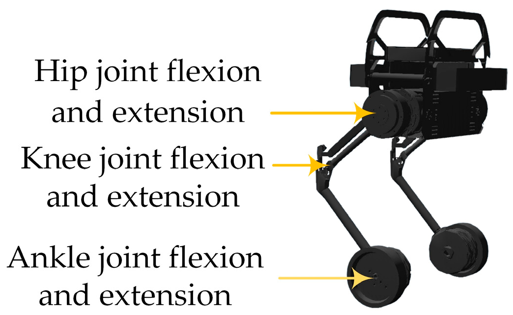
2. Robot Basic Information

Skater-I (shown in Figure 1), which is the focus of this paper, consists of a torso and two wheeled legs. Each wheeled leg has three pitch joints connecting the torso, thigh, calf and wheel.

Skater-I has its hip motors and knee motors arranged at the hip joints, and the batteries and controllers are mounted inside the torso shell, so the combined mass of the right and left hip joints, knee motors and torso is recorded as $m_b$ = 6.728 kg as the total mass of the torso, and the other parameter values are shown in

Table 1. Skater-I component parameter table.

Component Name	Parameter Name	Parameter Values	Parameter Name	Parameter Values
Thigh	$L_1$	0.21 m	$m_1$	1 kg
Calf	$L_2$	0.24 m	$m_2$	0.73 kg
Wheel	$r_W$	0.04 m	$m_w$	0.59 kg

and

Table 2. Skater-I motor parameter table.

Component Name	Maximum Torque	Joint Range of Motion
Hip motors	$24 \mathrm{N}\cdot \mathrm{m}$	[−0.2 rad, 1 rad]
Knee motors	$24 \mathrm{N}\cdot \mathrm{m}$	[−2.1 rad, −1 rad]
Wheel joint motors	$8.3 \mathrm{N}\cdot \mathrm{m}$	——

. Skater-I has no external sensors and now contains only internal sensors, and the sensor locations and sensor types are shown in

Table 3. Sensor information for Skater-I.

Sensor Position	Sensor Type
Skater-I center of mass position Hip position	IMU sensors Position sensor
Knee position	Position sensor
Ankle position	Position sensor

. The IMU sensors provide the robot’s roll, pitch and yaw angles, and the position sensors in the wheel and leg joints are used to calculate the rotation angles of the hip, knee and ankle joints.

The definition of the coordinate system is shown in Figure 2, where ${\sum }_I$ is a fixed coordinate system, the origin is at the center of the two wheels in the initial position, the positive direction of the $x$ axis points to the horizontal forward direction of the starting position, the positive direction of the $z$ axis is opposite to the direction of gravity and the positive direction of the $y$ axis is obtained by using the right-hand rule. ${\sum }_n$ is the following coordinate system, the origin is at the center of mass of the torso and the direction of the coordinate system is the same as that of the ${\sum }_I$ coordinate system. ${\sum }_b$ is the following coordinate system,; the origin is at the center of mass of the torso; the $x$, $y$ and $z$ axes point to the front, left and upper sides of the torso, respectively; and the angles represented by ${\sum }_n$ are the roll angle $\alpha$, the pitch angle $\beta$ and the yaw angle $\gamma$, respectively.

3. Dynamical Modeling

As shown in Figure 3, Skater-I is a typical floating base system where the torso is driven by the active force provided by the wheeled legs. The whole-body dynamics model of WBRs is constructed by constructing a single stiff-body dynamics model of the torso and a wheeled-leg dynamics model and combining the force transfer relationship between the torso and the wheeled legs. As a result, we designed and built the single rigid-body dynamics model of the torso to be driven by the active force and the wheeled-leg dynamics model to be driven by the joint torque.

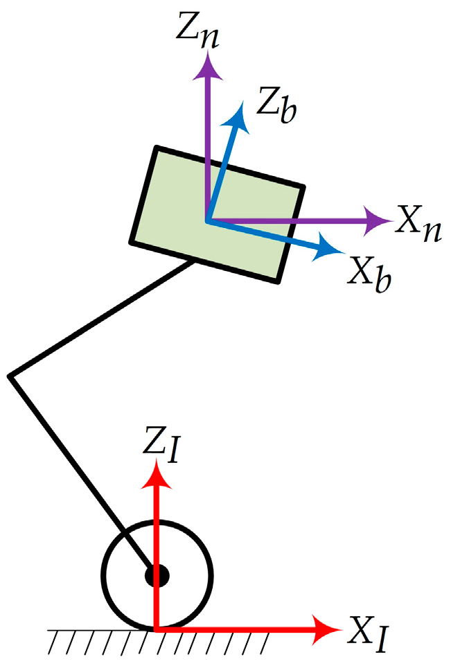
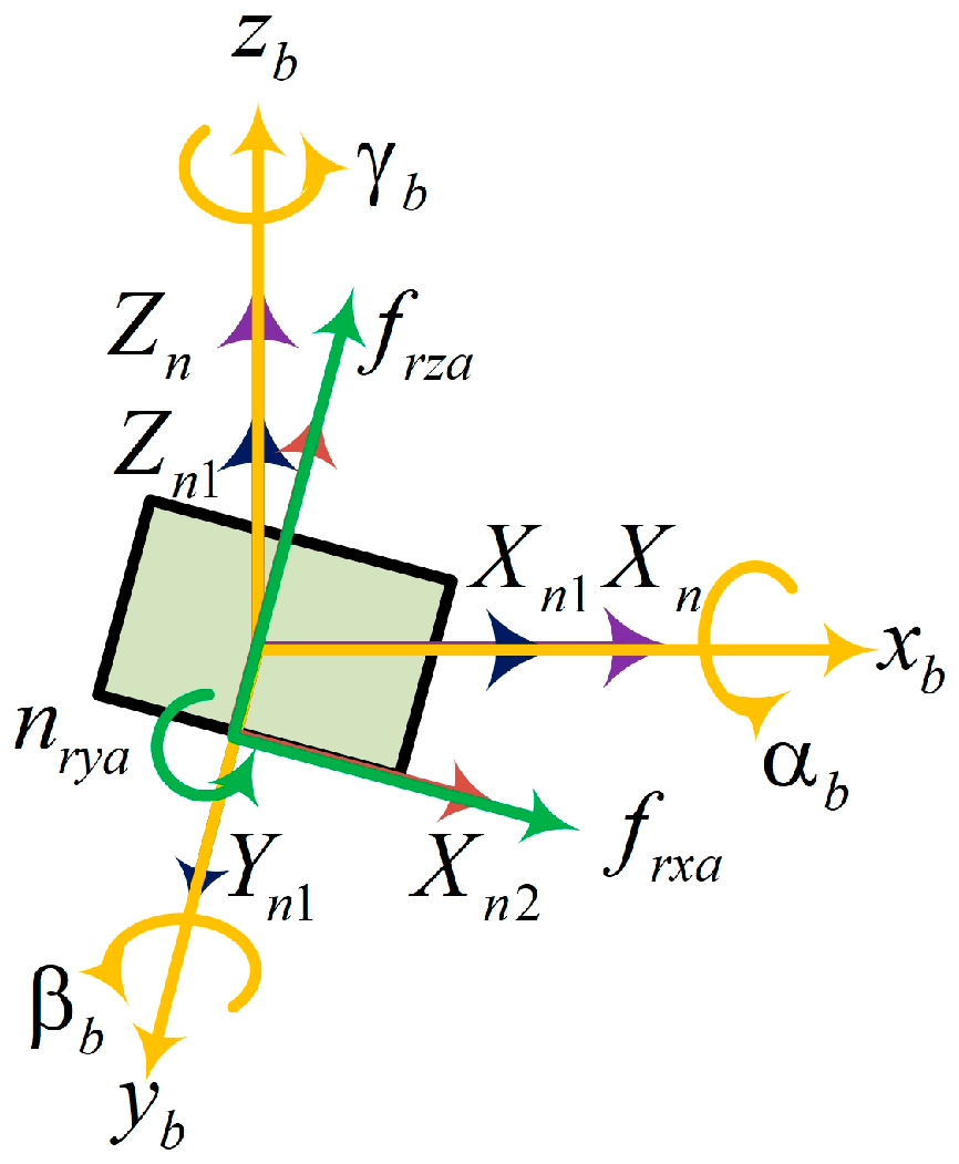
3.1. Single Rigid-Body Model of Torso

We can define the active driving force provided by the left and right wheeled-leg systems on the torso system as $W_{ia}={\left[\hspace{0.17em}{f}_{ixa}\hspace{1em}{f}_{iza}\hspace{0.17em}\hspace{1em}{n}_{iya}\hspace{0.17em}\right]}^T$, where $i=l or r$, as shown in Figure 4, the positive directions of $f_{ixa}$, $f_{iza}\hspace{0.17em}$ and $n_{iya}$ are the positive directions of the $x$ axis of the ${\sum }_{n2}$ coordinate system, the positive direction of the $z$ axis of the ${\sum }_{n2}$ coordinate system and the direction of the ${\sum }_{n2}$ coordinate system rotating around the positive direction of the $y$ axis, respectively. The angle between ${\sum }_{n2}$ and ${\sum }_n$ is the angle between the roll angle $\alpha$ and the pitch angle $\beta$. Therefore, the driving force on the single rigid body of the torso is $W_a={\left[\hspace{0.17em}{W}_{ra}\hspace{1em}{W}_{la}\hspace{0.17em}\right]}^T$.

WBRs move in 3D space using six-dimensional vectors to describe the position and attitude of the torso, and the resulting generalized positions and velocities are given in Equation (1):

$$q_b=\left[\begin{array}{l}\hspace{0.17em}{p}_b\hspace{0.17em}\\ \hspace{0.17em}{\Theta }_b\end{array}\right]\hspace{1em}\hspace{1em}{\dot{q}}_b=\left[\begin{array}{l}\hspace{0.17em}{V}_b\hspace{0.17em}\\ \hspace{0.17em}{\omega }_b\hspace{0.17em}\end{array}\right]$$

(1)

where $p_b\in {\left[x_b,y_b,z_b\right]}^T$ represents the position of the torso, as shown in Figure 4, and the positive directions of $x_b$, $y_b$ and $z_b$ are the same as the positive directions of the ${\sum }_{n1}$ coordinate system’s $x$ axis, $y$ axis and $z$ axis, respectively. ${\Theta }_b\in {\left[{\alpha }_b,{\beta }_b,{\gamma }_b\right]}^T$ represents the attitude of the torso, and the positive directions of ${\alpha }_b$, ${\beta }_b$ and ${\gamma }_b$ are the counterclockwise rotation directions of the ${\sum }_I$ coordinate system around the $x$ axis, $y$ axis and $z$ axis, respectively. The angle between ${\sum }_{n1}$ and ${\sum }_n$ is the yaw angle $\gamma$. $V_b\in \left[v_b,{\dot{y}}_b,{\dot{z}}_b\right]$ and ${\omega }_b\in {\left[{\dot{\alpha }}_b,{\dot{\beta }}_b,{\dot{\gamma }}_b\right]}^T$ represent the linear and angular velocities of the torso.

The dynamics of the torso subsystem are modeled as follows:

$$\left\{\begin{array}{l}{}^{n1}\ddot{p}_b={\displaystyle \frac{{\displaystyle {\sum }_{i=l,r}{}^{n1}F_{ia}}}{m_b}}+{}^{n1}G\\ {\displaystyle \frac{d\left({}^{n}I_b{}^n\omega _b\right)}{dt}}\approx {}^{n}I_b{}^n\dot{\omega }_b={\displaystyle {\sum }_{i=l,r}\left({}^{n}r_i\times {}^{n}F_{ia}+{}^{n}n_{ia}\right)}\end{array}\right.$$

(2)

where ${}^{n1}F_{ia}\hspace{0.33em}\hspace{0.33em}=\hspace{0.33em}{}_{n2}{}^{n1}R\hspace{0.33em}{\left[f_{ixa} 0 f_{iza}\right]}^T$, ${}^{n}n_{ia}\hspace{0.33em}\hspace{0.33em}=\hspace{0.33em}\hspace{0.33em}{}_{n2}{}^{n}R{\left[0 n_{iya} 0\right]}^T$, ${}^{n}F_{ia}={}_{n2}{}^{n}R\hspace{0.33em}{\left[f_{ixa} 0 f_{iza}\right]}^T$, and ${}^{n1}G\hspace{0.33em}\hspace{0.33em}=\hspace{0.33em}\hspace{0.33em}{\left[0 0 g\right]}^T$ denote the gravitational acceleration vector, ${}^{n}I_b\in {ℝ}^{3\times 3}$ denotes the inertia tensor matrix of the torso in ${\sum }_n$ and ${}^{n}r_i\in {ℝ}^3$ denotes the vector from the center of mass of the torso to the hip joint in ${\sum }_n$, where ${}_{n2}{}^{n1}R$ and ${}_{n2}{}^{n}R$ are the descriptions of ${\sum }_{n2}$ relative to ${\sum }_{n2}$ and ${\sum }_{n2}$ relative to ${\sum }_n$, respectively. Equation (2) establishes the relationship between the torso position and the active driving force provided by the wheeled leg on the torso.

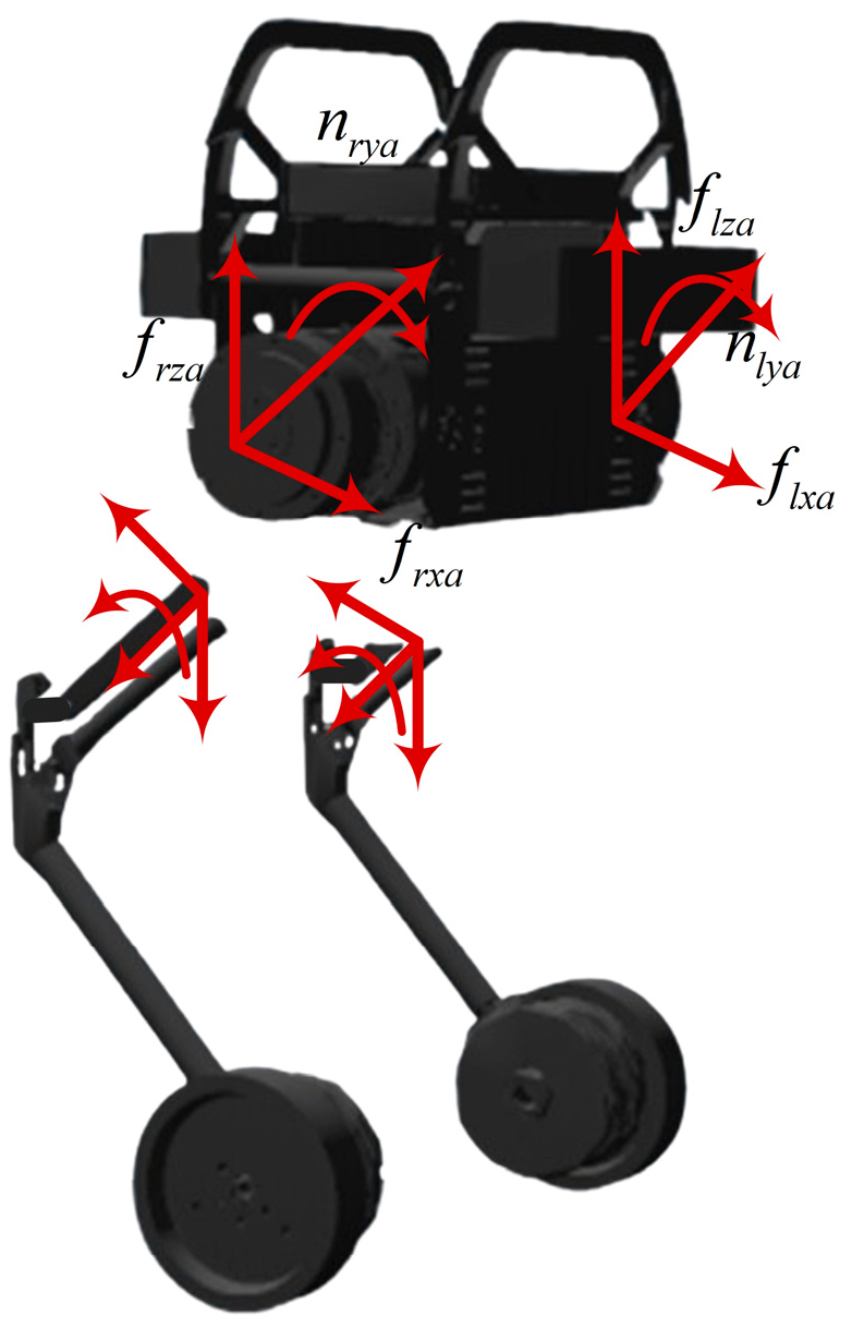
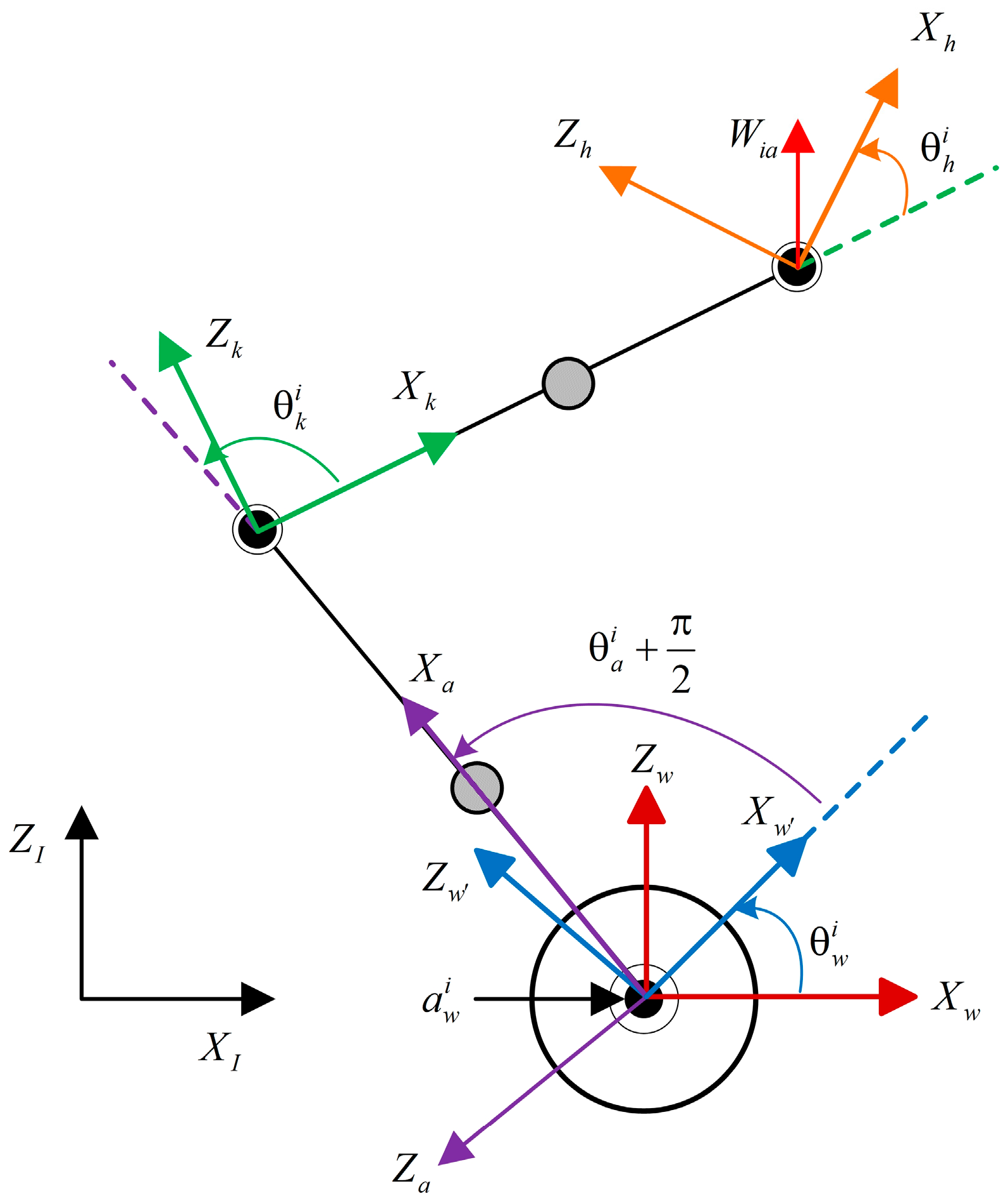
3.2. Wheeled Leg Integration Model

The unilateral wheeled leg is treated as a subsystem, and the dynamics of the wheeled-leg system are modeled with the wheel as the dynamic basis. Based on this model, the effect of underdrive characteristics on the end output force (the torso is subjected to an active driving force) can be eliminated.

Under the coordinate system ${\Sigma }_I$, the coordinate system setting and joint space selection of each rod of the unilateral wheeled leg are shown in Figure 5. The angle of rotation of the follower coordinate system ${\Sigma }_{w^{\prime }}$, which is fixed to the wheel, with respect to the fixed coordinate system ${\Sigma }_w$ is ${\theta }_w^i$; the angle of rotation of the coordinate system ${\Sigma }_a$ fixed to the calf with respect to the coordinate system ${\Sigma }_{w^{\prime }}$ is defined as ${\theta }_a^i+\pi /2$, where ${\theta }_a^i$ is the ankle joint angle, the angle at which the thigh bar is attached to coordinate system ${\Sigma }_k$ relative to coordinate system ${\Sigma }_a$ is the knee angle ${\theta }_k^i$ and the initial position of the coordinate system ${\Sigma }_h$ attached to the hip joint is the same as that of coordinate system ${\Sigma }_k$, and the angle ${\theta }_h^i$ between the two coordinate systems is the hip angle.

${\theta }_w^i$ is the initial state provided by the moving base, as shown in Equation (3):

$$\left\{\begin{array}{l}{}^0\omega _w^i=\hspace{0.17em}\hspace{0.17em}{\left[\begin{array}{ccc}0& 0& {\dot{\theta }}_w^i\end{array}\right]}^{{\rm T}}\\ {}^0\dot{\omega }_w^i=\hspace{0.17em}\hspace{0.17em}{\left[\begin{array}{ccc}0& 0& {\ddot{\theta }}_w^i\end{array}\right]}^{{\rm T}}\\ {}^0\dot{v}_w^i=\hspace{0.17em}\hspace{0.17em}{\left[\begin{array}{c}\cos {\theta }_w^i{a}_w^i\hspace{0.17em}\hspace{0.17em}+\hspace{0.17em}\hspace{0.17em}\sin {\theta }_w^{i}g-\sin {\theta }_w^i{a}_w^i\hspace{0.17em}\hspace{0.17em}+\hspace{0.17em}\hspace{0.17em}\cos {\theta }_w^{i}g\hspace{1em}0\end{array}\right]}^{{\rm T}}\end{array}\right.$$

(3)

where ${}^0\mathit{\omega }_w^i$, ${}^0\dot{\mathit{\omega }}_w^i$ and ${}^0\dot{\mathit{v}}_w^i$ denote the initial angular velocity, angular acceleration and linear acceleration of the movable base, respectively, and $a_w^i$ is the acceleration of the wheel’s movable base moving along the $x$ axis of the coordinate system ${\Sigma }_I$.

The left and right wheeled legs were analyzed separately, and the joint angle of the wheeled-leg system was defined as $q_j$, the joint angular velocity as ${\dot{q}}_j$ and the driving torque as $\tau$:

$$\begin{array}{l}{q}_j={\left[q_{wheel}\hspace{1em}{q}_{leg}\right]}^T={\left[{\theta }_a^r\hspace{1em}{\theta }_a^l\hspace{1em}{\theta }_k^r\hspace{1em}{\theta }_h^r\hspace{1em}{\theta }_k^l\hspace{1em}{\theta }_h^l\right]}^T\\ {\dot{q}}_j={\left[{\dot{q}}_{wheel}\hspace{1em}{\dot{q}}_{leg}\right]}^T={\left[{\dot{\theta }}_a^r\hspace{1em}{\dot{\theta }}_a^l\hspace{1em}{\dot{\theta }}_k^r\hspace{1em}{\dot{\theta }}_h^r\hspace{1em}{\dot{\theta }}_k^l\hspace{1em}{\dot{\theta }}_h^l\right]}^T\\ \tau ={\left[{\tau }_{wheel}\hspace{1em}{\tau }_{leg}\right]}^T={\left[{\tau }_w^r\hspace{1em}{\tau }_w^l\hspace{1em}{\tau }_k^r\hspace{1em}{\tau }_h^r\hspace{1em}{\tau }_k^l\hspace{1em}{\tau }_h^l\right]}^T\end{array}$$

(4)

According to Equations (3) and (4), the wheeled-legged subsystem is modeled based on the Newton–Euler iterative dynamics algorithm, and the standard form of its dynamics model is shown in Equation (5):

$$M\left(q_j,{\theta }_w\right){\ddot{q}}_j+C\left(q_j,{\dot{q}}_j,{\theta }_w,{\dot{\theta }}_w\right)+G\left(q_j,{\theta }_w\right)+I\left({\theta }_w,{\dot{\theta }}_w\right)a_w+J^{{\rm T}}{W}_a=\tau$$

(5)

where $M\in {ℝ}^{6\times 6}$, $C\in {ℝ}^{6\times 1}$ and $G\in {ℝ}^{6\times 1}$ are the inertia matrix, the Koch force and centrifugal force vectors, and the gravity vector, respectively. $I\in {ℝ}^{6\times 4}$ is the dynamic base inertial force compensation vector. $a_w={\left[a_w^r\hspace{1em}{\ddot{\theta }}_w^r\hspace{1em}{a}_w^l\hspace{1em}{\ddot{\theta }}_w^l\right]}^{{\rm T}}$. $J\in {ℝ}^{6\times 6}$ is the generalized Jacobi matrix. Equation (5) establishes mapping between the active driving force $W_a$ supplied by the wheeled leg on the torso and the joint torque $\tau$ in the wheeled-legged subsystem.

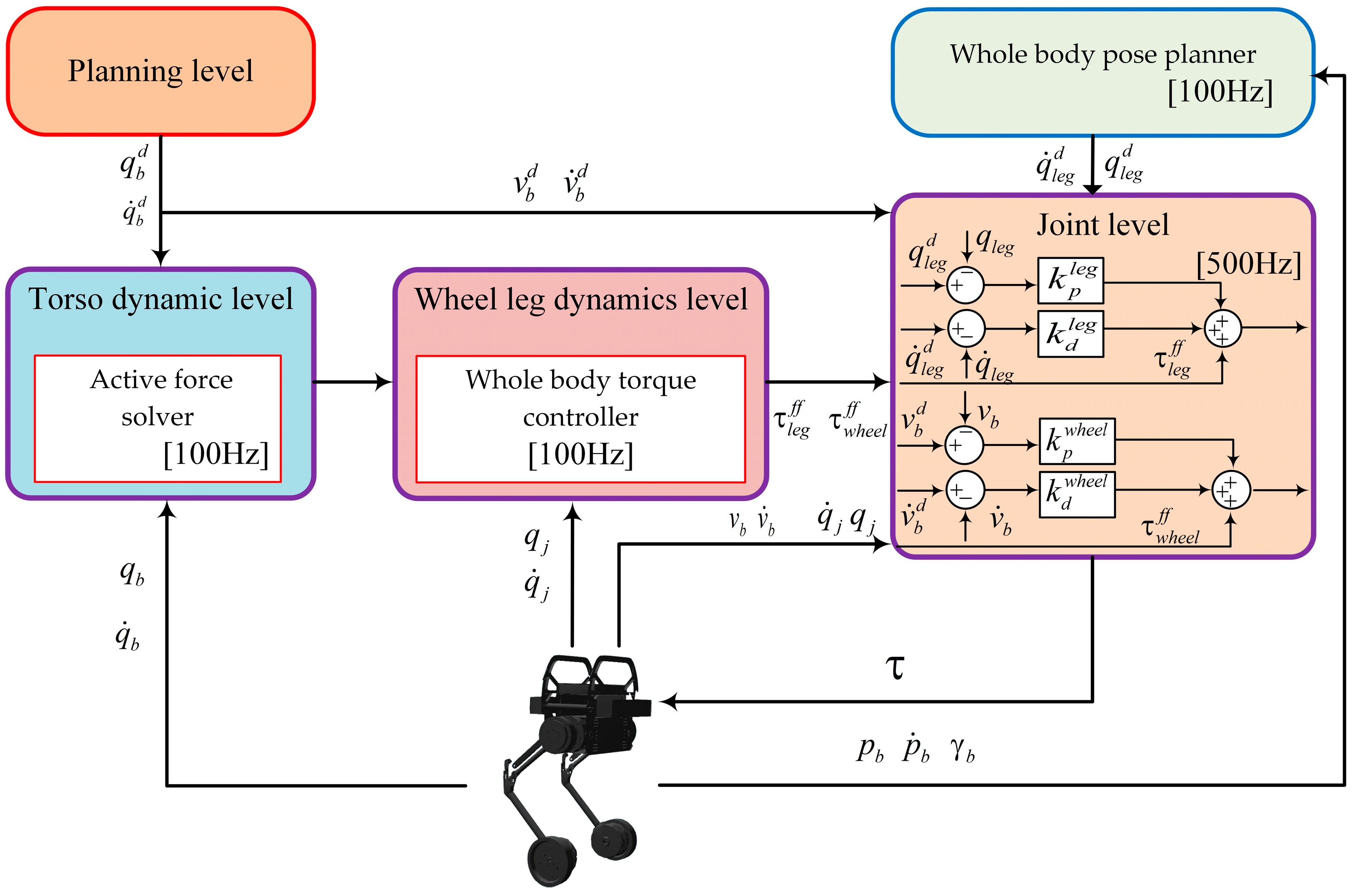
4. Control Framework Construction

This section proposes a whole-body control method with an uneven terrain adaptability strategy, as shown in Figure 6. There are three parts: the active force solver, the whole-body pose planner and the whole-body torque controller. Firstly, the active force solver based on model predictive control is constructed to solve the active force required for the torso movement. Secondly, the dynamic balance posture of the wheeled legs is planned by the whole-body pose planner based on the torso’s desired pose and the real pose. Finally, the whole-body torque controller is utilized to convert the active driving force and desired joint trajectory into the wheeled leg joint torque.

4.1. Active Force Solver Based on Model Predictive Control

We define $x^{\prime }={\left[\hspace{0.17em}{x}_b\hspace{1em}{z}_b\hspace{1em}\alpha \hspace{1em}\beta \hspace{1em}\gamma \hspace{1em}{v}_b\hspace{1em}{\dot{z}}_b\hspace{1em}\dot{\alpha }\hspace{1em}\dot{\beta }\hspace{1em}\dot{\gamma }\hspace{0.17em}\right]}^T$ as the state variable, define $u={[F_{rxa},\hspace{0.33em}\hspace{0.33em}{F}_{rza},\hspace{0.33em}\hspace{0.33em}{N}_{rza},\hspace{0.33em}\hspace{0.33em}{F}_{lxa},\hspace{0.33em}\hspace{0.33em}{F}_{lza},\hspace{0.33em}\hspace{0.33em}{N}_{lza}]}^T$ as the input to the state equation and write the torso dynamics model (Equation (2)) in the form of a state space equation, as shown in Equation (6):

$${\dot{x}}^{\prime }=A^{\prime }{x}^{\prime }+B^{\prime }u+G^{\prime }$$

(6)

where $A^{\prime }\in {ℝ}^{10\times 10}$ is the state matrix of the torso subsystem, $B^{\prime }\in {ℝ}^{10\times 6}$ is the input matrix of the torso subsystem and $G^{\prime }={ℝ}^{10\times 1}$ is the gravity vector. After expanding the state variable $x^{\prime }$ to $x={\left[\hspace{0.17em}{x}^{\prime }\hspace{1em}g\hspace{0.17em}\right]}^T$, the standard state space expression is obtained as shown in Equation (7):

$$\dot{x}=Ax+Bu$$

(7)

where the number of state variables is $n=11$, $A\in {ℝ}^{11\times 10}$ is the state matrix of the torso subsystem and $B\in {ℝ}^{11\times 6}$ is the input matrix of the torso subsystem. To simplify the solution, we discretize a time-varying state-space expression into a discrete-time state-space expression using a zero-order keeper:

$$x(k+1)=A_{d}x(k)+B_{d}u(k)$$

(8)

where $A_d=e^{A\Delta t}$ denotes the discrete state matrix, $B_d=B{\displaystyle {\int }_0^{\Delta t}{e}^{A\Delta t}}dt$ denotes the discrete input matrix and $\Delta t$ is the discrete period, which is also the sampling period of the hierarchical control framework.

Based on Equation (8), the torso state from moment $k$ to moment $k+N_p$ is predicted as shown in Equation (9):

$$\begin{array}{l}X\left(k\right)=Fx\left(k\right)+\Phi U\left(k\right)\\ X\left(k\right)={\left[x{\left(k+1\left|k\right.\right)}^T,x{\left(k+2\left|k\right.\right)}^T,\cdots ,x{\left(k+N_p\left|k\right.\right)}^T\right]}^T\\ U\left(k\right)\triangleq {\left[u{\left(k\left|k\right.\right)}^T,u{\left(k+1\left|k\right.\right)}^T,\cdots ,u{\left(k+N_c\left|k\right.\right)}^T\right]}^T\end{array}$$

(9)

$$\begin{array}{l}F={\left[A^T\hspace{1em}\hspace{1em}\hspace{1em}\hspace{0.17em}\hspace{0.17em}\hspace{0.17em}\hspace{0.17em}\hspace{0.17em}\hspace{0.17em}{\left(A^2\right)}^T\hspace{1em}\hspace{1em}\cdots \cdots \hspace{1em}\hspace{1em}\hspace{1em}{\left(A^{N_p}\right)}^T\right]}^T\\ \Phi =\left[\begin{array}{l}\hspace{1em}{B}_b\hspace{1em}\hspace{1em}\hspace{1em}\hspace{0.17em}\hspace{0.17em}\hspace{0.17em}\hspace{0.17em}\hspace{0.17em}0\hspace{1em}\hspace{1em}\hspace{1em}\hspace{0.17em}\cdots \hspace{1em}\hspace{1em}\hspace{0.17em}\hspace{0.17em}\hspace{1em}\hspace{0.17em}\hspace{0.17em}\hspace{1em}0\\ \hspace{0.17em}\hspace{0.17em}{A}_b{B}_b\hspace{1em}\hspace{1em}\hspace{0.17em}\hspace{0.17em}\hspace{0.17em}\hspace{0.17em}\hspace{0.17em}\hspace{0.17em}{B}_b\hspace{1em}\hspace{1em}\hspace{1em}\cdots \hspace{1em}\hspace{1em}\hspace{0.17em}\hspace{0.17em}\hspace{0.17em}\hspace{1em}\hspace{0.17em}\hspace{1em}0\\ \hspace{1em}\hspace{1em}\hspace{1em}\hspace{1em}\hspace{1em}\hspace{1em}\hspace{0.17em}\hspace{0.17em}⋮\\ {A_b}^{N_c-1}{B}_b\hspace{1em}\hspace{1em}{A_b}^{N_c-2}{B}_b \hspace{0.17em}\hspace{0.17em}\hspace{0.17em}\hspace{0.17em}\cdots \hspace{1em}\hspace{1em}\hspace{1em}\hspace{1em}\hspace{1em}{B}_b\\ \hspace{1em}\hspace{1em}\hspace{1em}\hspace{1em}\hspace{1em}\hspace{1em}\hspace{0.17em}\hspace{0.17em}⋮\\ {A_b}^{N_p-1}{B}_b\hspace{1em}\hspace{1em}{A_b}^{N_p-2}{B}_b \hspace{0.17em}\hspace{0.17em}\hspace{0.17em}\hspace{0.17em}\cdots \hspace{1em}\hspace{1em}{A_b}^{N_p-N_c}{B}_b\end{array}\right]\end{array}$$

(10)

where $F\in {ℝ}^{n*N_p\times n*N_p}$ and $\Phi \in {ℝ}^{6N_p\times 6N_c}$. $N_c$ and $N_p$ are the control time domain and prediction time domain, respectively, $N_c\le N_p$ $x\left(k+i\left|k\right.\right)$ represents the state of the trunk subsystem at the moment of $k$ predicted by the discrete state-space equations at the moment of $k+i$, and $u\left(k+i\left|k\right.\right)$ represents the system input at the moment of $k$ predicted by the discrete state-space equations at the moment of $k+i$.

With the objective of minimizing the error between the actual motion state of the torso and the desired motion state, and considering the magnitude of the desired driving force $U\left(k\right)$, the cost function at the moment of $k$ is constructed as shown in Equation (11):

$$J\left(k\right)={‖X(k)-X^d\left(k\right)‖}_{Q^{\ast }}+{‖U\left(k\right)‖}_{R^{\ast }}$$

(11)

where $X^d\left(k\right)={\left[{\left(x^d\left(k+1\right)\right)}^T,{\left(x^d\left(k+2\right)\right)}^T,\cdots ,{\left(x^d\left(k+N_p\right)\right)}^T\right]}^T$ denotes the desired state of the trunk posture from moment $k+1$ to moment $k+N_p$, $Q^{\ast }\in {ℝ}^{N_p\times N_p}$ is a positive definite diagonal matrix representing the weight matrix of the trunk system state error from moment $k+1$ to moment $k+N_p$ and $R^{\ast }\in {ℝ}^{N_p\times N_c}$ is a semi-positive definite diagonal matrix representing the weight matrix of the trunk subsystem input from moment $k+1$ to moment $k+N_p$.

As shown in Table 1, the maximum torque of the hip joint motors of the WBRs is 24 $\mathrm{N}\cdot \mathrm{m}$, and the upper and lower bounds of the input variables of the torso subsystem are set as shown in Equation (12):

$${[-100-100-24]}^T\le u\left(k+i\left|k\right.\right)\le {[100 100 24]}^T,i=0,1,2,\cdots ,N_{c-1}$$

(12)

We write Equation (12) in the standard form, $\underset{\_}{U}\le U\left(k\right)\le \overline{U}$, where $\underset{\_}{U}$ and $\overline{U}$ represent the upper and lower bounds of the torso driving force from moment $k$ to moment $k_{N_c-1}$, respectively. In order to ensure that the obtained driving force satisfies the ground friction cone constraint and no sliding occurs between the wheel and the ground, we set the friction cone constraint as $\left|F_{rx}+F_{lx}\right|\le \mu \left|F_{rz}+F_{lz}\right|$, where $\mu$ is the friction coefficient, and all the inequality constraints can be converted to the standard form, as shown in Equation (13):

$$A_{u}U\left(k\right)\le b_u$$

(13)

where $A_u$ is the coefficient matrix of the inequality constraint, and $b_u$ is the constant vector of the inequality constraint.

According to Equations (11)–(13), the problem of solving the cost function $J$ can be converted into a standard quadratic programming solution problem at the time of $k$, as shown in Equation (14):

$$\begin{array}{l}\underset{U\left(k\right)}{\min }\hspace{0.33em}\hspace{1em}{\displaystyle \frac{1}{2}}U{\left(k\right)}^{T}HU\left(k\right)+g^{T}U\left(k\right)\\ s.t\hspace{1em}\hspace{1em}\hspace{1em}{A}_{u}U\left(k\right)\le b_u\\ \hspace{1em}\hspace{1em}\hspace{1em}\hspace{1em}\underset{\_}{U}\le U\left(k\right)\le \overline{U}\end{array}$$

(14)

During the writing of the WBR hierarchical control framework project, we add the C++ tripartite library QPOASES and utilize the API in QPOASES (“QProblem.getPrimalSolution()”) to solve for Equation (14), and then the optimal control sequence $U\left(k\right)$ for the torso subsystem at moment $k$ can be solved. As a result, at moment $k$, the active drive of the wheeled legs to the torso $W_a$ is shown in Equation (15):

$$W_a=\left[E_{6\times 6},0,\cdots ,0\right]U\left(k\right)$$

(15)

4.2. Whole-Body Pose Planner with Terrain Adaptability Strategy

During the passage of WBRs on uneven terrain, as shown in Figure 7, the roll angle ${\alpha }_b$ of the torso will change frequently due to the different longitudinal slopes and absolute heights of the terrain where the left and right wheels are located, the expected wheel–ground contact point coordinates and expected wheel axis coordinates are calculated in real time using the coordinate system ${\sum }_{\mathrm{b}}$, and the contact point coordinates are mapped to the expected joint angles and expected joint angular velocities of the wheeled leg joints by combining wheeled leg inverse kinematics and joint angular velocities to maintain a stable robot posture and enhance the ability of WBRs to move on uneven terrain.

In coordinate system ${\sum }_b$, the coordinates of the wheel–ground contact point at the moment of $k$ are defined as $p_{wp}\left(k\right)={\left[z_{wp}^r\left(k\right)\hspace{1em}{x}_{wp}^r\left(k\right)\hspace{1em}{z}_{wp}^l\left(k\right)\hspace{1em}{x}_{wp}^l\left(k\right)\right]}^T$, and the coordinates of the desired wheel–ground contact point at the moment of $k$ are defined as $p_{wp}^d\left(k+1\right)={\left[{}^{d}z_{wp}^r\left(k+1\right)\hspace{1em}{}^{d}x_{wp}^r\left(k+1\right)\hspace{1em}{}^{d}z_{wp}^l\left(k+1\right)\hspace{1em}{}^{d}x_{wp}^l\left(k+1\right)\right]}^T$. Since the coordinates of the wheel–ground contact point move back and forth according to the longitudinal slope of the terrain in the process of passing through uneven terrain, the longitudinal slopes of the terrain in which the left and the right wheels are situated will affect the calculation of the coordinates of the wheel–ground contact point. The current position of the wheel axle in the coordinate system ${\sum }_I$ is thus used in combination with the historical position to estimate the longitudinal slope ${\widehat{\xi }}_w$:

$${\widehat{\xi }}_w^i\left(k\right)=\arctan \left({\displaystyle \frac{z_w^i\left(k\right)-z_w^i\left(k-\Delta t^{\prime }\right)}{x_w^i\left(k\right)-x_w^i\left(k-\Delta t^{\prime }\right)}}\right)$$

(16)

where $i=l,r$ denotes the left and right longitudinal gradients corresponding to the left and right wheel contact points. $z_w^i\left(k\right)$ and $x_w^i\left(k\right)$ denote the coordinates of the wheel axle at the moment of $k$ under the coordinate system ${\sum }_I$, and $\Delta t^{\prime }$ is the sampling interval of the wheel axle points when calculating the gradient. According to the torso roll angle ${\alpha }_b$ and Equation (16), the expected wheel–ground contact point coordinates at the $k+1$ moment can be calculated, as shown in Equation (17):

$$\left[p_{wp}^d\left(k+1\right)\right]=\left[\begin{array}{l}1\hspace{1em}0\hspace{1em}0\hspace{1em}0\\ a^r\hspace{1em}0\hspace{1em}0\hspace{1em}0\\ 0\hspace{1em}0\hspace{1em}1\hspace{1em}0\\ 0\hspace{1em}0\hspace{1em}{a}^l\hspace{1em}0\end{array}\right]\left[p_{wp}\left(k\right)\right]+\left[\begin{array}{c}w/2 \\ aw/2 \\ -w/2 \\ -aw/2\end{array}\right]\left[\tan {\alpha }_b\right]$$

(17)

where $a_f^r=f_{rxa}/f_{rza}$, $a_f^l=f_{lxa}/f_{lza}$, and $w$ represent the dimensions of the torso in the direction of the $y$ axis under the coordinate system ${\sum }_b$. According to the expected wheel–ground contact point coordinates $p_{wp}^d\left(k+1\right)$ at the moment of $k+1$, combined with the left and right longitudinal slopes at the contact point at the moment of $k$, the expected wheel axis coordinates ${\sum }_b$ at the moment of $k+1$ under the coordinate system ${}^{b}p_w^d\left(k+1\right)$ can be calculated as shown in Equation (18):

$$\left[{}^{b}p_w^d\left(k+1\right)\right]=\left[\begin{array}{l}1\hspace{1em}0\hspace{1em}0\hspace{1em}0\\ 0\hspace{1em}1\hspace{1em}0\hspace{1em}0\\ 0\hspace{1em}0\hspace{1em}1\hspace{1em}0\\ 0\hspace{1em}0\hspace{1em}0\hspace{1em}1\end{array}\right]\left[p_{wp}^d\left(k+1\right)\right]+\left[\begin{array}{l}{r}_w\hspace{1em}0\hspace{1em}0\hspace{1em}0\\ 0\hspace{1em}{-r}_w\hspace{1em}0\hspace{1em}0\\ 0\hspace{1em}0\hspace{1em}{r}_w\hspace{1em}0\\ 0\hspace{1em}0\hspace{1em}0\hspace{1em}{-r}_w\end{array}\right]\left[\begin{array}{l}\cos \left({\widehat{\xi }}_w^r\left(k\right)\right)\\ \sin \left({\widehat{\xi }}_w^r\left(k\right)\right)\\ \cos \left({\widehat{\xi }}_w^l\left(k\right)\right)\\ \sin \left({\widehat{\xi }}_w^l\left(k\right)\right)\end{array}\right]$$

(18)

where $r_w$ denotes the radius of the wheel. In the coordinate system ${\sum }_b$, according to Equations (18) and (19) and the inverse kinematics of the wheeled leg system, it is possible to map the wheel axis desired coordinate $\left[{}^{b}p_w^d\left(k+1\right)\right]$ and desired coordinate velocity $\left[{}^b\dot{p}_w^d\left(k+1\right)\right]$ to the joint angle $q_{leg}^d$ and joint angular velocity ${\dot{q}}_{leg}^d$ of the wheeled leg system with the values shown below:

$$\left\{\begin{array}{l}{q}_{leg}^d=T^{-1}\left[{}^{b}p_w^d\left(k+1\right)\right]\\ {\dot{q}}_{leg}^d=J_{leg}^{-1}\left[{}^b\dot{p}_w^d\left(k+1\right)\right]\end{array}\right.$$

(19)

where $T^{-1}$ denotes the matrix corresponding to the inverse kinematics of the wheeled leg system and $J_{leg}^{-1}$ denotes the velocity Jacobian matrix of the wheeled leg system.

4.3. Whole-Body Torque Controller

The $W_a$ obtained from the solution of Equation (15) is the desired value, which needs to be solved for each joint torque in the wheeled leg subsystem. The inverse dynamics torque solver based on the feedforward compensation of the wheel base dynamics model is shown in Equation (20):

$${\tau }^{ff}=M\left(q_j,{\theta }_w\right){\ddot{q}}_j+J^{{\rm T}}{W}_a+C\left(q_j,{\dot{q}}_j,{\theta }_w,{\dot{\theta }}_w\right)+G\left(q_j,{\theta }_w\right)+I\left({\theta }_w,{\dot{\theta }}_w\right)a_w$$

(20)

where ${\tau }^{ff}$ denotes the wheeled leg joint torque solved by the wheeled leg inverse dynamics, and $q_j$, $q_{wheel}$, ${\dot{q}}_{wheel}$, ${\theta }_w$, ${\dot{\theta }}_w$ and $a_w$ are derived from WBR-based sensors.

Due to the unavoidable error in the dynamic model of the robot, PD feedback control is used to compensate for the leg attitude error in the solution of the leg joint torque in conjunction with the terrain adaptive control strategy:

$$\left\{\begin{array}{l}{\tau }_{leg}={\tau }_{leg}^{ff}+k_p^{leg}\left(q_{leg}^d-q_{leg}\right)+k_d^{leg}\left({\dot{q}}_{leg}^d-{\dot{q}}_{leg}\right)\\ {\tau }_{wheel}={\tau }_{wheel}^{ff}+k_p^{wheel}\left(v_b^d-v_b\right)+k_d^{wheel}\left({\dot{v}}_b^d-{\dot{v}}_b\right)\end{array}\right.$$

(21)

where $k_p^{leg}\in {ℝ}^4$, $k_d^{leg}\in {ℝ}^4$, $k_p^{wheel}\in {ℝ}^2$ and $k_d^{wheel}\in {ℝ}^2$. $v_b^d$ and ${\dot{v}}_b^d$ denote the expected velocity and acceleration of the torso of WBRs. $q_{leg}$, ${\dot{q}}_{leg}$, $v_b$ and ${\dot{v}}_b$ are derived from WBR-based sensors.

5. Simulation Experiment

In order to verify the effectiveness of the proposed control method, a series of simulation experiments were conducted, including going uphill, going down stairs, crossing one-sided bridges and crossing unstructured terrain movements using the WEBOTS robot simulation software package. The experimental results demonstrate that Skater-I exhibits excellent high stability and robustness in dynamic motion and strong terrain adaptability.

The robot was first modeled in WEBOTS based on the parameters of the Skater-I robot. Then, a C++ project was built in Visual Studio (the Skater-I control framework project), which converted the torso position and attitude planning, dynamics modeling, active force solver, whole-body attitude planner, and whole-body controller into C++ programs and assembled them into the Skater-I hierarchical control framework project. Finally, the control framework project was embedded into the Skater-I model in WEBOTS for simulation. The average computation period of the active force part was 6 ms, so the update frequency of the active force solver was set to 100 Hz, the update frequency of the whole-body controller was set to 100 Hz, the update frequency of the whole-body attitude planner was set to 100 Hz, and the update frequency of the joint torque was set to 500 Hz.

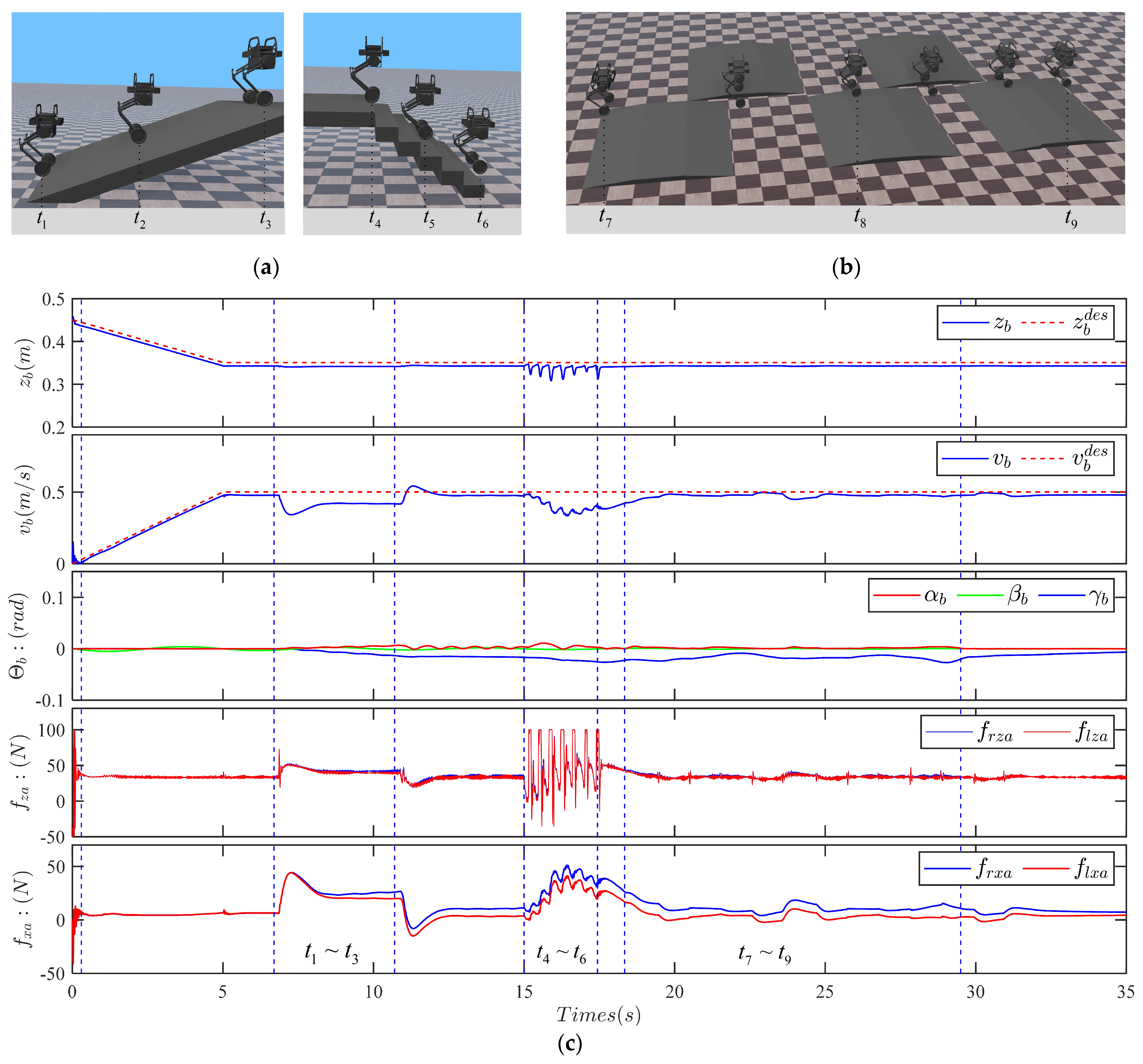
5.1. Going Uphill, Going Down Stairs and Crossing One-Sided Bridges

The uphill terrain is shown in Figure 8a, with a slope gradient of 0.348 rad and a length of 2 m. The down-stairs terrain is shown in Figure 8a, with a total elevation difference of 0.537 m and an elevation difference of 0.06 m between the steps. The terrain for crossing one-sided bridges is shown in Figure 8b, with up and down slopes of 0.1 rad and a maximum elevation difference of 0.1 m.

In the process of the controller design, it is necessary to design the torso position ${\left[\hspace{0.17em}{x}_b\hspace{1em}{z}_b\hspace{1em}\alpha \hspace{1em}\beta \hspace{1em}\gamma \hspace{1em}{v}_b\hspace{1em}{\dot{z}}_b\hspace{1em}\dot{\alpha }\hspace{1em}\dot{\beta }\hspace{1em}\dot{\gamma }\hspace{0.17em}\right]}^T$ weight values, and in the process of movement, the values of the wheeled-bipedal robot station height, forward velocity, traverse roll angle, pitch angle and yaw angle follow the principle of first large and then small, corresponding to the proportionality of the principle of the position weight matrix, Q, and the input weight matrix, R. The two sets of parameters selected are as follows:

$$\begin{array}{l}P1:\left\{\begin{array}{l}Q=diag\left[0,30000,10000,400,600, 2100,10,10,10,10\right]\\ R=diag\left[0.001,0.001,1,0.001,0.001,1\right]\end{array}\right.\\ P2:\left\{\begin{array}{l}Q=diag\left[0,300000,100000,4000,6000, 2100,10,10,10,10\right]\\ R=diag\left[0.001,0.001,1,0.001,0.001,1\right]\end{array}\right.\end{array}$$

(22)

Both sets of parameters can enable the wheeled-bipedal robot to complete the desired motion in the simulation experiments, as shown in Figure 9, but although the P1 parameter group can complete the desired motion, the maximum error of the robot’s standing height in the down-stairs stage is 0.07 m, and the static error of the robot’s standing height in the dynamic stabilization stage is 0.026 m. As a result of this, the weights of the standing height are increased and the rest of the weights are fine-tuned, and the maximum error of the robot’s standing height in the down-stairs stage is 0.04 m. The static error of the rest of the torso positions is 0.008 m, which is obviously better than that of the P1 parameter group. The maximum error of the robot’s station height in the down-stairs stage is 0.04 m, the static error of the robot’s station height in the dynamic stabilization stage is 0.008 m and the error value of the rest of the torso postures is significantly better than that of the P1 parameter group; thus, the P2 parameter group is chosen for all subsequent simulation experiments to control the wheeled-bipedal robot.

The desired speed of the robot’s torso during the passage through the above terrain is 0.5 $\mathrm{m}/{\mathrm{s}}^2$ acceleration during the 0–5 s period, followed by a uniform traveling speed. The desired standing height of Skater-I is as follows: the initial standing height for Skater-I is 0.451 m, and the rate of change in the standing height is maintained at −0.02 m/s during the 0–5 s period, after which the standing height remains constant. We set the desired values of the robot torso roll angle ${\alpha }_b$, pitch angle ${\beta }_b$ and yaw angle ${\gamma }_b$ to 0 rad.

The initial position wheel of the robot was 1 cm above the ground. Skater-I’s standing height $z_b$ and torso velocity $v_b$ fluctuated greatly at the beginning of the experiment and then stabilized after 0.3 s. The $t_1~t_3$ time period is the uphill phase of the robot, and the controller adaptively adjusts $f_{xa}$ to ensure that the torso velocity $v_b$ follows the accuracy of the desired torso velocity $v_b^{des}$. As shown in Figure 10c, the maximum error is 0.157 m/s, and the error in the stabilization phase is in the range of [0, 0.08] m/s as the force increases.

The $t_4~t_6$ time period is the down-stairs phase, as shown in Figure 10a, and Skater-I’s standing height $z_b$ and the active driving force of the wheeled legs on the torso $f_{za}$ undergo periodic fluctuations. As can be seen from Figure 10c, Skater-I’s standing height $z_b$ error is always within [0, 0.05] m and is in a stable state. When Skater-I is descending each section of the ladder, under the influence of gravity, Skater-I is unable to buffer in advance due to the absence of external sensors, and the downward force at the moment it touches the ground will be steeply increased, resulting in an abrupt change in Skater-I’s standing height $z_b$. And the active force solver will instantly increase the upward active force from the wheeled leg to the trunk to restore Skater-I’s standing height to the desired standing height, and the sequential cyclic change will occur. The forward velocity $v_b$ fluctuates because Skater-I is unable to adjust the forward velocity during the hovering phase and can only adjust the forward velocity when it touches the ground, which results in fluctuations in the velocity error, and at the same time, the horizontal force in the active force solver fluctuates following the fluctuations in the torso velocity $v_b$. Although the torso position of Skater-I fluctuates due to the terrain, the controller is not affected by the terrain and quickly stabilizes the position of Skater-I.

As shown in Figure 10b, the $t_7~t_9$ time period is the phase that involves crossing one-sided bridges. Skater-I’s standing height $z_b$ error is within the range of [0, 0.008] m when crossing different one-sided bridges. As shown in Figure 10c, the torso velocity errors are within [0, 0.05] m/s; the torso roll angle ${\alpha }_b$, pitch angle ${\beta }_b$ and yaw angle ${\gamma }_b$ errors are within [0, 0.027] rad and are at convergence.

During this simulation experiment, although the robot’s torso position fluctuates due to the influence of the terrain, the hierarchical control framework adjusts the active driving force of the wheeled legs on the torso so that Skater-I’s standing height $z_b$, torso velocity $v_b$, torso roll angle ${\alpha }_b$, torso pitch angle ${\beta }_b$ and torso yaw angle ${\gamma }_b$ are kept within the permissible error range and follow the desired values effectively. This simulation experiment demonstrates the effectiveness of the hierarchical control framework in controlling the posture of the torso.

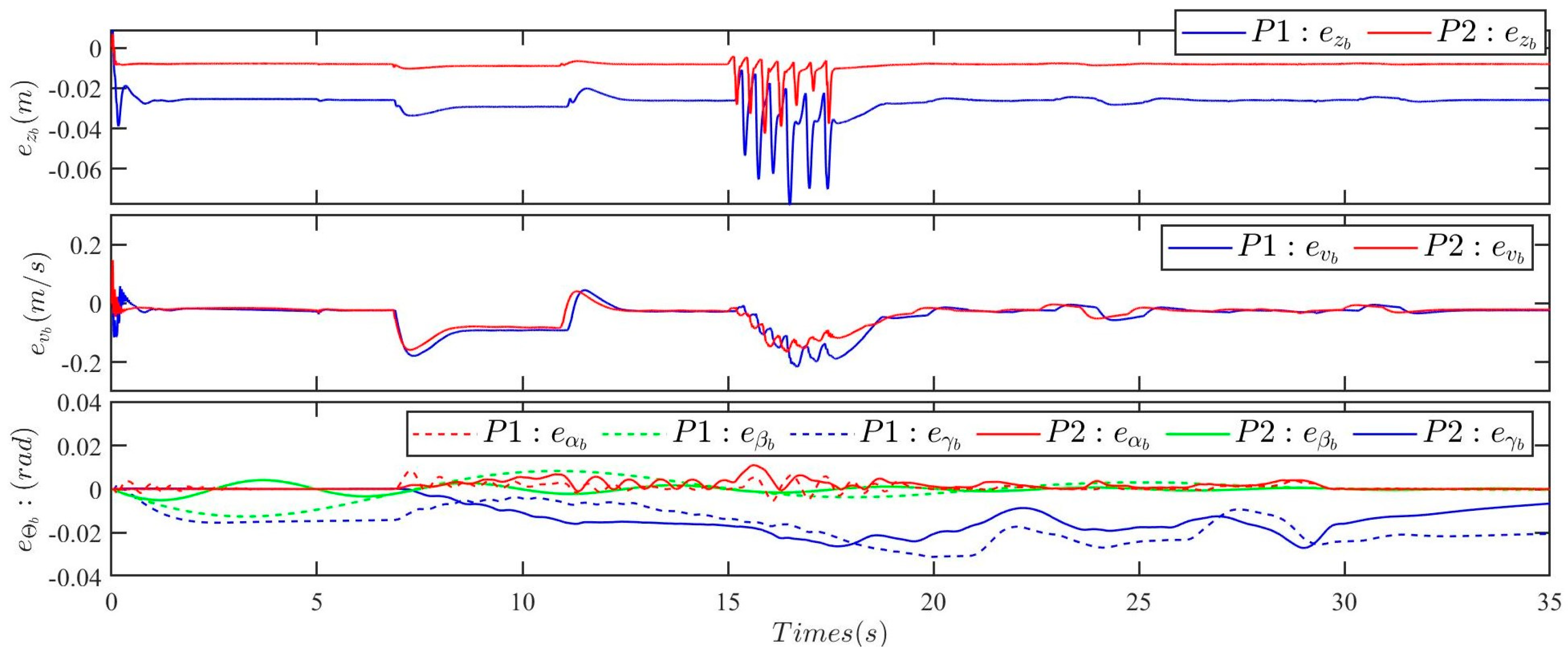
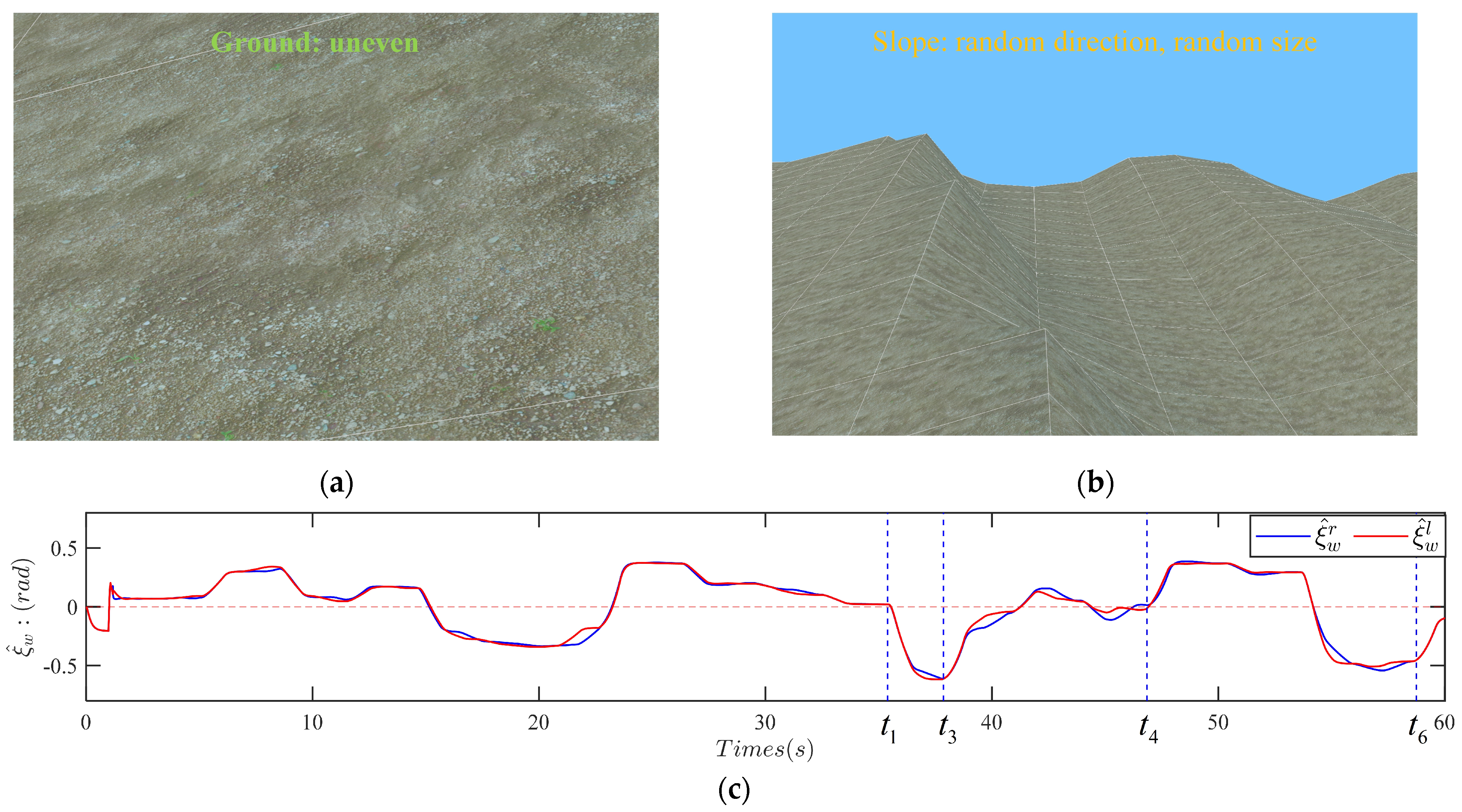
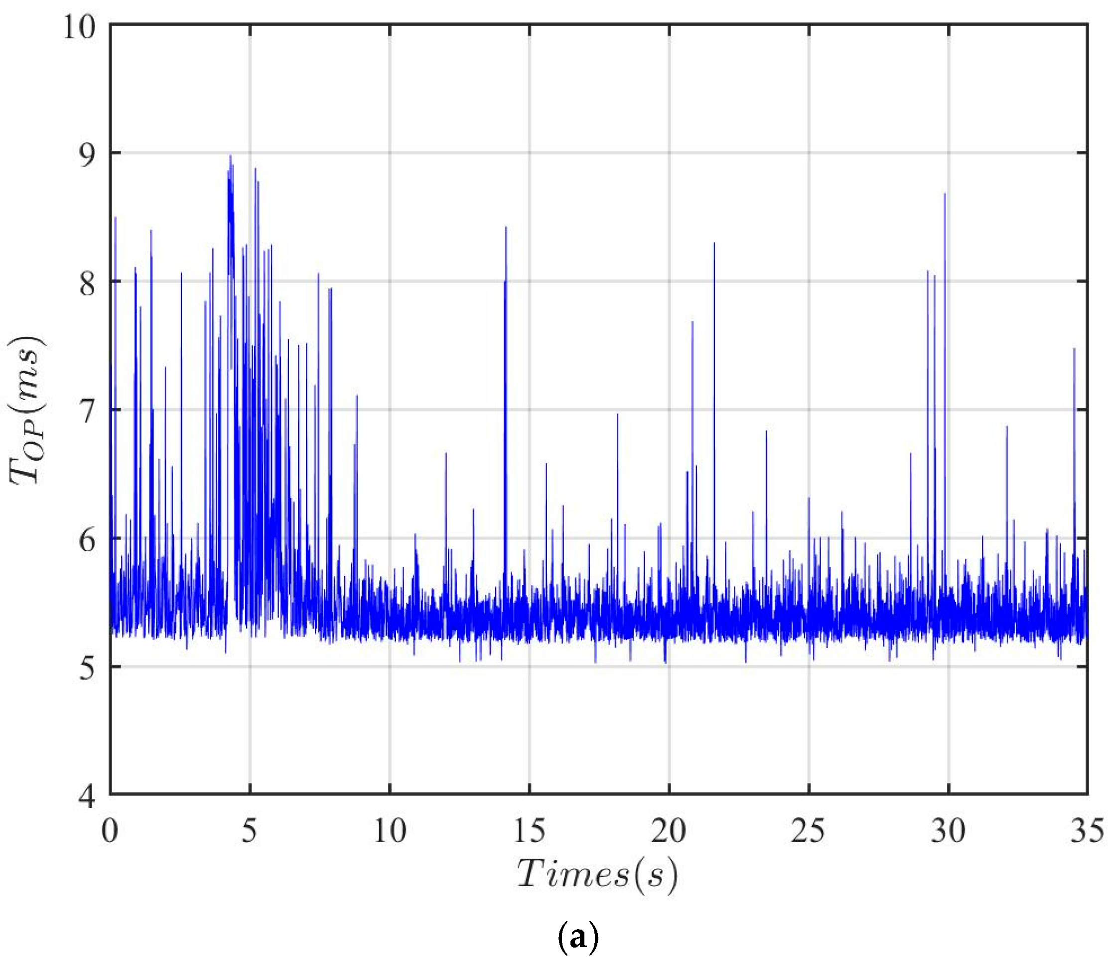
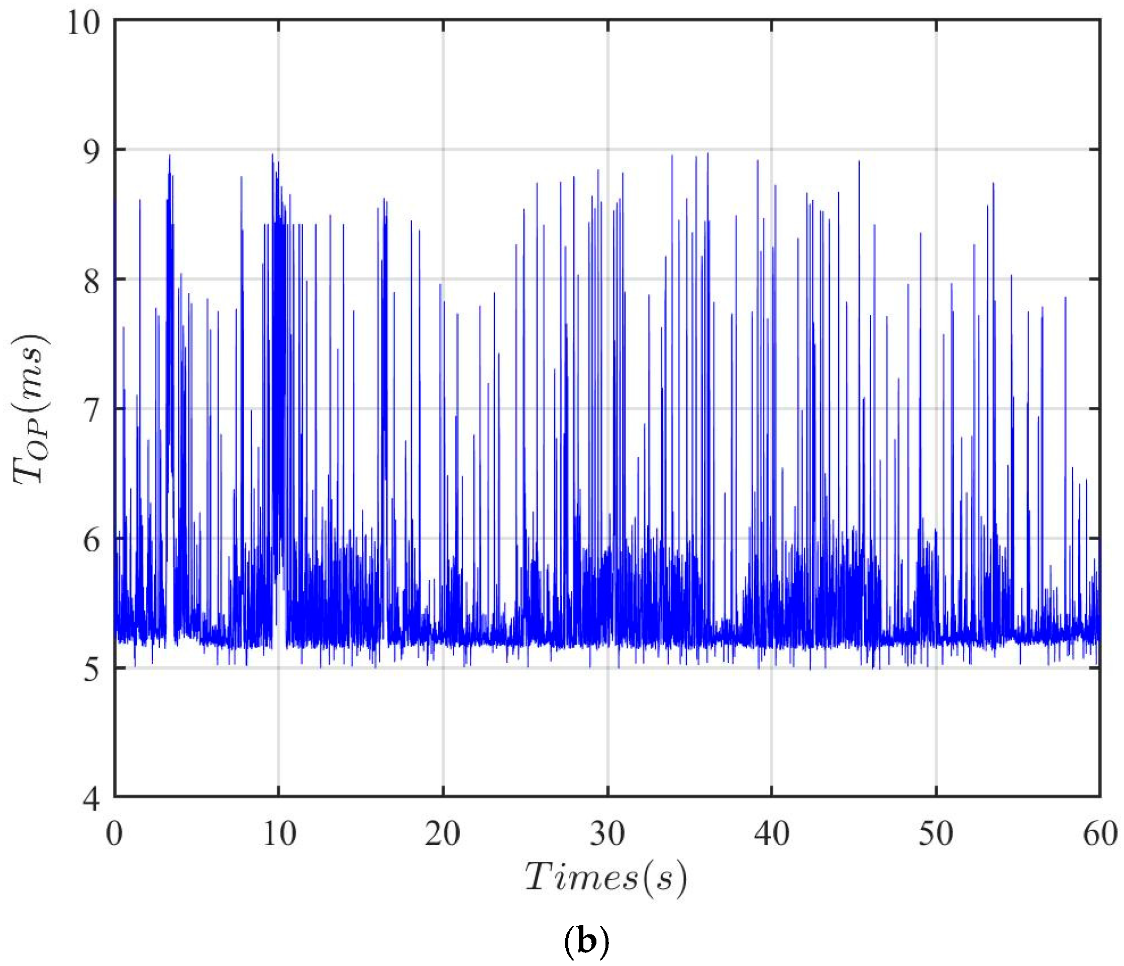
5.2. Simulation Experiments on Uneven Terrain

The uneven terrain is shown in Figure 11a,b. The slope of the uneven terrain mentioned in the simulation experiments is continuously changing, not only in terms of the longitudinal slope but also the transverse slope, and the distribution of the longitudinal and transverse slopes is random in which the ground surface is also irregular and uneven. The longitudinal slope angle is estimated in real time using Equation (16), and the results are shown in Figure 11c, which shows that the traveling slope angles of the left wheeled leg and the right wheeled leg are basically the same, and the slope estimation value ${\widehat{\xi }}_w$ is in the range of [−0.612, 0.387] rad.

During the robot’s motion, the $t_1~t_3$ phase is a downhill section, where the average slope is −0.5 rad, as shown in Figure 12a. During the descent, $f_{xa}$ and $f_{za}$ decrease, and as shown in Figure 12b, Skater-I’s standing height $z_b$ error remains within [0, 0.005] m, and the torso velocity $v_b$ error remains within [0, 0.14 ] m/s. The ${\mathrm{\alpha }}_b$, ${\mathrm{\beta }}_b$ and ${\mathrm{\gamma }}_b$ errors all remain within [0, 0.012] rad and stabilize quickly.

Phase $t_4~t_6$ is an uphill and then downhill section, where the average gradient is 0.3 rad for the uphill experiment and 0.5 rad for the downhill experiment, as shown in Figure 12a. $f_{xa}$ and $f_{za}$ increase when going uphill and decrease when going downhill, as shown in Figure 12b, and Skater-I’s standing height $z_b$ error is kept in the range of [0.005, 0.009] m, while the torso velocity $v_b$ error is kept in the range of [0, 0.16] m/s. The ${\mathrm{\alpha }}_b$, ${\mathrm{\beta }}_b$ and ${\mathrm{\gamma }}_b$ errors are maintained within [0, 0.06] rad and stabilize quickly. Skater-I’s standing height, and the velocity, roll angle, pitch angle and yaw angle of the robot’s torso converge rapidly after being affected by the unstructured terrain and remain to follow the desired state, which fully demonstrates the robustness as well as the anti-jamming property of the hierarchical control framework.

To analyze how Skater-I maintains its stability in different terrains, the wheeled leg attitude $\varphi$ of Skater-I is defined as shown in Equation (23):

$$\varphi ={\displaystyle \frac{△x}{z_n}}$$

(23)

where $△x$ denotes the vertical distance at the point of contact between the hip joint and the wheel ground, and $z_n$ denotes the horizontal distance at the point of contact between the hip joint and the wheel ground. During Skater-I’s motion, the wheeled leg’s balance attitude ${\varphi }_b$ is as shown in Equation (24):

$${\varphi }_b={\displaystyle \frac{a_b^d}{g}}$$

(24)

where $a_b^d$ denotes the expected horizontal acceleration of the torso and $g$ denotes the gravitational acceleration. Skater-I reaches dynamic equilibrium when the robot’s wheeled leg attitude $\varphi$ is equal to the balanced wheeled leg attitude ${\varphi }_b$. Skater-I experiments going uphill, down stairs, crossing one-sided bridges and traveling on uneven terrain. Skater-I will be affected by the terrain change, for example, when the terrain slope suddenly increases, and Skater-I’s wheel–ground contact point is shifted forward, resulting in the current wheeled leg stance being smaller than the wheeled leg equilibrium stance, and it is out of the dynamic equilibrium state. With the station height kept constant, the active horizontal virtual force output from the wheeled leg subsystem is reduced, resulting in the actual acceleration of the torso being less than the desired acceleration of the torso. At this time, the horizontal active force solved by the active force solver becomes larger, and the $△x$ value also becomes larger, so the wheeled leg attitude is gradually adjusted to the balanced wheeled leg attitude, which completes the automatic adjustment of the wheeled leg attitude and brings Skater-I into a new dynamic equilibrium.

The TIMESTEP of Skater-I is designed to be 10 ms during the movement of Skater-I. During the simulation experiments going uphill, down stairs, crossing one-sided bridges and the simulation experiments on uneven terrain, the hardware and the device parameters are cpu: Intel(R) Core(TM) i5-10210U CPU @1.60 GHz; RAM: 16.0 GB; GPU: NVIDIA GeForce MX250 and Webots software version: Webots R2021a. Additionally, we define the time required for controller computation under the step length of Skater-I as $T_{OP}$. As shown in Figure 13, the controller computation times in the simulation experiments are all less than 10 ms. The average value of $T_{OP}$ is 5.47 ms in the experiments involving going uphill, going down stairs and crossing one-sided bridges, and the average value of $T_{OP}$ is 5.53 ms in the simulation experiments on uneven terrain. In the simulation experiments on uneven terrain, the average value of $T_{OP}$ is 5.53 ms, which is less than the TIMESTEP of Skater-I and meets the design requirements; thus, real-time control can be achieved in the movement of Skater-I.

6. Conclusions

In this paper, the modeling and control methods for WBRs are explored in detail. Based on the distributed dynamics modeling method, a whole-body control method is proposed. The active force of the wheeled leg system on the torso system is calculated by an active force distributor based on model predictive control, and a whole-body attitude planner is utilized to enhance the adaptability of the WBRs on uneven terrain, combining the active force distributor and the whole-body attitude planner to resolve the desired motion of the robot’s torso into the articulation torques of the wheeled leg joints. Skater-I performs tasks of passing through a terrain while going up a slope, descending a staircase and crossing one-sided bridges with maximum errors of 9 mm for the torso. The maximum errors of the torso height following and torso velocity following are 8 mm and 0.05 m/s, respectively; the maximum error of the roll angle following, pitch angle following and yaw angle following is 0.02 rad; and the errors of the above-mentioned parameters are kept within the permissible error range and converge quickly. The maximum errors of the torso height following and torso speed following are 9 mm and 0.16 m/s, respectively, and the maximum error of the traverse angle following, pitch angle following and yaw angle following is 0.06 rad. The errors of the above parameters are kept within the permissible error range and converge. Through simulation experiments and an experimental data analysis, it is proven that the WBR Skater-I under whole-body control can adapt to uneven terrain and shows high stability in motion on uneven terrain.

In the future, physical experiments will be conducted using the research presented in this paper to further validate the effectiveness and stability of whole-body control with the uneven terrain adaptability strategy in Skater-I. Subsequent planning and control of various movement modes, such as jumping and wheeled skating, will be conducted to further improve the ability of Skater-I to pass through uneven terrain in complex environments.

References

1. Hougen, D.F.; Benjaafar, S.; Bonney, J.C.; Budenske, J.R.; Dvorak, M.; Gini, M.; French, H.; Krantz, D.G.; Li, P.Y.; Malver, F.; et al. A miniature robotic system for reconnaissance and surveillance. In Proceedings of the 2000 ICRA. Millennium Conference. IEEE International Conference on Robotics and Automation. Symposia Proceedings (Cat. No. 00CH37065), San Francisco, CA, USA, 24–28 April 2000; IEEE: New York, NY, USA, 2000; Volume 1, pp. 501–507. [Google Scholar] [CrossRef]
2. Pedro, G.D.G.; Bermudez, G.; Medeiros, V.S.; Cruz Neto, H.J.d.; Barros, L.G.D.d.; Pessin, G.; Becker, M.; Freitas, G.M.; Boaventura, T. Quadruped Robot Control: An Approach Using Body Planar Motion Control, Legs Impedance Control and Bézier Curves. Sensors 2024, 24, 3825. [Google Scholar] [CrossRef] [PubMed]
3. Bruzzone, L.; Quaglia, G. Locomotion systems for ground mobile robots in unstructured environments. Mech. Sci. 2012, 3, 49–62. [Google Scholar] [CrossRef]
4. Liu, T.; Zhang, C.; Song, S.; Meng, M.Q.H. Dynamic height balance control for bipedal wheeled robot based on ROS-Gazebo. In Proceedings of the 2019 IEEE International Conference on Robotics and Biomimetics (ROBIO), Dali, China, 6–8 December 2019; IEEE: New York, NY, USA, 2019; pp. 1875–1880. [Google Scholar] [CrossRef]
5. Bellicoso, C.D.; Jenelten, F.; Fankhauser, P.; Gehring, C.; Hwangbo, J.; Hutter, M. Dynamic locomotion and whole-body control for quadrupedal robots. In Proceedings of the 2017 IEEE/RSJ International Conference on Intelligent Robots and Systems (IROS), Vancouver, BC, Canada, 24–28 September 2017; IEEE: New York, NY, USA, 2017; pp. 3359–3365. [Google Scholar] [CrossRef]
6. Liu, X.; Yang, L.; Chen, Z.; Zhong, J.; Gao, F. Motion Planning for a Legged Robot with Dynamic Characteristics. Sensors 2024, 24, 6070. [Google Scholar] [CrossRef] [PubMed]
7. Fahmi, S.; Mastalli, C.; Focchi, M.; Semini, C. Passive whole-body control for quadruped robots: Experimental validation over challenging terrain. IEEE Robot. Autom. Lett. 2019, 4, 2553–2560. [Google Scholar] [CrossRef]
8. Chen, T.; Sun, X.; Xu, Z.; Li, Y.; Rong, X.; Zhou, L. A trot and flying trot control method for quadruped robot based on optimal foot force distribution. J. Bionic Eng. 2019, 16, 621–632. [Google Scholar] [CrossRef]
9. Faigl, J.; Čížek, P. Adaptive locomotion control of hexapod walking robot for traversing rough terrains with position feedback only. Robot. Auton. Syst. 2019, 116, 136–147. [Google Scholar] [CrossRef]
10. Khadiv, M.; Herzog, A.; Moosavian, S.A.A.; Righetti, L. Walking control based on step timing adaptation. IEEE Trans. Robot. 2020, 36, 629–643. [Google Scholar] [CrossRef]
11. Hutter, M.; Sommer, H.; Gehring, C.; Hoepflinger, M.; Bloesch, M.; Siegwart, R. Quadrupedal locomotion using hierarchical operational space control. Int. J. Robot. Res. 2014, 33, 1047–1062. [Google Scholar] [CrossRef]
12. Stilman, M.; Wang, J.; Teeyapan, K.; Marceau, R. Optimized control strategies for wheeled humanoids and mobile manipulators. In Proceedings of the 2009 9th IEEE-RAS International Conference on Humanoid Robots, Paris, France, 7–10 December 2009; IEEE: New York, NY, USA, 2009; pp. 568–573. [Google Scholar] [CrossRef]
13. Zhao, L.; Yu, Z.; Han, L.; Chen, X.; Qiu, X.; Huang, Q. Compliant Motion Control of Wheel-Legged Humanoid Robot on Rough Terrains. IEEE/ASME Trans. Mechatron. 2023, 29, 1949–1959. [Google Scholar] [CrossRef]
14. Li, X.; Fu, Y. Design and Experimental Evaluation of WLR-III. In Proceedings of the 2023 IEEE International Conference on Robotics and Biomimetics (ROBIO), Koh Samui, Thailand, 4–9 December 2023; IEEE: New York, NY, USA, 2023; pp. 1–6. [Google Scholar] [CrossRef]
15. Li, X.; Zhang, S.; Zhou, H.; Feng, H.; Fu, Y. Locomotion adaption for hydraulic humanoid wheel-legged robots over rough terrains. Int. J. Humanoid Robot. 2021, 18, 2150001. [Google Scholar] [CrossRef]
16. Zhou, H.; Li, X.; Feng, H.; Li, J.; Zhang, S.; Fu, Y. Model decoupling and control of the wheeled humanoid robot moving in sagittal plane. In Proceedings of the 2019 IEEE-RAS 19th International Conference on Humanoid Robots (Humanoids), Toronto, ON, Canada, 15–17 October 2019; IEEE: New York, NY, USA, 2019; pp. 1–6. [Google Scholar] [CrossRef]
17. Li, X.; Zhou, H.; Zhang, S.; Feng, H.; Fu, Y. WLR-II, a hose-less hydraulic wheel-legged robot. In Proceedings of the 2019 IEEE/RSJ International Conference on Intelligent Robots and Systems (IROS), Macau, China, 3–8 November 2019; IEEE: New York, NY, USA, 2019; pp. 4339–4346. [Google Scholar] [CrossRef]
18. Li, X.; Zhou, H.; Feng, H.; Zhang, S.; Fu, Y. Design and experiments of a novel hydraulic wheel-legged robot (WLR). In Proceedings of the 2018 IEEE/RSJ International Conference on Intelligent Robots and Systems (IROS), Madrid, Spain, 1–5 October 2018; IEEE: New York, NY, USA, 2018; pp. 3292–3297. [Google Scholar] [CrossRef]
19. Klemm, V.; Morra, A.; Salzmann, C.; Tschopp, F.; Bodie, K.; Gulich, L.; Küng, N.; Mannhart, D.; Pfister, C.; Vierneisel, M.; et al. Ascento: A two-wheeled jumping robot. In Proceedings of the 2019 International Conference on Robotics and Automation (ICRA), Montreal, QC, Canada, 20–24 May 2019; IEEE: New York, NY, USA, 2019; pp. 7515–7521. [Google Scholar] [CrossRef]
20. Klemm, V.; Morra, A.; Gulich, L.; Mannhart, D.; Rohr, D.; Kamel, M.; de Viragh, Y.; Siegwart, R. LQR-assisted whole-body control of a wheeled bipedal robot with kinematic loops. IEEE Robot. Autom. Lett. 2020, 5, 3745–3752. [Google Scholar] [CrossRef]
21. Xin, S.; Vijayakumar, S. Online dynamic motion planning and control for wheeled biped robots. In Proceedings of the 2020 IEEE/RSJ International Conference on Intelligent Robots and Systems (IROS), Las Vegas, NV, USA, 24 October 2020–24 January 2021; IEEE: New York, NY, USA, 2020; pp. 3892–3899. [Google Scholar] [CrossRef]
22. Cao, H.; Lu, B.; Liu, H.; Liu, R.; Guo, X. Modeling and MPC-based balance control for a wheeled bipedal robot. In Proceedings of the 2022 41st Chinese Control Conference (CCC), Hefei, China, 25–27 July 2022; IEEE: New York, NY, USA, 2022; pp. 420–425. [Google Scholar] [CrossRef]
23. Zhang, J.; Wang, S.; Wang, H.; Lai, J.; Bing, Z.; Jiang, Y.; Zheng, Y.; Zhang, Z. An adaptive approach to whole-body balance control of wheel-bipedal robot Ollie. In Proceedings of the 2022 IEEE/RSJ International Conference on Intelligent Robots and Systems (IROS), Kyoto, Japan, 23–27 October 2022; IEEE: New York, NY, USA, 2022; pp. 12835–12842. [Google Scholar] [CrossRef]
24. Chen, Z.; Zhan, G.; Jiang, Z.; Zhang, W.; Rao, Z.; Wang, H.; Li, J. Adaptive impedance control for docking robot via Stewart parallel mechanism. ISA Trans. 2024, 155, 361–372. [Google Scholar] [CrossRef] [PubMed]
25. Xu, Y.; Chen, Z.; Deng, C.; Wang, S.; Wang, J. LCDL: Towards Dynamic Localization for Autonomous Landing of Unmanned Aerial Vehicle Based on LiDAR-Camera Fusion. IEEE Sens. J. 2024, 24, 26407–26415. [Google Scholar] [CrossRef]
26. Abbasimoshaei, A.; Stein, T.; Rothe, T.; Kern, T.A. Design and impedance control of a hydraulic robot for paralyzed people. In Proceedings of the 8th RSI International Conference on Robotics and Mechatronics, ICRoM 2020, Virtual, Online, 19 November 2020. [Google Scholar]
27. Wei, Z.; Deng, W.; Feng, Z.; Wang, T.; Huang, X. An MPC-DCM Control Method for a Forward-Bending Biped Robot Based on Force and Moment Control. Electronics 2024, 13, 4374. [Google Scholar] [CrossRef]
28. Xu, J.; Zhao, M.; Zhang, T.; Ji, A. A Rigid–Flexible Supernumerary Robotic Arm/Leg: Design, Modeling, and Control. Electronics 2024, 13, 4106. [Google Scholar] [CrossRef]
29. Xin, Y.; Chai, H.; Li, Y.; Rong, X.; Li, B.; Li, Y. Speed and acceleration control for a two wheel-leg robot based on distributed dynamic model and whole-body control. IEEE Access 2019, 7, 180630–180639. [Google Scholar] [CrossRef]
30. Xin, Y.; Rong, X.; Li, Y.; Li, B.; Chai, H. Movements and balance control of a wheel-leg robot based on uncertainty and disturbance estimation method. IEEE Access 2019, 7, 133265–133273. [Google Scholar] [CrossRef]
31. Wang, Y.; Chen, T.; Rong, X.; Zhang, G.; Li, Y.; Xin, Y. Design and Control of SKATER: A Wheeled-Bipedal Robot With High-Speed Turning Robustness and Terrain Adaptability. IEEE/ASME Trans. Mechatron. 2024, 1–12. [Google Scholar] [CrossRef]
Figure 1. Schematic diagram of Skater-I robot.
Electronics 14 00198 g001
Figure 2. Diagram of coordinate system position relationship.
Electronics 14 00198 g002
Figure 3. Skater-I robot’s force transfer relationship between wheeled legs and torso.
Electronics 14 00198 g003
Figure 4. A schematic of the WBR torso coordinate system, active force and positional attitude.
Electronics 14 00198 g004
Figure 5. The setup of the unilateral wheeled-legged coordinate system with the wheel as the moving base.
Electronics 14 00198 g005
Figure 6. A hierarchical control framework diagram. τ f f is the torque solved from the inverse dynamics of the wheeled leg, P b are the coordinates of the wheel–ground contact point in the coordinate system b and p ˙ b is the velocity of the wheel–ground contact point in the coordinate system b .
Electronics 14 00198 g006
Figure 7. Schematic of robot roll angle on uneven terrain.
Electronics 14 00198 g007
Figure 8. Schematic diagram of simulated terrains: (a) schematic of uphill and down-stairs terrains; (b) schematic of terrain with one-sided bridges.
Electronics 14 00198 g008
Figure 9. Comparison of torso position errors of wheeled-bipedal robot corresponding to two different sets of parameters.
Electronics 14 00198 g009
Figure 10. Experiments of going uphill and downhill and crossing one-sided bridges. (a) Snapshots of postures when going uphill and down stairs. (b) Snapshot of crossing one-sided bridges. (c) robot status and active driving force, where z b is Skater-I’s standing height, v b is the torso velocity and Θ b includes the torso roll angle α b , torso pitch angle β b and torso yaw angle γ b . f x a and f z a are the horizontal active driving force and longitudinal active driving force provided by the wheeled leg system to the torso system.
Electronics 14 00198 g010
Figure 11. Overview of uneven terrain. (a) Schematic of unstructured terrain ground. (b) Schematic of unstructured terrain slope. (c) Estimated slope angles, where ξ ^ w r and ξ ^ w l are estimated terrain slopes for left and right wheeled legs, respectively.
Electronics 14 00198 g011
Figure 12. Unstructured terrain simulation experiment: (a) a snapshot of the t 1 ~ t 3 phase and t 4 ~ t 6 phase; (b) the robot’s status and active driving force, where z b is Skater-I’s standing height, v b is the torso velocity, and Θ b includes the torso roll angle α b , pitch angle β b and yaw angle γ b . f x a and f z a are the virtual horizontal and longitudinal forces provided by the wheeled leg system to the torso system.
Electronics 14 00198 g012
Figure 13. Schematic representation of time required for controller computation T O P under step size for Skater-I. (a) Schematic of T O P in experiments involving going uphill and down stairs and crossing one-sided bridges. (b) Schematic representation of T O P in simulation experiments on uneven terrain.
Electronics 14 00198 g013aElectronics 14 00198 g013b