Dung Beetle Optimization Algorithm Based on Improved Multi-Strategy Fusion

Abstract

The Dung Beetle Optimization Algorithm (DBO) is characterized by its great convergence accuracy and quick convergence speed. However, like other swarm intelligent optimization algorithms, it also has the disadvantages of having an unbalanced ability to explore the world and to use local resources, as well as being prone to settling into local optimal search in the latter stages of optimization. In order to address these issues, this research suggests a multi-strategy fusion dung beetle optimization method (MSFDBO). To enhance the quality of the first solution, the refractive reverse learning technique expands the algorithm search space in the first stage. The algorithm’s accuracy is increased by adding an adaptive curve to control the dung beetle population size and prevent it from reaching a local optimum. In order to improve and balance local exploitation and global exploration, respectively, a triangle wandering strategy and a fusion subtractive averaging optimizer were later added to Rolling Dung Beetle and Breeding Dung Beetle. Individual beetles will congregate at the current optimal position, which is near the optimal value, during the last optimization stage of the MSFDBO; however, the current optimal value could not be the global optimal value. Thus, to variationally perturb the global optimal solution (so that it leaps out of the local optimal solution in the final optimization stage of the MSFDBO) and to enhance algorithmic performance (generally and specifically, in the effect of optimizing the search), an adaptive Gaussian–Cauchy hybrid variational perturbation factor is introduced. Using the CEC2017 benchmark function, the MSFDBO’s performance is verified by comparing it to seven different intelligence optimization algorithms. The MSFDBO ranks first in terms of average performance. The MSFDBO can lower the labor and production expenses associated with welding beam and reducer design after testing two engineering application challenges. When it comes to lowering manufacturing costs and overall weight, the MSFDBO outperforms other swarm intelligence optimization methods.

1. Introduction

The rapid expansion of the economy and society has long led to a number of optimization challenges in various industries. An optimization problem is to find the optimal solution or parameter among multiple solutions or parameter values by means of constraints in order to optimize one or more functions. At the same time, optimization problems involve a wide range of applications, such as path planning [1], feature selection [2], image processing [3], mechanical design [4], neural network parameter optimization [5], etc., and the core of such problems is to select the optimal solution to maximize the benefit of the objective. In practice, the difficulty and complexity of engineering optimization problems in various fields are increasing, which increase the need for efficient algorithms. Researchers have, therefore, created a variety of swarm intelligence optimization algorithms, which can more swiftly tackle intricate and varied problems by examining the actions of the creatures. Numerous sophisticated and challenging optimization issues have been solved using these strategies.

In recent years, many publications on swarm intelligence optimization algorithms have been released, including PSO [6], GWO [7], WOA [8], HHO [9], SSA [10], SSA [11], DBO [12], SCSO [13], SO [14], GJO [15], and others. They are used in various fields with good results. Many academics have enhanced the initial swarm intelligence optimization algorithms for handling more complicated real-world applications as the “No Free Lunch Theorem” [16] states that no single swarm intelligence optimization algorithm can solve all optimization problems. For example, an enhanced dung beetle optimization algorithm based on quantum computation and multi-strategy was presented by Fang Zhu et al. [17]. Given a set of starting points, the population of dung beetles was dynamically balanced between egg-laying and foraging individuals. The globally optimal solution was variationally perturbed, using a t-distribution variational technique based on quantum computation, to prevent the program from reaching a local optimum. The enhanced algorithm’s better performance was shown using 37 test functions and engineering. To balance exploration and exploitation, Yuchen Duan et al. [18] fused the SCA to the GWO. They performed this by using the CEC2013, 2014, and 2019 test functions to demonstrate that the improved pronouncements have a faster convergence rate and better convergence accuracy. Saroj Kumar Sahoo et al. [19] proposed an improved dynamic dyadic learning moth-based optimization algorithm and applied the improved dynamic dyadic learning strategy to the moth optimization algorithm, comparing it with a series of optimization algorithms on the CEC2014 so as to verify that the improved algorithm has good performance. In order to address the shortcomings of the sparrow optimization algorithm in terms of low individual utilization and lack of effective search, Shaoqiang Yan et al. [20] introduced variable spiral factors and an improved local search strategy in the global and local phases of the follower’s search, respectively, to increase its search capability, and used a dimension-by-dimension lens learning strategy to help it jump out of the local optimal solution. Qi Yao et al. [21] proposed IDBO, which is based on Fuch chaotic mapping and a convex lens inverse imaging strategy, and used IDBO to perform hyper-parameter optimization of BiLSTM for better application to related practical problems. Yinggao Yue et al. [22] proposed SCAGTO, which combines the Cauchy distribution and sine–cosine strategies. The population is initialized using a refractive inverse learning mechanism, and the algorithm introduces a sine–cosine strategy at the search position and a Cauchy distribution in order to cause the population to deviate from the local optimum. Lastly, the algorithm’s superior optimization capability is verified through two engineering application problems and the engineering practicality of the algorithm. Through a comparative analysis with the remaining 10 algorithms on 20 benchmark datasets, Ahmed A. Ewees et al. [23] used the ISOA for feature selection, which eliminated the local optimum position by using the Lévy flight strategy and balance the explored and exploited performances by using mutation operators. It was shown that the ISOA has a high accuracy in feature selection, a low degree of adaptability, and the ability to select fewer individuals, as well as other indicators of superior performance compared to other algorithms. Yin Zhang et al. [24] proposed the LeNN-WOA-NM algorithm, which was based on the general approximation ability of the Ledgender neural network, which, in turn, used Legendre polynomials, and was supplemented by the WOA and Nelder Mead (NM) algorithms, for solving the numerical solution of TONMS-EFE. The superior performance of LeNN WOA-NM in solving TONMS-EFE was verified by comparing it with the PSO and Cuckoo search algorithm (CSA). Based on partitioned linear chaos mapping (PWLCM) and the dimensional learning augmented foraging strategy (DLF), Yujie Zhu et al. [25] proposed IDBO. Using the IDBO algorithm, the authors optimized the BP neural network’s parameters and thresholds and applied it to the corresponding real-world problems. The results of the experiments demonstrated that the IDBO-BP model has the smallest error and has advantages when processing real-world problems. In order to address the issue of becoming trapped in local optima, the aforementioned researchers have employed a variety of techniques to enhance swarm intelligent optimization algorithms. They still occasionally run into local optima, though, and are unable to locate the ideal spots. The MSFDBO algorithm is suggested as a solution to the issue of falling into local optima, in light of the aforementioned concerns.

DBO features a quick rate of convergence and a significant capacity for optimization seeking. In the meantime, DBO has been successfully applied to several engineering design optimization problems by the authors of the original paper, and the experimental findings demonstrate that it can handle real-world issues. Nevertheless, DBO is also hampered by its inadequate global exploration capability, a propensity to enter local optima, and an imbalance between global exploration and local exploitation skills. Consequently, the MSFDBO is proposed in this study. The following are this study’s primary contributions:

Firstly, a multi-strategy fusion dung beetle optimization algorithm (MSFDBO) is proposed. The MSFDBO introduces the following improvements to the basic DBO:

(1)

To increase the search space of the algorithm, a refractive backward learning method is employed, and an adaptive curve is included to control the size of the dung beetle population.

(2)

To enhance and balance local exploitation and global exploration, the algorithm’s convergence is accelerated in the ball-rolling dung beetle phase by using a triangular wandering approach and in the breeding dung beetle phase by using a fused subtractive averaging optimizer.

(3)

Late in the iteration, the globally optimal solution is variationally disturbed by an adaptive Gaussian–Cauchy hybrid variational perturbation factor, which improves algorithm efficiency and the impact of finding the ideal solution.

Secondly, under 29 benchmark test functions, the MSFDBO’s efficacy was confirmed by comparison with seven original intelligence optimization algorithms.

Lastly, the experimental findings show that when the MSFDBO is used to solve two actual engineering application problems, it yields good test results.

The following is the structure of the paper: The DBO is described in Section 2. Section 3 provides a detailed description of the proposed MSFDBO algorithm, which includes the enhanced triangular wandering approach, adaptive curves, a fused subtractive averaging optimizer, and refractive backward learning procedures. The results of the Wilcoxon rank sum test and the CEC2017 benchmark test function are then used in Section 4 to evaluate the MSFDBO’s performance. Section 5 uses two engineering design issues to test the MSFDBO’s performance. In Section 6, the entire paper is summarized once more.

2. Dung Beetle Optimization Algorithm (DBO)

The DBO classifies beetles into four subpopulations, rolling, breeding, foraging, and stealing groups, with a strong optimality-seeking ability and fast convergence. The DBO model is described below.

2.1. Rolling Dung Beetle

Because light intensity affects the travel of a dung beetle and the sun is required for it to continue rolling a dung ball along a straight path in the absence of obstacles, the position update model is displayed below:

$$X_i(m+1)=X_i(m)+\omega \times k\times X_i(m-1)+b\times \Delta X$$

(1)

$$\Delta X=\left|X_i(m)-X^{worst}\right|$$

(2)

where $X_i(m)$ indicates the position data of the $i$ dung beetles at the $m\mathrm{th}$ iteration, $m$ indicates the current number of iterations, $\omega$ is a natural coefficient, given a value of 1 or −1, $\Delta X$ is the change in light intensity, $b$ denotes a constant in the range $(0,1)$, $X^{wrost}$ is the global worst position, and $k\in \left(0,0.2\right]$ indicates the constant of the deflection coefficient.

A dung beetle must dance to acquire a new rolling direction when it comes across an obstruction that prevents it from moving forward. Thus, the dung beetle’s mathematical model for figuring out its new rolling direction by dancing can be written as follows:

$$X_i(m+1)=X_i(m)+\tan (\theta )\left|X_i(m)-X_i(m-1)\right|$$

(3)

where $\theta \in \left[0,\pi \right]$, but will not change the dung beetle’s location when $\theta$ is equal to $0$, $\pi /2$ or $\pi$.

2.2. Breeding Dung Beetles

The dung beetle will select an appropriate location to lay its eggs after rolling the dung ball to a secure location once more. In order to model the region where female dung beetles lay their eggs, the original research suggests the following boundary selection strategy:

$$\begin{array}{l}L{b}^{\ast }=\max \left(X^{\ast }\times (1-R),Lb\right)\\ U{b}^{\ast }=\min \left(X^{\ast }\times (1-R),Ub\right)\end{array}$$

(4)

where $M$ indicates the current maximum number of iterations, $lb$ and $ub$ indicate the upper and lower bounds of the spawning area, respectively, $X_i^b$ indicates the current locally optimal position, $Q=1-m/M$, and $S_l$ and $S_u$ indicate the lower and higher borders, respectively.

The female dung beetle will select a spawning location after one has been identified. Each female dung beetle will only lay one egg due to the nature of its life cycle. Equation (4) shows that the spawning area’s boundary range is dynamically changing, primarily due to the Q value. Consequently, in the iterative process, the breeding dung beetle’s location is similarly dynamic and can be expressed as follows:

$$B_i(t+1)=X^{\ast }+b_1\times (B_i(t)-L{b}^{\ast })+b_2\times \left(B_i(t)-U{b}^{\ast }\right)$$

(5)

where ${\rho }_1$ and ${\rho }_2$ represent two independent random vectors $1\times D$, $D$ is the dimensionality of the optimization problem, and $X_i(m)$ is the location information of the $m\mathrm{th}$ breeding dung beetle at the $m\mathrm{th}$ iteration.

2.3. Foraging Dung Beetles

The best foraging location must be determined once the juvenile dung beetles hatch to direct them to food in a manner that mimics their natural foraging behavior. The ideal foraging area’s limits are specifically established as follows:

$$\begin{array}{l}{K}_l=\max \left(X^b\times (1-Q),lb\right)\\ K_u=\min (X^b\times (1-Q),ub)\end{array}$$

(6)

where $K_l$ and $K_u$ represent the bottom and upper bounds of the optimal foraging area, respectively, and $X^b$ represents the global best position. The following formula is used to update the little dung beetle’s position after identifying the optimal foraging area:

$$X_i(m+1)=X_i(m)+{\beta }_1\times (X_i(m)-K_l)+{\beta }_2\times (X_i(m)-K_u)$$

(7)

where ${\beta }_1$ is a random integer that follows a normal distribution, ${\beta }_2$ is the quantity of random variable that falls between 0 and 1, and $X_i(m)$ is the position information of the $i\mathrm{th}$ small dung beetle at the C iteration.

2.4. Stealing Dung Beetles

Certain dung beetles are referred to as thieves because they feed on the feces of other dung beetles. Equation (6) indicates that the best food source is $X^b$. Consequently, the best area to compete for food is thought to be the $X^b$ of the neighborhood. The following equation describes the location data of the stealing dung beetle, which is updated during the iterative process:

$$X_i(m+1)=X^b+\eta \times \gamma \times \left(\left|X_i(m)-X_i^b\right|+\left|X_i(m)-X^b\right|\right)$$

(8)

where $X_i(m)$ is the $i\mathrm{th}$ stealing dung beetle’s position information at the $m\mathrm{th}$ iteration, $\gamma$ is a random vector of size $1\times D$, which follows a normal distribution, and $\eta$ is a constant.

3. Improving the Dung Beetle Optimization Algorithm

When it comes to tackling optimization problems, DBO has the advantage of high optimization accuracy and quick convergence speed when compared to other swarm intelligence optimization techniques. The DBO still struggles to identify the best optimal solution for some optimization problems, though, and it still has the disadvantage of easily reaching a local optimum in the later stages of optimization. The following adjustments are recommended to improve DBO’s accuracy when resolving optimization issues.

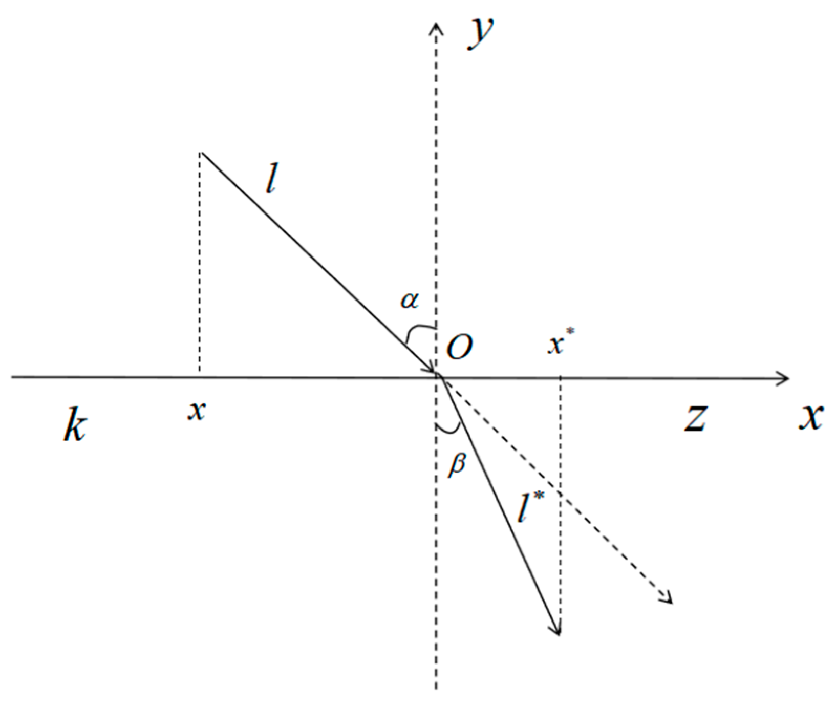
3.1. Refractive Reverse Learning Strategies

Later in the optimization search process, the DBO readily settles into local optimal solutions. The search space for dung beetle populations is expanded using a refractive reverse learning approach. To find a better alternative solution for the given problem, the search range is widened by computing the inverse solution of the existing solution. At the same time, a refraction mechanism is incorporated into reverse learning to address the issue of the DBO quickly settling into a local optimum in the latter stages of the process. Figure 1 illustrates the primary idea of this strategy.

As seen in Figure 1, the solution’s range on the $x$-axis is $[k,z]$, the $y$-axis represents the normal in the refraction reversal, the angles of incidence and refraction are represented by $\alpha$ and $\beta$, respectively, the lengths corresponding to the incident and refracted rays are represented by $l$ and $l^{\ast }$, and the origin is represented by $O$. The following is the primary formula:

$$\left\{\begin{array}{c}\sin \alpha =((k+z)/2-x)/l\\ \sin \beta =(x^{\ast }-(k+z)/2)/l^{\ast }\end{array}\right.$$

(9)

The refractive index formula is obtained by defining $n=\sin \alpha /\sin \beta$ from the refractive index formula:

$$n={\displaystyle \frac{l^{\ast }((k+z)/2-x)}{l(x^{\ast }-(k+z)/2)}}$$

(10)

Substituting the scaling factors $k=l/l^{\ast }$, $n=1$ into Equation (10) and generalizing it to the dung beetle algorithm in the high dimensional space yields the following equation:

$${x^{\ast }}_{i,j}={\displaystyle \frac{k_j+z_j}{2}}+{\displaystyle \frac{k_j+z_j}{2k}}-{\displaystyle \frac{x_{i,j}}{k}}$$

(11)

where $x_{i,j}$ is the $i\mathrm{th}$ dung beetle’s $j$-dimensional position $(i=1,2,\cdot \cdot \cdot ,N;j=1,2,\cdot \cdot \cdot ,D)$ in the population, $N$ is the number of populations, $D$ is the dimension, ${x^{\ast }}_{i,j}$ is the refractive inverse position of $x_{i,j}$, and $l_j$ and $u_j$ are the search space’s minimum and maximum values, respectively, in the $j\mathrm{th}$ dimension.

3.2. Multi-Strategy Integration Improvement

3.2.1. Adaptive Population Change

To maintain stable dung beetle populations, the program uses the breeding dung beetles to explore locally and the little dung beetles to travel the world. Therefore, the algorithm should start with better global search skills and finish with better local search capabilities. Consequently, the early edition would have more small dung beetles and fewer breeding dung beetles, whereas the late iteration would have more breeding dung beetles and fewer small dung beetles. Thus, this article suggests an adaptive change curve with a steadily increasing trend for the dung beetle population, with a value range of $P$ being [0.2, 0.6]. During the initial stages, it may produce more little dung beetles while producing fewer of them. On the other hand, as the number of iterations rises, there will be more breeding dung beetles and fewer tiny dung beetles. The following is the equation for the adaptive change curve:

$$P=0.4-0.2\times \cos (\pi \times m/M)$$

(12)

where $M$ is the algorithm’s maximum number of iterations, and $m$ is the number of iterations that are now occurring.

3.2.2. Fusion Subtractive Averaging Optimizer

When the rolling dung beetle comes across an obstruction that stops it from moving forward, it should dance to obtain a new rolling direction. To obtain a new rolling direction, this mimics the dung beetle’s dance behavior; nevertheless, this approach has the disadvantage of not having enough global search capability. Therefore, in this research, the rolling dung beetle stage incorporates the subtractive averaging optimizer when it faces an obstacle to enhance the global search stage of the DBO. The subtractive averaging optimizer is specifically described as follows.

The mathematical ideas of the average, the search agent placements, and the difference between two objective function values serve as the inspiration for the subtractive averaging optimizer. All search positions, or population members of the $t+1\mathrm{th}$ iteration, are updated using the arithmetic means of the positions of all search agents or population members of the $t\mathrm{th}$ iteration. Consequently, a unique operation “$-v$“ is introduced, which is known as subtracting search agent $i$ from search agent $z$ and is provided by the formula below:

$$x_{i,j}-x_{z,j}=sign(f(x_{i,j})-f(x_{z,j}))(x_{i,j}-\overrightarrow{v}\ast x_{z,j})$$

(13)

where $x_{i,j}$ is the $j$ dimensional location $(i,z=1,2,\cdot \cdot \cdot ,N;j=1,2,\cdot \cdot \cdot ,D)$, $N$ is the $i\mathrm{th}$ dung beetle in the population, $D$ is the dimension, and $\overrightarrow{v}$ is a vector of dimension with components that are randomly generated numbers from the set $\{1,2\}$. $\mathrm{s}\mathrm{i}\mathrm{g}\mathrm{n}$ represents the sign function, and $f(x_{i,j})$ and $f(x_{z,j})$ stand for the fitness values of the search agents $x_{i,j}$ and the $x_{z,j}$ objective functions, respectively.

Additionally, in the subtractive averaging optimizer, each search agent $x_{z,j}$ and search agent $x_{i,j}$ undergo a “$-v$” operation to obtain any search location $x_{i,j}$ in the search space. Therefore, the following is the update equation for each search agent’s new position:

$$x_i^{new}=x_i+\overrightarrow{r_i}\ast {\displaystyle \frac{1}{N}}{\displaystyle \sum _z^D(x_i-v{x}_z)},i=1,2,,\mathrm{\dots }D$$

(14)

where $\overrightarrow{r_i}$ is a vector of dimension $m$ with a normal distribution and value interval $\left[0,1\right]$, $x_i^{new}$ is the new position of the $i\mathrm{th}$ search agent, and $D$ is the total number of search agents.

3.2.3. Triangle Wandering Strategy

The introduction of a triangular wandering strategy in breeding dung beetles, which is for the walking phase of the breeding process, where the breeding dung beetles do not need to be directly close to the optimal spawning area but instead wander around the spawning area, increases the stochasticity of the breeding dung beetles, which allows the algorithm to have a better local search capability at a later stage and avoids the possibility of falling into a local optimum. Firstly, the distance between the breeding dung beetle and the spawning area is obtained $L_1$. Then, the range of walking steps of the breeding dung beetle is obtained $L_2$. The walking direction ($\beta$) of the breeding dung beetle is obtained by Equation (17). $L_1$ and $L_2$ are obtained by Equations (15) and (16), and then the distance $P$ between the position of the breeding dung beetle nowadays and the spawning area is obtained by Equation (18). Finally, the position of the breeding dung beetle after passing through the triangular wandering strategy is obtained by Equation (19).

$$L_1=po{s}_b(t)-po{s}_c(t)$$

(15)

$$\overrightarrow{L_2}=rand()\times \overrightarrow{L_1}$$

(16)

$$\beta =2\times \pi \times rand()$$

(17)

$$P={L_1}^2+{L_2}^2-2\times L_1\times L_2\times \cos (\beta )$$

(18)

$$P{\mathrm{os}}_{\mathrm{new}}=p{\mathrm{os}}_{\mathrm{b}}(t)+r\times P$$

(19)

3.3. Adaptive Gauss–Cauchy Mixed-Variance Perturbation Factor

In the late iteration of the intelligent optimization algorithm, the group of individuals will rapidly integrate and congregate close to the current optimal position, and its value is near the optimal solution. The search will stall if the group of people concentrates on the search at the current optimal position and is unable to find the genuine optimal position if the current optimal position is not the global optimal point. By employing the mutation perturbation to leap out of the present local optimum point and into other regions of the solution space to continue exploring until the global optimum is eventually found, the DBO is used in the later phases of the method. Similarly, the DBO also encounters this problem later on.

In methods for intelligent optimization, variance factors with Gaussian and Cauchy versions are commonly used. Because the Gaussian variant can generate smaller variant values with a higher probability, it has an excellent search ability in a narrow range. Compared to the Gaussian form, the Cauchy variant has a wider search range; however, its step size is excessively large, which means it will probably deviate from the ideal value and yield subpar results. Thus, this study presents the adaptive Gaussian–Cauchy hybrid perturbation variant perturbation approach, which combines the benefits of the Gaussian and Cauchy variants. Only the optimal individuals are disturbed by the variance in this paper, and the exact formula is as follows:

$$H^b(m)=X^b(m)\ast (1+{\mu }_1\ast Gauss(\sigma )+{\mu }_2\ast cauchy(\sigma ))$$

(20)

where $Gauss(\sigma )$ is the Gaussian variation operator and $cauchy(\sigma )$ is the Kersey variation factor, ${\mu }_1=m/M$, ${\mu }_1=1-m/M$.

3.4. MSFDBO Complexity Analysis

Assuming the population size of the MSFDBO algorithm is $N$, the number of iterations is $M$, and the variable dimension is $D$, we usually only focus on the highest order term of the algorithm, ignoring the constant term and low order term. The time complexity of the original DBO algorithm is $O\left(N\times D\times M\right)$. By initializing the population, the various reverse learning techniques for the MSFDBO algorithm do not make the algorithm more difficult. On the same order of magnitude as the original DBO algorithm’s time complexity, the adaptive population change, fusion subtraction average optimizer, triangle wandering strategy, and adaptive Gauss–Cauchy Mixed-Variance Perturbation Factor do not, however, increase the number of new iterations during the MSFDBO iteration process. As a result, the MSFDBO’s algorithm complexity does not rise much.

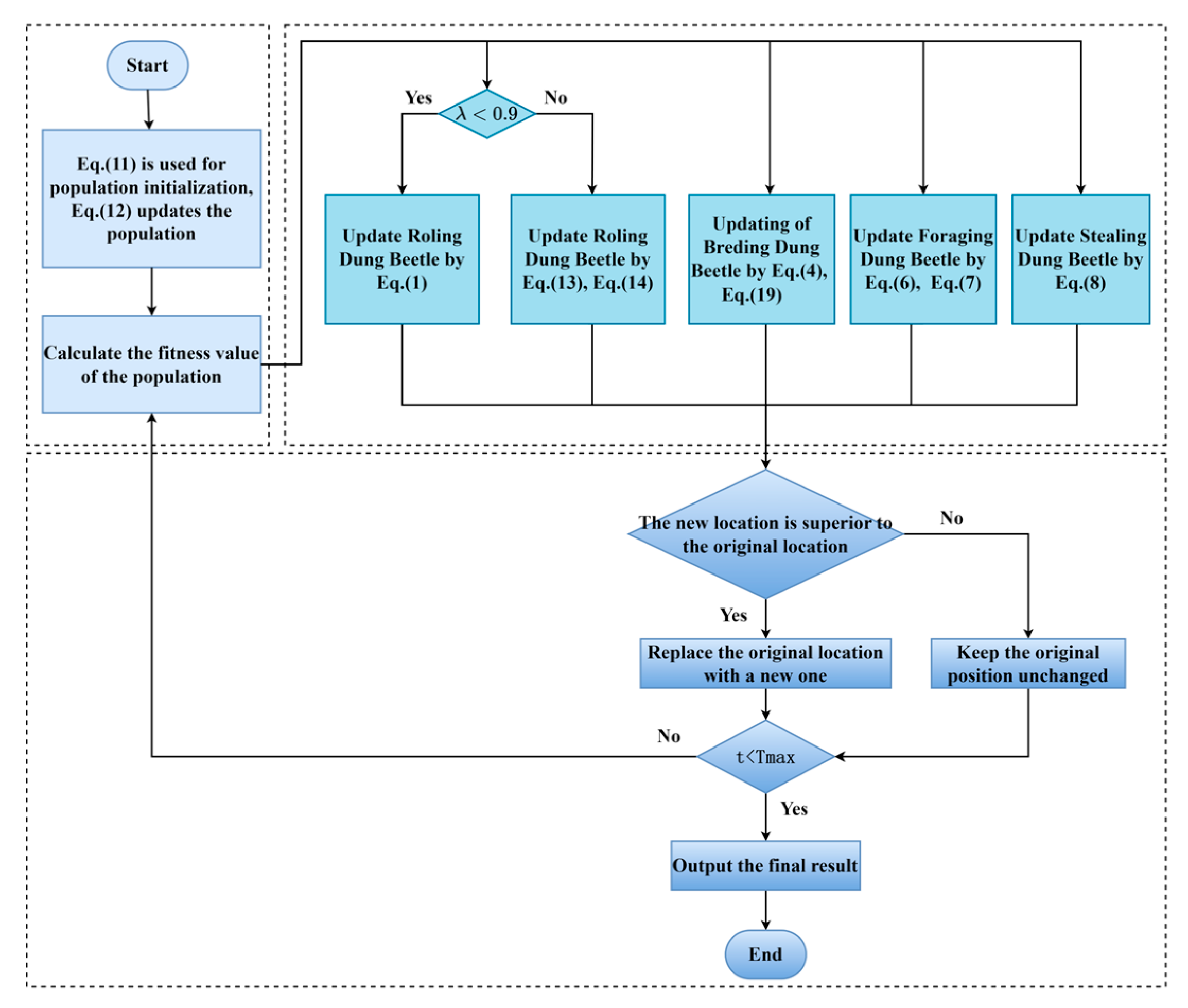
3.5. MSFDBO Algorithm Flowchart

Figure 2 shows the algorithm flowchart of the MSFDBO.

4. Experimental Results and Discussion

In this paper, the performance of the MSFDBO algorithm is tested and evaluated using seven algorithms and the results of the MSFDBO on CEC2017 test functions [26]. (It is shown in Supplementary Materials Table S1). The comparison algorithms are from the seven commonly used swarm intelligent optimization algorithms (PSO [6], SFO [27], WOA [7], SCA [28], HHO [8], SCSO [12], DBO [11]), and the algorithm parameters are shown in

Table 1. Algorithm comparison parameter setting table.

Algorithm	Parameters
PSO	ω = 1, c1 = 1.1, c2 = 1.1
SCA	a = 2
WOA	a = 2 × (1 − t/Tmax), k = 1
HHO	B = 1.5, E0 = [−1, 1]
SFO	A = 4, e = 0.001, SFP = 0.3
SCSO	rG = 2~0, =−2rG~rG
DBO	RDB = 6, EDB = 6, FDB = 7, SDB = 11
MSFDBO	R = 1 − t/Tmax

. The maximum number of iterations is set at 1000 [29], and the initialized population size of all algorithms is fixed at 30 for the experiments’ fairness. To eliminate chance in the experiments of this paper, the evaluation criterion used in this paper compares the optimal value, the mean, the standard deviation, and the ranking to the mean of the seven meta-heuristic algorithms and runs them independently 30 times on each of the test functions.

4.1. CEC2017 Benchmark Function Results and Analysis

Since the F2 function is officially removed from the list of 30 unconstrained benchmark functions in CEC2017, this article will not be conducted to present the pertinent test findings of F2. Since the outcomes of every execution of the swarm intelligence optimization algorithms are random, 30 tests were carried out for each algorithm to exclude the possibility of the experiments in this study. After 30 runs of the 50-dimension and 100-dimension CEC2017, respectively, the experimental findings and mean ranks of each method are displayed in Supplementary Materials Tables S2 and S3.

4.1.1. Analysis of CEC2017 Statistical Results

The optimal value, mean, and standard deviation of each algorithm on the benchmark test function are displayed in Tables S2 and S3 , (it is shown in the Supplementary Materials), respectively, along with the test results of this study on CEC2017 in 50 and 100 dimensions. The discussion and analysis of the experiment’s findings are provided below:

(1) The test results for the single-peak test functions F1 and F3 show that the MSFDBO intelligent optimization algorithm proposed in this paper has a better optimization-seeking ability. In the 50-dimensional test results, F1 is second only to the HHO and DBO intelligent optimization algorithms, and for F3, the optimization effect is second only to the SCSO and HHO intelligent optimization algorithms. In the 100-dimensional test results, F1 is ranked 2nd, and for F3, it is second only to SCSO and HHO intelligent optimization algorithms. The above test results show that the MSFDBO is easier to find and converge to the global optimum on the single-peak problem, which verifies that it has stronger global exploration and development capability compared to other algorithms.

(2) The experimental test results for the simple multimodal functions F4–F10 show that the MSFDBO outperforms the other seven comparative algorithms in both the 50 and 100-dimensional test results and exhibits excellent performance. In the 50-dimensional experiments, the MSFDBO outperforms the other algorithms in both F4–F6 and F8–F10, and has an order of magnitude improvement in F10, and is ranked 2nd below DBO only in F7, and also outperforms the other algorithms in the 100-dimensional experiments in both F4–F6 and F8–F10, and is only worse than DBO in F7. All these results further prove that the MSFDBO algorithm has better performance and robustness in solving complex problems.

(3) In the test results on the hybrid functions F11–F20, the MSFDBO shows significantly superior performance in dealing with hybrid problems. In the 50-dimensional experimental test results, the MSFDBO outperforms the other seven algorithms in search optimization on F11–F20, and has an order of magnitude improvement in search optimization on F12, F13, F14, F15, and F19, and is comparable to the HHO search optimization performance on F20. In the 100 dimensions, the MSFDBO outperforms the other seven algorithms in search optimization performance on F11 and F20, ranking first. On F12, the MSFDBO ranks second, with only inferior optimization performance compared to HHO. The search and optimization performance of the MSFDBO on F13–F19 has an order of magnitude improvement, which is superior to other algorithms. It can be concluded that the MSFDBO has a variety of solution search strategy options, and its strong global search performance makes it also excellent at solving hybrid problems.

(4) In solving the composite functions F21–F30, the MSFDBO is still strong and more competitive compared to other algorithms. In the 50-dimensional experimental test results, the MSFDBO outperforms other algorithms on F21, F22, F25, F26, F27, F28, F29, and F30, and the search for excellence performance is comparable to that of SCSO in F23, while in F24, the performance is poorer and ranked No. 5. whereas, in the 100-dimensional, the MSFDBO has better performance than the other algorithms on F21, F22, F27, F28, F29, and F30, the MSFDBO’s search optimization performance is better than other algorithms, while in F23, F25, and F26, it is comparable to SCSO, HHO, and DBO, respectively, and in F24, the optimization performance is worse than that of SCSO and DBO, when compared with other algorithms, the optimization performance is still advantageous. These experimental test results prove that the MSFDBO has unique advantages and adaptive performance in solving composite problems and is able to explore and search for optimality on composite problems more effectively.

Figure 3 and Figure 4 show the average degree of the algorithms on the 50 and 100 dimensions of the CEC2017 test function, respectively, and as can be seen from the figures, the MSFDBO has the first average degree.

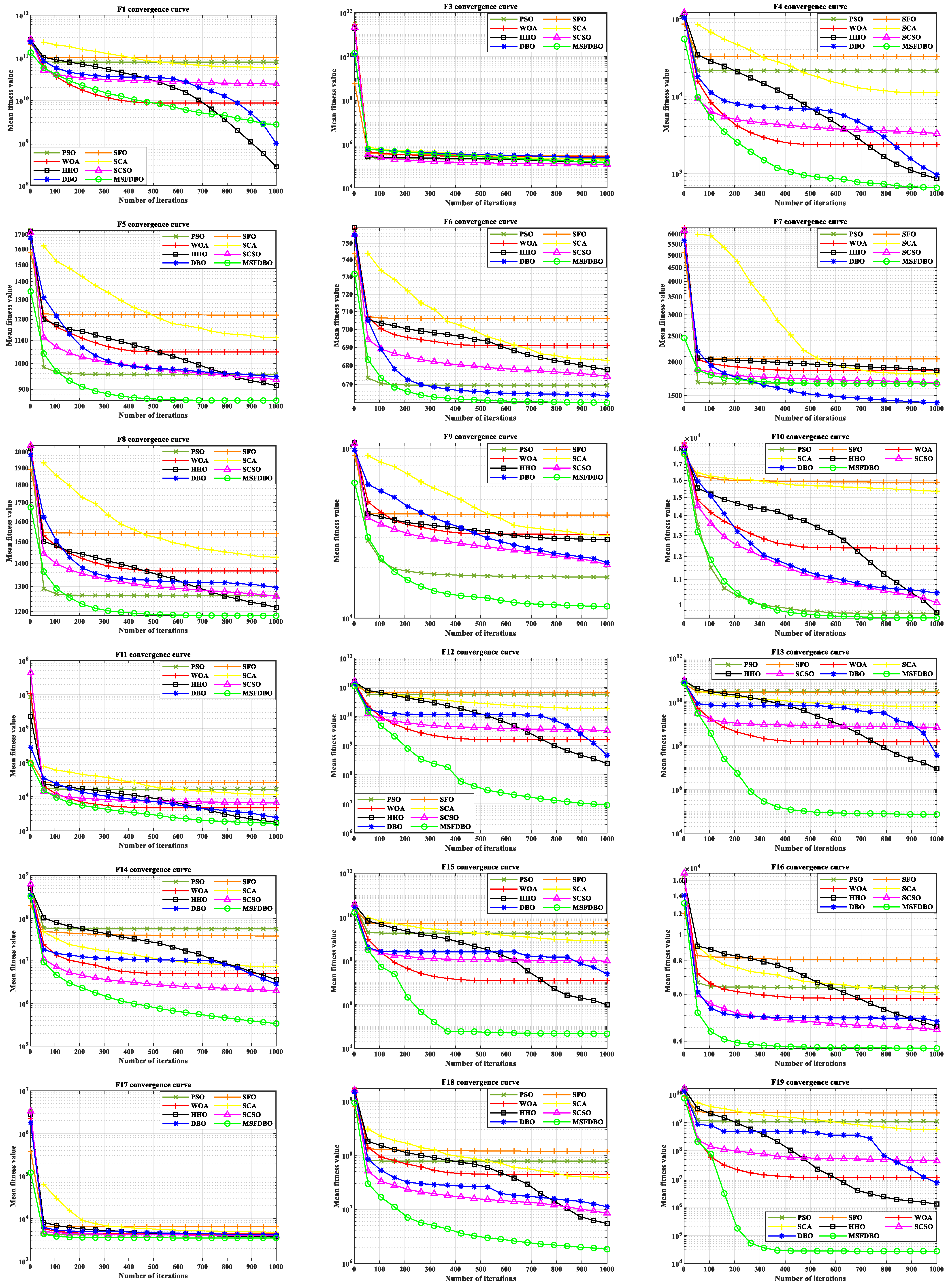
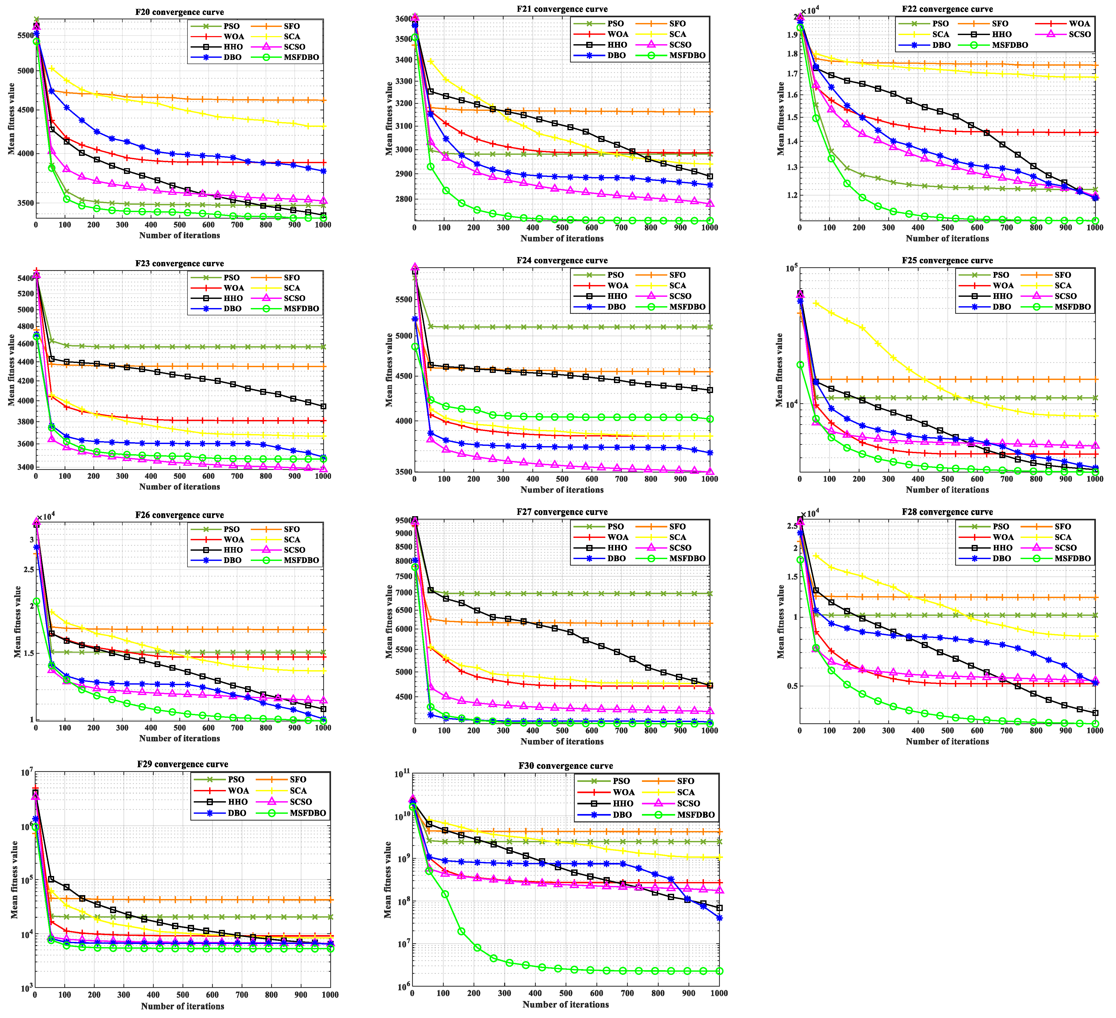
4.1.2. Comparative Analysis of CEC2017 Convergence Curves

As shown in Figure 5, the convergence curves of PSO, SFO, WOA, SCA, HHO, SCSO, and DBO are similar to those of the MSFDBO, and the MSFDBO proposed in this study outperforms the other algorithms in terms of convergence speed overall. The convergence curves are analyzed and discussed as follows:

(1) From the convergence curves of the 50-dimensional single-peaked functions F1 and F3, the convergence accuracy and convergence speed of the MSFDBO in the middle and late stages of F1 are better than the other algorithms, but the late stage of the search speeds up in HHO and DBO, which ultimately outperform the MSFDBO. However, on F3, the MSFDBO’s pre-periods have a better convergence speed than those of other algorithms.

(2) On the simple multimodal functions F4–F10, the MSFDBO suggested in this study performs significantly better than the other examined algorithms in terms of convergence accuracy and speed. DBO only overtakes it later on F7, but it still beats the other methods.

(3) On the 50-dimensional hybrid test functions F11–F20, the MSFDBO’s contraction ability progressively improves with the number of iterations, allowing it to find better solutions more quickly. Additionally, the MSFDBO’s searching ability outperforms that of the other algorithms on F12, F13, F14, F15, F16, F18, and F19, and its convergence accuracy and speed outperform those of the other algorithms throughout the iteration process. In the initial iteration, the MSFDBO outperforms the other algorithms on F11; later on, HHO and DBO improve their searching capabilities, but the MSFDBO remains at the top. The MSFDBO ranks first in F17 after having the best early searching ability and continuing to maintain a high convergence speed in subsequent iterations. In the early and middle phases, HHO’s convergence speed ranks fourth in F20; however, in the later stages, it significantly improves and quickly approaches the MSFDBO, although it still falls short of the MSFDBO and ranks second.

(4) It can be inferred from the convergence curve graphs of composite functions F21–F30 that the MSFDBO outperforms the other methods under comparison in terms of convergence accuracy and speed in F21–F22 and F30. The MSFDBO performs well in the early stages of iteration in F23, F24, F25, F26, and F29, although other algorithms eventually catch up to or even outperform it. Early on, the MSFDBO’s convergence speed on F27 is marginally slower than DBO’s, but as the number of iterations increases in the middle and late stages, the MSFDBO’s search speed dramatically increases and eventually overtakes DBO. Additionally, the MSFDBO outperforms the other algorithms in F28 in terms of convergence speed and accuracy. However, as iterations go, the other algorithms start to converge more slowly but still outperform the MSFDBO.

In conclusion, the MSFDBO demonstrates its flexibility and resilience to a variety of problem domains and levels of complexity by successfully completing the exploration of optimal values in the test function. It is also easier to converge to the global optimal solution when the MSFDBO is compared to other algorithms because it performs better in both local exploitation and global exploration.

4.2. Wilcoxon Rank Sum Test

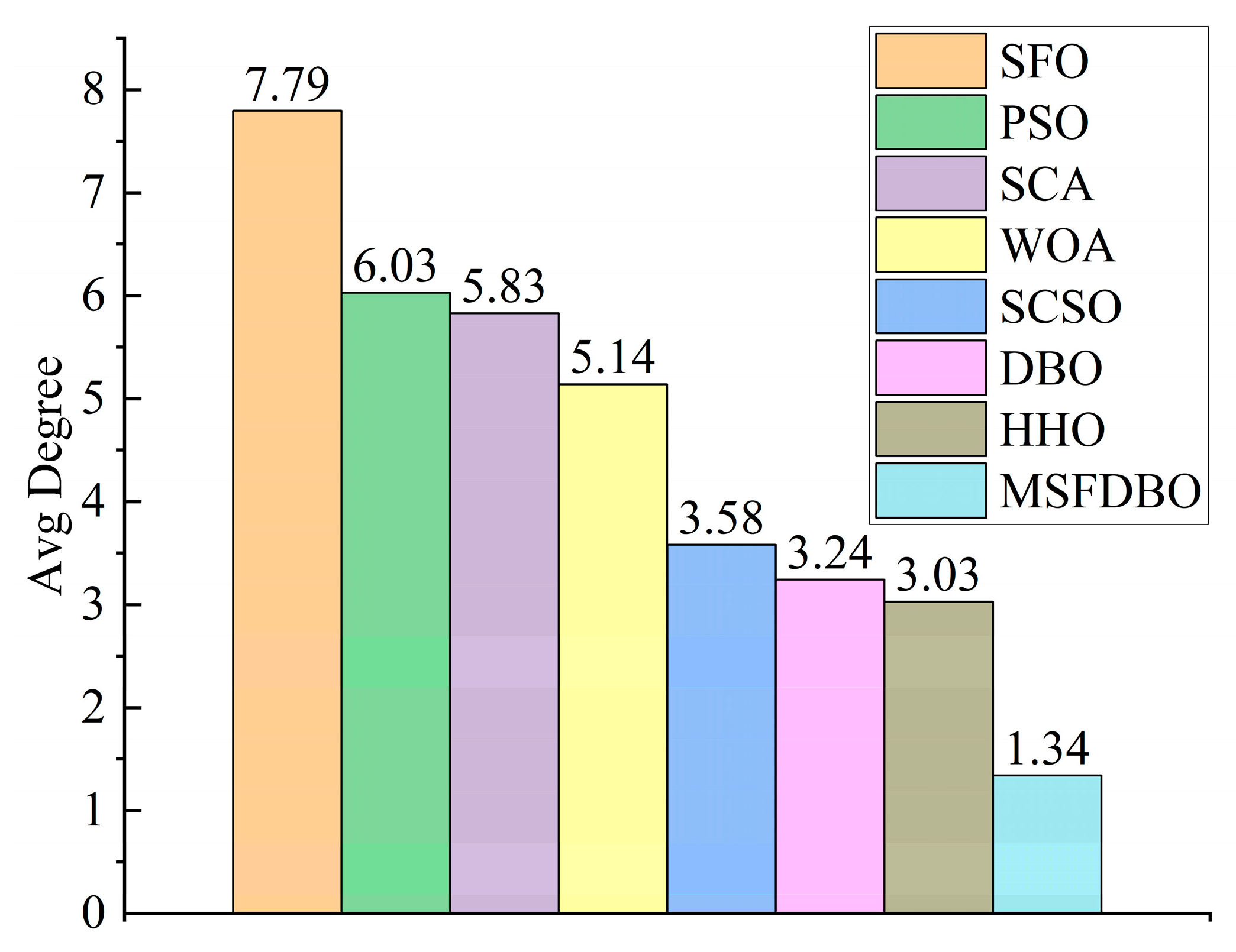
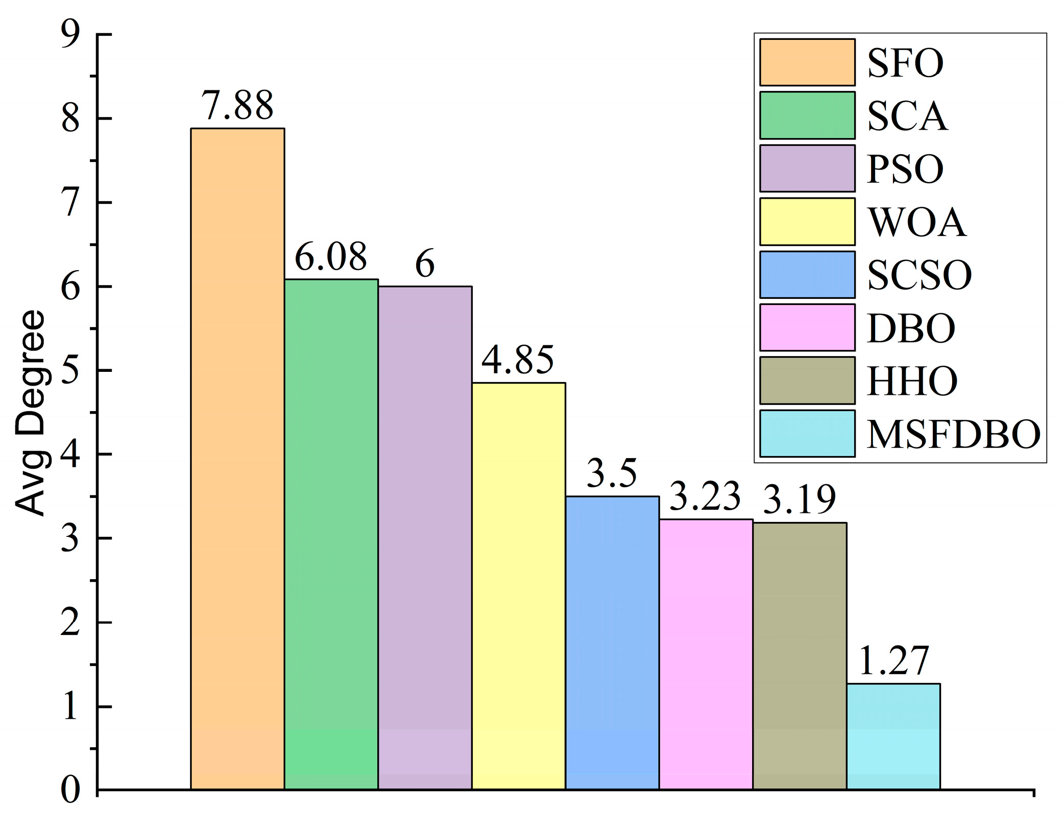
Although thirty different runs are used to compare the performances of the different algorithms, additional statistical testing is still required to fully understand their capabilities. The Wilcoxon rank sum test is used to assess whether the results of each MSFDBO run are significantly different from those of the other algorithms at the p = 5% significance level. According to the null hypothesis, there should not be much difference between each pair of algorithms. p > 5% signifies the acceptance of the original hypothesis, implying that the two compared algorithms perform similarly; N/A indicates that the intelligent optimization algorithms perform similarly in terms of optimizing the search process and are not comparable; and p < 5% indicates the rejection of the original hypothesis, implying that a notable distinction is present between the two tested algorithms. The exact test results obtained for the MSFDBO by utilizing each competing method independently are displayed in Tables S4 and S5. (It is shown in the Supplementary Materials).

4.3. Friedman Test

Each optimization algorithm’s ranking is determined by the Friedman test, and each swarm intelligence optimization method is then put through the Friedman test based on its ranking on the test function in Tables S2 and S3.

Table 2. Friedman test.

Test Function	PSO	SFO	WOA	SCA	HHO	SCSO	DBO	MSFDBO
CEC2017 50D	6.0345	7.7931	5.1379	5.8276	3.0345	3.5862	3.2414	1.3448
CEC2017 100D	6.0690	7.7586	4.8966	6.0345	3.0345	3.5172	3.3448	1.3448

displays the test results. The success of the modification is demonstrated by the data in Table 2, which shows that the MSFDBO’s average ranking is lower than that of other algorithms.

5. Engineering Application Design Issues

Algorithm research aims to solve real-world engineering challenges; good performance in test functions does not entirely translate to algorithm performance in real-world problems. Therefore, the welded beam design problem [30] and the reducer design problem [31] will be used in this section’s investigation of the MSFDBO to confirm its effectiveness.

5.1. Welded Beam Design Issues

The objective of the practical engineering problem of welded beam design is to guarantee safety performance while lowering the welded beam’s production cost. The optimization of the welded sorghum problem requires that the limitations of shear stresses ($\tau$), bending stresses within the sorghum ($\sigma$), buckling loads ($P\mathrm{c}$), sorghum disturbance ($\delta$), and lateral limits be met. Additionally, four important variables—width ($\mathrm{t}$), weld thickness ($\mathrm{h}$), length ($\mathrm{l}$), and thickness ($\mathrm{b}$)—have an impact on the cost of making welded sorghum. The following is also stated in mathematical notation, (it is shown in the Supplementary Materials,) as illustrated in Figure 6.

By comparing the MSFDBO proposed in this paper with PSO, SCA, WOA, HHO, SFO, SCSO, and DBO, the total design cost of the MSFDBO is minimized, as shown in

Table 3. Comparison of test results of algorithms for solving the welded sorghum problem.

Arithmetic	$\mathit{h}$	$\mathit{l}$	$\mathit{t}$	$\mathbf{b}$	Cost Optimization
PSO	0.1525	6.0671	9.7399	0.2025	2.0597
SFO	0.1710	4.8328	8.2402	0.2545	2.0189
WOA	0.1580	6.4434	9.5400	0.2034	2.0850
SCA	0.2010	3.5951	9.5716	0.2107	1.8645
HHO	0.1682	4.8085	8.9901	0.2169	1.9105
SCSO	0.2009	3.3397	9.0395	0.2057	1.7003
DBO	0.2035	3.0899	9.5183	0.2036	1.7331
MSFDBO	0.2057	3.2444	9.0337	0.2059	1.6948

.

5.2. Reducer Design Issues

Optimizing the weight and axial deformation of the gears in order to minimize the reducer’s overall weight is the aim of the reducer design challenge. The width of the shaft face ($b=x_1$), the number of tooth molds ($m=x_2$), the number of teeth on the pinion ($p=x_3$), the length of the first shaft between the bearings ($l_1=x_4$), the length of the second shaft between the bearings ($l_2=x_5$), the diameter of the first shaft ($d_1=x_6$) and the diameter of the second shaft ($d_2=x_7$) are the seven constraint variables that affect the reducer, as shown in Figure 7. The pertinent design variables and the reducer’s weight are also determined by resolving the reducer’s eleven constraints. The following is also stated in the mathematical notation. (It is shown in the Supplementary Materials).

By comparing the MSFDBO proposed in this paper with SCA, WOA, HHO, SFO, SCSO, and DBO, it can be seen from

Table 4. Comparison of test results of each algorithm for solving the reducer problem.

Algorithms	${\mathit{x}}_1$	${\mathit{x}}_2$	${\mathit{x}}_3$	${\mathit{x}}_4$	${\mathit{x}}_5$	${\mathit{x}}_6$	${\mathit{x}}_7$	Optimum Weight
PSO	3.6000	0.7000	17.0000	8.3000	8.3000	3.4122	5.3642	3121.9650
SFO	3.5114	0.7000	18.2404	7.5813	7.7169	3.5598	5.2878	3281.4934
WOA	3.5355	0.7000	17.0000	7.8000	7.8464	3.6251	5.3290	3126.6302
SCA	3.6000	0.7000	17.0000	7.3000	8.1063	3.4789	5.3751	3134.3656
HHO	3.5000	0.7000	17.0000	7.6652	7.9002	3.5581	5.3308	3086.9231
SCSO	3.5015	0.7000	17.0001	7.6361	7.8095	3.3526	5.2888	3002.0753
DBO	3.6000	0.7000	17.0000	7.3000	8.3000	3.3502	5.2869	3046.7137
MSFDBO	3.5000	0.7000	17.0000	7.3000	7.7153	3.3502	5.2867	2994.4711

that the MSFDBO algorithm obtains the minimum weight of the reducer when dealing with the reducer design problem, which effectively saves the engineering design cost.

6. Conclusions

The MSFDBO proposed makes use of an adaptive Gaussian–Cauchy mixed-variance perturbation factor strategy, triangle wandering technique, and fusion subtractive averaging optimizer. A Wilcoxon rank sum test was performed on the complicated function set CEC2017, with a variety of features for assessing the MSFDBO’s improved performance. Two challenging engineering application design difficulties were finally resolved using the MSFDBO approach. When compared to the top-performing algorithms, the experimental findings demonstrate that the MSFDBO has significant engineering application ability. In the future, we will also use the MSFDBO to select highly correlated features from high-dimensional data, as well as to optimize neural network parameters and plan paths. This will show that the MSFDBO is a useful tool for high-dimensional and large-scale optimization problems.

References

1. Liu, A.; Jiang, J. Solving path planning problem based on logistic beetle algorithm search–pigeon-inspired optimisation algorithm. Electron. Lett. 2020, 56, 1105–1108. [Google Scholar] [CrossRef]
2. Huang, Q.; Ding, H.; Razmjooy, N. Oral cancer detection using convolutional neural network optimized by combined seagull optimization algorithm. Biomed. Signal Process. Control. 2024, 87, 105546. [Google Scholar] [CrossRef]
3. Luo, X.; Du, B.; Gui, P.; Zhang, D.; Hu, W. A Hunger Games Search algorithm with opposition-based learning for solving multimodal medical image registration. Neurocomputing 2023, 540, 126204. [Google Scholar] [CrossRef]
4. Shen, Y.; Zhang, C.; Gharehchopogh, F.S.; Mirjalili, S. An improved whale optimization algorithm based on multi-population evolution for global optimization and engineering design problems. Expert Syst. Appl. 2023, 215, 119269. [Google Scholar] [CrossRef]
5. Zhang, N.; Cai, Y.X.; Wang, Y.Y.; Tian, Y.T.; Wang, X.L.; Badami, B. Skin cancer diagnosis based on optimized convolutional neural network. Artif. Intell. Med. 2020, 102, 101756. [Google Scholar] [CrossRef] [PubMed]
6. Kennedy, J.; Eberhart, R. Particle swarm optimization. In Proceedings of the ICNN'95-International Conference on Neural Networks, Perth, WA, Australia, 27 November–1 December 1995; IEEE: Piscataway, NJ, USA, 1995; Volume 4, pp. 1942–1948. [Google Scholar]
7. Mirjalili, S.; Mirjalili, S.M.; Lewis, A. Grey wolf optimizer. Adv. Eng. Softw. 2014, 69, 46–61. [Google Scholar] [CrossRef]
8. Mirjalili, S.; Lewis, A. The whale optimization algorithm. Adv. Eng. Softw. 2016, 95, 51–67. [Google Scholar] [CrossRef]
9. Heidari, A.A.; Mirjalili, S.; Faris, H.; Aljarah, I.; Mafarja, M.; Chen, H. Harris hawks optimization: Algorithm and applications. Future Gener. Comput. Syst. 2019, 97, 849–872. [Google Scholar] [CrossRef]
10. Jain, M.; Singh, V.; Rani, A. A novel nature-inspired algorithm for optimization: Squirrel search algorithm. Swarm Evol. Comput. 2019, 44, 148–175. [Google Scholar] [CrossRef]
11. Xue, J.; Shen, B. A novel swarm intelligence optimization approach: Sparrow search algorithm. Syst. Sci. Control Eng. 2020, 8, 22–34. [Google Scholar] [CrossRef]
12. Xue, J.; Shen, B. Dung beetle optimizer: A new meta-heuristic algorithm for global optimization. Ournal Supercomput. 2023, 79, 7305–7336. [Google Scholar] [CrossRef]
13. Seyyedabbasi, A.; Kiani, F. Sand Cat swarm optimization: A nature-inspired algorithm to solve global optimization problems. Eng. Comput. 2023, 39, 2627–2651. [Google Scholar] [CrossRef]
14. Hashim, F.A.; Hussien, A.G. Snake Optimizer: A novel meta-heuristic optimization algorithm. Knowl.-Based Syst. 2022, 242, 108320. [Google Scholar] [CrossRef]
15. Chopra, N.; Ansari, M.M. Golden jackal optimization: A novel nature-inspired optimizer for engineering applications. Expert Syst. Appl. 2022, 198, 116924. [Google Scholar] [CrossRef]
16. Wolpert, D.H.; Macready, W.G. No free lunch theorems for optimization. IEEE Trans. Evol. Comput. 1997, 1, 67–82. [Google Scholar] [CrossRef]
17. Zhu, F.; Li, G.; Tang, H.; Li, Y.; Lv, X.; Wang, X. Dung beetle optimization algorithm based on quantum computing and multi-strategy fusion for solving engineering problems. Expert Syst. Appl. 2024, 236, 121219. [Google Scholar] [CrossRef]
18. Duan, Y.; Yu, X. A collaboration-based hybrid GWO-SCA optimizer for engineering optimization problems. Expert Syst. Appl. 2023, 213, 119017. [Google Scholar] [CrossRef]
19. Sahoo, S.K.; Saha, A.K.; Nama, S.; Masdari, M. An improved moth flame optimization algorithm based on modified dynamic opposite learning strategy. Artif. Intell. Rev. 2023, 56, 2811–2869. [Google Scholar] [CrossRef]
20. Yan, S.; Yang, P.; Zhu, D.; Zheng, W.; Wu, F. Improved sparrow search algorithm based on iterative local search. Comput. Intell. Neurosci. 2021, 2021, 6860503. [Google Scholar] [CrossRef] [PubMed]
21. Li, Y.; Sun, K.; Yao, Q.; Wang, L. A dual-optimization wind speed forecasting model based on deep learning and improved dung beetle optimization algorithm. Energy 2024, 286, 129604. [Google Scholar] [CrossRef]
22. Wang, S.; Cao, L.; Chen, Y.; Chen, C.; Yue, Y.; Zhu, W. Gorilla optimization algorithm combining sine cosine and cauchy variations and its engineering applications. Sci. Rep. 2024, 14, 7578. [Google Scholar] [CrossRef] [PubMed]
23. Ewees, A.A.; Mostafa, R.R.; Ghoniem, R.M.; Gaheen, M.A. Improved seagull optimization algorithm using Lévy flight and mutation operator for feature selection. Neural Comput. Appl. 2022, 34, 7437–7472. [Google Scholar] [CrossRef]
24. Zhang, Y.; Lin, J.; Hu, Z.; Khan, N.A.; Sulaiman, M. Analysis of third-order nonlinear multi-singular Emden–Fowler equation by using the LeNN-WOA-NM algorithm. IEEE Access 2021, 9, 72111–72138. [Google Scholar] [CrossRef]
25. Zhang, R.; Zhu, Y. Predicting the mechanical properties of heat-treated woods using optimization-algorithm-based BPNN. Forests 2023, 14, 935. [Google Scholar] [CrossRef]
26. Guohua, W.; Rammohan, M.; Suganthan, P. Problem Definitions and Evaluation Criteria for the CEC 2017 Competition and Special Session on Constrained Single Objective Real-Parameter Optimization; Nanyang Technological University: Singapore, 2016. [Google Scholar]
27. Shadravan, S.; Naji, H.R.; Bardsiri, V.K. The Sailfish Optimizer: A novel nature-inspired metaheuristic algorithm for solving constrained engineering optimization problems. Eng. Appl. Artif. Intell. 2019, 80, 20–34. [Google Scholar] [CrossRef]
28. Mirjalili, S. SCA: A sine cosine algorithm for solving optimization problems. Knowl.-Based Syst. 2016, 96, 120–133. [Google Scholar] [CrossRef]
29. Jia, H.; Peng, X.; Lang, C. Remora optimization algorithm. Expert Syst. Appl. 2021, 185, 115665. [Google Scholar] [CrossRef]
30. Fan, Q.; Chen, Z.; Zhang, W.; Fang, X. ESSAWOA: Enhanced whale optimization algorithm integrated with salp swarm algorithm for global optimization. Eng. Comput. 2022, 38 (Suppl. S1), 797–814. [Google Scholar] [CrossRef]
31. Zhao, Y.; Huang, C.; Zhang, M.; Lv, C. COLMA: A chaos-based mayfly algorithm with opposition-based learning and Levy flight for numerical optimization and engineering design. Ournal Supercomput. 2023, 79, 19699–19745. [Google Scholar] [CrossRef]
Figure 1. Refractive inverse learning schematics.
Electronics 14 00197 g001
Figure 2. MSFDBO algorithm flowchart.
Electronics 14 00197 g002
Figure 3. CEC2017 50 dimension average degree levels.
Electronics 14 00197 g003
Figure 4. CEC2017 100 dimension average degree levels.
Electronics 14 00197 g004
Figure 5. Average convergence curves of CEC2017 50-dimensional benchmarking functions.
Electronics 14 00197 g005aElectronics 14 00197 g005b
Figure 6. Schematic of the welded beam (Above: Engineering drawing, Below: 3D).
Electronics 14 00197 g006
Figure 7. Schematic of the reducer design (Right: Engineering drawing, Left: 3D).
Electronics 14 00197 g007