Bayesian Adaptive Detection for Distributed MIMO Radar with Insufficient Training Data

Abstract

The distributed multiple-input multiple-output (MIMO) radar observes targets from different angles, which can overcome the adverse effects of target glint and avoid the situation where the target’s tangential flight cannot be effectively detected by the radar, thus providing great advantages in target detection. However, distributed MIMO often encounters a scarcity of training samples for target detection. To overcome this difficulty, this paper proposes a Bayesian approach. By modeling the target signal as a subspace signal, where each transmit–receive pair possesses a distinct and unknown covariance matrix governed by an inverse Wishart distribution, three efficient detectors are devised based on the generalized likelihood ratio test (GLRT), Rao, and Wald criteria. Comparative analysis with existing detectors reveals that the proposed Bayesian detectors exhibit superior performance, particularly in scenarios with limited training data. Experimental results demonstrate that the Bayesian GLRT achieves the highest probability of detection (PD), outperforming conventional detectors by requiring a reduction in signal-to-noise ratio (SNR). Furthermore, an increase in the degrees of freedom of the inverse Wishart distribution and the number of receiving antennas enhances detection performance, albeit at the cost of increased hardware requirements.

1. Introduction

With the advancement of technology, radar systems have continued to diversify, and their functions have expanded significantly. However, target detection remains one of the most fundamental and crucial functions of radar [1,2]. Multiple-input multiple-output (MIMO) radar, as a typical example of a new-generation radar, employs multiple antennas to transmit distinct waveforms, thereby offering transmit degrees of freedom, heightened flexibility, and immense potential for enhanced detection performance [3,4]. MIMO radar encompasses two fundamental categories: colocated MIMO radar [5,6] and distributed MIMO radar [7,8].

The antennas of the colocated MIMO radar are closely packed together, and by transmitting different waveforms, higher spatial resolution and more flexible beam control can be achieved [9]. The distributed MIMO radar observes targets from different angles, which can greatly reduce the performance loss caused by target fluctuation on radar detection [10]. This paper mainly focuses on the study of distributed MIMO radar. For the convenience of description, the MIMO radar in the following text refers to the distributed MIMO radar.

The advancement of target detection strategies in MIMO radar has been a subject of recent research, with various studies contributing to the field [11,12,13,14]. Research indicates that MIMO radar can leverage target spatial diversity to enhance detection, as demonstrated in [15]. Space–time coding (STC) is explored as a means to achieve diversity and improve detection in [16]. A tradeoff between diversity and integration is highlighted in [17], suggesting the absence of a universally optimal waveform for detection. The generalized likelihood ratio test (GLRT) for MIMO radar is derived in [18], assuming a consistent number of training data across different transmit–receive pairs, and is shown to outperform phased array systems. This derivation is generalized in [19], which removes the constraint on the number of training data for different transmit–receive pairs and provides a formula for the probability of false alarm (PFA). Registration errors in MIMO radar detection, which occur when aligning data from distributed radars into a common coordinate system, are addressed in [20], where effective detectors are proposed that surpass conventional methods under imperfect registration. The study in [20] introduces a two-stage detection approach with a local threshold to regulate the communication rate and a global threshold to set the overall PFA. In [21], a GLRT is introduced for moving target detection using colocated MIMO radar on multiple distributed moving platforms. Simulations showcase the superiority of this radar system in detecting moving targets compared to existing distributed and colocated MIMO radars. In [22], the detection problem in distributed MIMO radar is addressed when the environment is partially homogeneous in each transmitter–receiver path and non-homogeneous for different paths. By modeling disturbance signals as auto-regressive (AR) processes, two parametric detectors are developed using the Wald test. In [23], the authors examine the challenge of joint target detection and clutter mitigation in distributed MIMO radar that employs nonorthogonal waveforms. They introduce three types of detection solutions: noncoherent detectors, coherent detectors, and hybrid detectors, which offer a balance between the first two approaches.

In the majority of the aforementioned references concerning MIMO radar detection, the assumption is often made that either the covariance matrices across different range bins are identical or that there are sufficient amounts of training data available to estimate the covariance matrix. In reality, it is common to encounter scenarios where the clutter in different resolution cells or transmit–receive pairs displays distinct characteristics [24]. These location-dependent clutter traits result in heterogeneity, with the covariance matrix varying across different resolution cells. Consequently, there tends to be a limited amount of independent and identically distributed (IID) training data available to form a reliable estimate of the unknown covariance matrix. To address the challenge posed by limited training data, two types of detectors are introduced in [25]. The first is a sparsity-based detector that leverages the sparse representation of clutter in the Doppler domain. The second is an adaptive parametric detector that utilizes a parametric autoregressive clutter model. Both detectors are designed under the assumption that clutter is confined to a specific subspace. However, the complexity of clutter in real-world environments may not align with these constraints. To tackle this issue, the Bayesian theory is applied in [26] by assuming that the covariance matrix follows an inverse Wishart distribution governed by an appropriate scale matrix, which can be derived from antenna configuration or historical data.

Note that several limitations are present in the approach outlined in [26]. Firstly, it assumes that the covariance matrices between different transmit–receive pairs maintain the same structure, differing only in power levels. In actual scenarios, because MIMO radar observes targets from various angles, the covariance matrices for different transmit–receive pairs not only vary in power levels but also in structure. Secondly, the detectors proposed are specifically designed for rank-one signals. However, due to actions such as target maneuvering and turning, it is often challenging to accurately model the target signal with a rank-one model, necessitating a more robust subspace model instead. Lastly, only the GLRT criterion is used in [26]. Given the complexity of the problem, with a multitude of unknowns, there is no uniformly most powerful (UMP) test. Therefore, it may be beneficial to explore alternative criteria beyond the GLRT for detector design.

Based on the above considerations, this paper uses Bayesian theory to solve the problem of target detection in MIMO radar when training samples are insufficient. Specifically, the target signal is modeled as a subspace signal, and each transmit–receive pair has a different unknown covariance matrix. The covariance matrix is ruled by a different inverse Wishart distribution. Based on the GLRT, Rao, and Wald criteria, three effective detectors are designed and compared with existing detectors. The results show that the performance of the designed detectors is superior to existing detectors.

2. Problem Formulation

Suppose that the MIMO radar includes M transmit antennas and N receive antennas. Each transmit antenna transmits K coherent pulses within a coherent processing interval (CPI), and the waveforms transmitted by different antennas are orthogonal. After matched filtering, the pulse-echo data transmitted by the mth transmitting antenna and received by the nth receiving antenna can be represented as a K × 1 dimensional column vector $x_{mn}$. Under hypothesis H₀, $x_{mn}$ only contains noise $n_{mn}$, while under hypothesis H₁, $x_{mn}$ also contains signal $s_{mn}^{\prime }$, expressed as $s_{mn}^{\prime }={\beta }_{mn}{s}_{mn}$, with ${\beta }_{mn}$ and $s_{mn}$ being signal amplitude and signal steering vector, respectively. $s_{mn}$ has the form $s_{mn}={[1,{\mathrm{e}}^{-j2\pi f_{mn}{T}_{\mathrm{r}}},\cdots ,{\mathrm{e}}^{-j2\pi (K-1)f_{mn}{T}_{\mathrm{r}}}]}^T$, where T_r is pulse repetition frequency (PRF), $f_{mn}$ is the target Doppler frequency, and ${(\cdot )}^T$ denotes transpose.

In the real environment, due to the maneuvering flight of the target and other reasons, there usually exists uncertainty in the target’s Doppler frequency. To overcome this problem, a feasible idea is to use a subspace model to characterize the Doppler steering vector of the target. In other words, it is assumed that the target Doppler steering vector is located in a given subspace. It follows that we can model $s_{mn}$ as $s_{mn}=H_{mn}{\mathsf{\alpha }}_{mn}$, where $H_{mn}$ is a $K\times p$ full-column-rank signal matrix and ${\mathsf{\alpha }}_{mn}$ is the $p\times 1$ coordinate vector. Suppose that $n_{mn}$ is zero-mean, Gaussian distributed, with covariance matrix $R_{mn}$, which is usually unknown. To estimate $R_{mn}$, a certain number of training data are needed. Let $y_{l_{mn}}$ be the $l_{mn}$ th training data, which only contain noise $w_{l_{mn}}$, $l_{mn}=1,2,\cdots ,L_{mn}$, with $L_{mn}$ being the number of the training data. $w_{l_{mn}}$ shares the same covariance matrix $R_{mn}$. To sum up, the detection problem can be expressed as

$$\left\{\begin{array}{l}{\mathrm{H}}_0:x_{mn}=n_{mn}, y_{l_{mn}}=w_{l_{mn}},\\ m=1,\cdots ,M,n=1,\cdots ,N,l_{mn}=1,\cdots ,L_{mn}\\ {\mathrm{H}}_1:x_{mn}=H_{mn}{\mathsf{\alpha }}_{mn}+n_{mn}, y_{l_{mn}}=w_{l_{mn}},\\ m=1,\cdots ,M,n=1,\cdots ,N,l_{mn}=1,\cdots ,L_{mn}\end{array}\right.$$

(1)

It is noteworthy to emphasize that for an accurate estimation of $R_{mn}$, the quantity of training data, $L_{mn}$, must be sufficiently large. At least, $L_{mn}$ is greater than or equal to K to ensure that the sample covariance matrix (SCM) is nonsingular. However, in practice, the above requirement is often difficult to meet due to the heterogeneous characteristics of the environment.

To solve the detection problem when the training samples are insufficient, i.e., $\min {\left\{L_{mn}\right\}}_{m,n=1}^{M,N}<K$, this paper designs adaptive detectors for MIMO radar based on Bayesian theory. Specifically, $R_{mn}$ follows an inverse Wishart distribution with ${\mu }_{mn}$ degrees of freedom (DOFs), and a scalar matrix ${\mu }_{mn}{\mathsf{\Sigma }}_{mn}$, denoted as

$$R_{mn}~\mathcal{C}{\mathcal{W}}_K^{-1}\left({\mu }_{mn},{\mu }_{mn}{\mathsf{\Sigma }}_{mn}\right)$$

(2)

It is known that $\mathrm{E}[R_{mn}]=[{\mu }_{mn}/({\mu }_{mn}-K)]{\mathsf{\Sigma }}_{mn}$ and $\mathrm{E}[{‖R_{mn}-{\mathsf{\Sigma }}_{mn}‖}^2]\approx {\mathrm{tr}}^2({\mathsf{\Sigma }}_{mn})/{\mu }_{mn}$ [27], where the symbol E[·] denotes a statistical expectation. From the above two equations, it can be seen that the greater the DOF ${\mu }_{mn}$, the higher the credibility of the prior information for $R_{mn}$.

3. Detector Design

We derive the Bayesian GLRT, Rao, and Wald tests in sequence in this Section.

3.1. GLRT

For the detector problem in (1), the joint probability density function (PDF) for fixed $R_{mn}$ is

$${\displaystyle \prod _{m=1}^M{\displaystyle \prod _{n=1}^N{\displaystyle \prod _{l_{mn}=1}^{L_{mn}}{f}_1(x_{mn},y_{l_{mn}}|R_{mn})}}}={\displaystyle \prod _{m=1}^M{\displaystyle \prod _{n=1}^N\frac{\exp \left[-x_{mn,1}^H{R}_{mn}^{-1}{x}_{mn,1}-\mathrm{tr}(S_{mn}{R}_{mn}^{-1})\right]}{{\pi }^{K(L_{mn}+1)}|R_{mn}{|}^{L_{mn}+1}}}}$$

(3)

where $x_{mn,1}=x_{mn}-H_{mn}{\mathsf{\alpha }}_{mn}$, $S_{mn}={\displaystyle {\sum }_{l_{mn}=1}^{L_{mn}}{y}_{l_{mn}}{y}_{l_{mn}}^H}$, $\mathrm{tr}(\cdot )$ is the matrix trace, and $|\cdot |$ is the matrix determinant.

The Bayesian GLRT can be written as

$$t_{\mathrm{GLRT}}={\displaystyle \frac{\underset{{\mathsf{\alpha }}_{mn}, R_{mn}}{\max }{\displaystyle \prod _{m=1}^M{\displaystyle \prod _{n=1}^N{\displaystyle \prod _{l_{mn}=1}^{L_{mn}}{f}_1(x_{mn},y_{l_{mn}}|R_{mn})f(R_{mn})\mathrm{d}{R}_{mn}}}}}{\underset{{\mathsf{\alpha }}_{mn}, R_{mn}}{\max }{\displaystyle \prod _{m=1}^M{\displaystyle \prod _{n=1}^N{\displaystyle \prod _{l_{mn}=1}^{L_{mn}}{f}_0(x_{mn},y_{l_{mn}}|R_{mn})f(R_{mn})\mathrm{d}{R}_{mn}}}}}}$$

(4)

where the PDF $f(R_{mn})$ is found to be [28]

$$f(R_{mn})={\displaystyle \frac{|{\mathsf{\Sigma }}_{mn}{|}^{{\mu }_{mn}}}{c|R_{mn}{|}^{{\mu }_{mn}+N}}}\mathrm{etr}(-{\mu }_{mn}{\mathsf{\Sigma }}_{mn}{R}_{mn}^{-1})$$

(5)

with $c={\pi }^{K(K-1)/2}{\displaystyle \prod _{i=1}^K\Gamma ({\mu }_{mn}-K+i)}$. It follows from Equations (3) and (5) that

$${\displaystyle \prod _{l_{mn}=1}^{L_{mn}}{f}_1(x_{mn},y_{l_{mn}}|R_{mn})}f(R_{mn})=c|{\mathsf{\Sigma }}_{mn}{|}^{{\mu }_{mn}}{\displaystyle \frac{\mathrm{etr}\left[-R_{mn}^{-1}(x_{mn,1}{x}_{mn,1}^H+S_{mn}+{\mu }_{mn}{\mathsf{\Sigma }}_{mn})\right]}{|R_{mn}{|}^{{\mu }_{mn}+K+L_{mn}+1}}}$$

(6)

Performing integration of Equation (6) with respect to (w.r.t.) $R_{mn}$ results in

$${\displaystyle \int {\displaystyle \prod _{l_{mn}=1}^{L_{mn}}{f}_1(x_{mn},y_{l_{mn}}|R_{mn})}f(R_{mn})\mathrm{d}{R}_{mn}}=c{\lambda }^{-K}|\mathsf{\Sigma }{|}^{{\mu }_{mn}}{\left|x_{mn,1}{x}_{mn,1}^H+S_{mn}+{\mu }_{mn}{\mathsf{\Sigma }}_{mn}\right|}^{-({\mu }_{mn}+L_{mn}+1)}$$

(7)

Taking Equation (7) into Equation (4) leads to

$$t_{\mathrm{B}\text{-}\mathrm{GLRT}}={\displaystyle \frac{{\displaystyle \prod _{m=1}^M{\displaystyle \prod _{n=1}^N{g}_{mn,0}}}}{{\displaystyle \prod _{m=1}^M{\displaystyle \prod _{n=1}^N\underset{{\kappa }_{mn}}{\min }}}{g}_{mn,1}({\mathsf{\alpha }}_{mn})}}$$

(8)

where

$$g_{mn,0}=|{\mathsf{\Phi }}_{mn}{|}^{{\mu }_{mn}+L_{mn}+1}{(1+x_{mn}^H{\mathsf{\Phi }}_{mn}^{-1}{x}_{mn})}^{{\mu }_{mn}+L_{mn}+1}$$

(9)

$$g_{mn,1}({\mathsf{\alpha }}_{mn})=|{\mathsf{\Phi }}_{mn}{|}^{{\mu }_{mn}+L_{mn}+1}{(1+x_{mn,1}^H{\mathsf{\Phi }}_{mn}^{-1}{x}_{mn,1})}^{{\mu }_{mn}+L_{mn}+1}$$

(10)

and we have used the identity $|B+c{d}^H|=\left|B\right|(1+d^H{B}^{-1}c)$ for compatible matrix $B$, vectors $c$ and $d$.

Nulling the derivative of Equation (10) w.r.t. ${\mathsf{\alpha }}_{mn}$, we have

$${\widehat{\mathsf{\alpha }}}_{mn}={(H_{mn}^H{\mathsf{\Phi }}_{mn}^{-1}{H}_{mn})}^{-1}{H}_{mn}^H{\mathsf{\Phi }}_{mn}^{-1}{x}_{mn}$$

(11)

Taking Equation (11) into Equation (10)

$$g_{mn,1}({\widehat{\kappa }}_{mn})=|{\mathsf{\Phi }}_{mn}{|}^{{\mu }_{mn}+L_{mn}+1}{\left(1+{\stackrel{̮}{x}}_{mn}^H{P}_{{\stackrel{̮}{H}}_{mn}}^{\perp }{\stackrel{̮}{x}}_{mn}\right)}^{{\mu }_{mn}+L_{mn}+1}$$

(12)

where $P_{{\stackrel{̮}{H}}_{mn}}^{\perp }=I_K-P_{{\stackrel{̮}{H}}_{mn}}$, $P_{{\stackrel{̮}{H}}_{mn}}={\stackrel{̮}{H}}_{mn}{({\stackrel{̮}{H}}_{mn}^H{\stackrel{̮}{H}}_{mn})}^{-1}{\stackrel{̮}{H}}_{mn}^H$, ${\stackrel{̮}{H}}_{mn}={\mathsf{\Phi }}_{mn}^{-1/2}{H}_{mn}$, and ${\stackrel{̮}{x}}_{mn}={\mathsf{\Phi }}_{mn}^{-1/2}{x}_{mn}$.

Taking Equations (9) and (12) into Equation (8) result in the final Bayesian GLRT for MIMO (B-GLRT-MIMO) radar

$$t_{\mathrm{B}\text{-}\mathrm{GLRT}\text{-}\mathrm{MIMO}}={{\displaystyle \prod _{m=1}^M{\displaystyle \prod _{n=1}^N\left(\frac{1+{\stackrel{̮}{x}}_{mn}^H{\stackrel{̮}{x}}_{mn}}{1+{\stackrel{̮}{x}}_{mn}^H{P}_{{\stackrel{̮}{H}}_{mn}}^{\perp }{\stackrel{̮}{x}}_{mn}}\right)}}}^{{\mu }_{mn}+L_{mn}+1}$$

(13)

3.2. Rao Test

To derive the Rao test, we first define $\mathsf{\Theta }={[{\mathsf{\Theta }}_{\mathrm{r}}^T,{\mathsf{\Theta }}_{\mathrm{s}}^T]}^T$, where ${\mathsf{\Theta }}_{\mathrm{r}}={[{\mathsf{\alpha }}_{11}^T,\cdots ,{\mathsf{\alpha }}_{MN}^T]}^T$, ${\mathsf{\Theta }}_{\mathrm{s}}={[vec{(R_{11})}^T,\cdots ,vec{(R_{MN})}^T]}^T$. The Fisher information matrix (FIM) for $\mathsf{\Theta }$ is [29]

$$F(\mathsf{\Theta })=E\left\{{\displaystyle \frac{\partial \ln f_1(X)}{\partial {\mathsf{\Theta }}^{*}}}{\displaystyle \frac{\partial \ln f_1(X)}{\partial {\mathsf{\Theta }}^T}}\right\}$$

(14)

which needs to be partitioned as

$$F(\mathsf{\Theta })=\left[\begin{array}{cc}{F}_{{\mathsf{\Theta }}_{\mathrm{r}},{\mathsf{\Theta }}_{\mathrm{r}}}(\mathsf{\Theta })& F_{{\mathsf{\Theta }}_{\mathrm{r}},{\mathsf{\Theta }}_{\mathrm{s}}}(\mathsf{\Theta })\\ F_{{\mathsf{\Theta }}_{\mathrm{s}},{\mathsf{\Theta }}_{\mathrm{r}}}(\mathsf{\Theta })& F_{{\mathsf{\Theta }}_{\mathrm{s}},{\mathsf{\Theta }}_{\mathrm{s}}}(\mathsf{\Theta })\end{array}\right]$$

(15)

Then, the Rao test is expressed as [29,30]

$$t_{\mathrm{R}\mathrm{a}\mathrm{o}}={\left.{\displaystyle \frac{\partial \ln f_1(x)}{\partial {\mathsf{\Theta }}_{\mathrm{r}}}}\right|}_{\mathsf{\Theta }={\widehat{\mathsf{\Theta }}}_0}^T{\left[F^{-1}({\widehat{\mathsf{\Theta }}}_0)\right]}_{{\mathsf{\Theta }}_{\mathrm{r}},{\mathsf{\Theta }}_{\mathrm{r}}}{\left.{\displaystyle \frac{\partial \ln f_1(x)}{\partial {\mathsf{\Theta }}_{\mathrm{r}}^{*}}}\right|}_{\mathsf{\Theta }={\widehat{\mathsf{\Theta }}}_0}$$

(16)

where

$${[F^{-1}(\mathsf{\Theta })]}_{{\mathsf{\Theta }}_{\mathrm{r}},{\mathsf{\Theta }}_{\mathrm{r}}}={\left[F_{{\mathsf{\Theta }}_{\mathrm{r}},{\mathsf{\Theta }}_{\mathrm{r}}}(\mathsf{\Theta })-F_{{\mathsf{\Theta }}_{\mathrm{r}},{\mathsf{\Theta }}_{\mathrm{s}}}(\mathsf{\Theta })F_{{\mathsf{\Theta }}_{\mathrm{s}},{\mathsf{\Theta }}_{\mathrm{s}}}^{-1}(\mathsf{\Theta })F_{{\mathsf{\Theta }}_{\mathrm{s}},{\mathsf{\Theta }}_{\mathrm{r}}}(\mathsf{\Theta })\right]}^{-1}$$

(17)

Using Equation (3), we have

$${\displaystyle \frac{\partial \ln f_1(x)}{\partial {\mathsf{\alpha }}_{mn}}}={(x_{mn}-H_{mn}{\mathsf{\alpha }}_{mn})}^H{R}_{mn}^{-1}{H}_{mn}$$

(18)

$${\displaystyle \frac{\partial \ln f_1(x)}{\partial {\mathsf{\alpha }}_{mn}^{*}}}=H_{mn}^H{R}_{mn}^{-1}(x_{mn}-H_{mn}{\mathsf{\alpha }}_{mn})$$

(19)

Taking Equations (18) and (19) into Equation (14) yields

$$F_{{\mathsf{\alpha }}_{mn},{\mathsf{\alpha }}_{mn}}(\mathsf{\Theta })=H_{mn}^H{R}_{mnmn}^{-1}{H}_{mn}$$

(20)

Furthermore, it can verify that $F_{{\mathsf{\Theta }}_{\mathrm{r}},{\mathsf{\Theta }}_{\mathrm{s}}}(\mathsf{\Theta })$ is a null matrix. Hence, we have

$${\left[F^{-1}(\mathsf{\Theta })\right]}_{{\mathsf{\Theta }}_{\mathrm{r}},{\mathsf{\Theta }}_{\mathrm{r}}}=\left[\begin{array}{ccc}{(H_{11}^H{R}_{11}^{-1}{H}_{11})}^{-1}& \cdots & {\mathbf{0}}_K\\ ⋮& \ddots & \\ {\mathbf{0}}_K& \cdots & {(H_{MN}^H{R}_{MN}^{-1}{H}_{MN})}^{-1}\end{array}\right]$$

(21)

Taking Equations (18), (19), and (21) into Equation (16) results in the Rao test for given $R_{mn}$ as

$$t_{{\mathrm{Rao}}_R}={\displaystyle \sum _{m=1}^M{\displaystyle \sum _{n=1}^N{x}_{mn}^H{R}_{mn}^{-1}{H}_{mn}{(H_{mn}^H{R}_{mn}^{-1}{H}_{mn})}^{-1}{H}_{mn}^H{R}_{mn}^{-1}{x}_{mn}}}$$

(22)

To derive the final Bayesian Rao test, we need an estimate of $R$ under hypothesis ${\mathrm{H}}_0$. Nulling the derive of Equation (6) w.r.t. $R$, we have the maximum a posteriori (MAP) estimate of $R$ under ${\mathrm{H}}_0$ as

$${\widehat{R}}_{mn,0}={\displaystyle \frac{1}{c_{mn}}}(x_{mn}{x}_{mn}^H+{\mathsf{\Phi }}_{mn})$$

(23)

where $c_{mn}={\mu }_{mn}+K+L_{mn}+1$. Taking Equation (23) into Equation (22) and ignoring the constant, we have the final Bayesian Rao test for MIMO (B-Rao-MIMO) radar

$$\begin{array}{cc}\hfill t_{\mathrm{B}\text{-}\mathrm{Rao}\text{-}\mathrm{MIMO}}& ={\displaystyle \sum _{m=1}^M{\displaystyle \sum _{n=1}^N{x}_{mn}^H{(x_{mn}{x}_{mn}^H+{\mathsf{\Phi }}_{mn})}^{-1}{H}_{mn}}}\hfill \\ & {\left[H_{mn}^H{(x_{mn}{x}_{mn}^H+{\mathsf{\Phi }}_{mn})}^{-1}{H}_{mn}\right]}^{-1}{H}_{mn}^H{(x_{mn}{x}_{mn}^H+{\mathsf{\Phi }}_{mn})}^{-1}{x}_{mn}\hfill \end{array}$$

(24)

Using the matrix inversion lemma, we have

$${(x_{mn}{x}_{mn}^H+{\mathsf{\Phi }}_{mn})}^{-1}={\mathsf{\Phi }}_{mn}^{-1}-{\displaystyle \frac{{\mathsf{\Phi }}_{mn}^{-1}{x}_{mn}{x}_{mn}^H{\mathsf{\Phi }}_{mn}^{-1}}{1+x_{mn}^H{\mathsf{\Phi }}_{mn}^{-1}{x}_{mn}}}$$

(25)

Using the matrix inversion lemma again, we arrive at

$${\left[H_{mn}^H{(x_{mn}{x}_{mn}^H+{\mathsf{\Phi }}_{mn})}^{-1}{H}_{mn}\right]}^{-1}={(H_{mn}^H{\mathsf{\Phi }}_{mn}^{-1}{H}_{mn})}^{-1}+{\displaystyle \frac{{(H_{mn}^H{\mathsf{\Phi }}_{mn}^{-1}{H}_{mn})}^{-1}{H}_{mn}^H{\mathsf{\Phi }}_{mn}^{-1}{x}_{mn}{x}_{mn}^H{\mathsf{\Phi }}_{mn}^{-1}{H}_{mn}{(H_{mn}^H{\mathsf{\Phi }}_{mn}^{-1}{H}_{mn})}^{-1}}{1+x_{mn}^H{\mathsf{\Phi }}_{mn}^{-1}{x}_{mn}-x_{mn}^H{\mathsf{\Phi }}_{mn}^{-1}{H}_{mn}{(H_{mn}^H{\mathsf{\Phi }}_{mn}^{-1}{H}_{mn})}^{-1}{H}_{mn}^H{\mathsf{\Phi }}_{mn}^{-1}{x}_{mn}}}$$

(26)

Taking Equations (25) and (26) into Equation (24) results in another form of the B-Rao-MIMO as

$$t_{\mathrm{B}\text{-}\mathrm{Rao}\text{-}\mathrm{MIMO}}={\displaystyle \sum _{m=1}^M{\displaystyle \sum _{n=1}^N\frac{x_{mn}^H{\mathsf{\Phi }}_{mn}^{-1}{H}_{mn}{(H_{mn}^H{\mathsf{\Phi }}_{mn}^{-1}{H}_{mn})}^{-1}{H}_{mn}^H{\mathsf{\Phi }}_{mn}^{-1}{x}_{mn}}{(1+x_{mn}^H{\mathsf{\Phi }}_{mn}^{-1}{x}_{mn})\left[1+x_{mn}^H{\mathsf{\Phi }}_{mn}^{-1}{x}_{mn}-x_{mn}^H{\mathsf{\Phi }}_{mn}^{-1}{H}_{mn}{(H_{mn}^H{\mathsf{\Phi }}_{mn}^{-1}{H}_{mn})}^{-1}{H}_{mn}^H{\mathsf{\Phi }}_{mn}^{-1}{x}_{mn}\right]}}}$$

(27)

3.3. Wald Test

The Wald test is [29,30]

$$t_{\mathrm{Wald}}={({\widehat{\mathsf{\Theta }}}_{{\mathrm{r}}_1}-{\mathsf{\Theta }}_{{\mathrm{r}}_0})}^H{\left\{{[I^{-1}({\widehat{\mathsf{\Theta }}}_1)]}_{{\mathsf{\Theta }}_{\mathrm{r}},{\mathsf{\Theta }}_{\mathrm{r}}}\right\}}^{-1}({\widehat{\mathsf{\Theta }}}_{{\mathrm{r}}_1}-{\mathsf{\Theta }}_{{\mathrm{r}}_0})$$

(28)

where ${\widehat{\mathsf{\Theta }}}_{{\mathrm{r}}_1}$ is the value of ${\mathsf{\Theta }}_{\mathrm{r}}$ under $H_1$, and ${\mathsf{\Theta }}_{{\mathrm{r}}_0}$ is the value of ${\mathsf{\Theta }}_{\mathrm{r}}$ under ${\mathrm{H}}_0$.

Substituting Equations (11) and (21) into Equation (28) yields the Wald test for fixed $R$ as

$$t_{{\mathrm{Wald}}_{R_{mn}}}={\displaystyle \sum _{m=1}^M{\displaystyle \sum _{n=1}^N{x}_{mn}^H{R}_{mn}^{-1}{H}_{mn}{(H_{mn}^H{R}_{mn}^{-1}{H}_{mn})}^{-1}{H}_{mn}^H{R}_{mn}^{-1}{x}_{mn}}}$$

(29)

To obtain the final Wald detector, it is necessary to provide the Bayesian estimation of $R$ under the hypothesis test ${\mathrm{H}}_1$. By setting the derivative of Equation (6) w.r.t. $R$ to zero, the MAP estimation of $R$ under ${\mathrm{H}}_1$ is obtained as

$${\widehat{R}}_{mn,1}={\displaystyle \frac{1}{L_{mn}+1}}\left[(x_{mn}-H_{mn}{\mathsf{\alpha }}_{mn}){(x_{mn}-H_{mn}{\mathsf{\alpha }}_{mn})}^H+{\mathsf{\Phi }}_{mn}\right]$$

(30)

Taking Equation (11) into Equation (30) leads to

$$\begin{array}{cc}\hfill {\widehat{R}}_{mn,1}& ={\displaystyle \frac{1}{L_{mn}+1}}\left[\left(x_{mn}-H_{mn}{(H_{mn}^H{\mathsf{\Phi }}_{mn}^{-1}{H}_{mn})}^{-1}{H}_{mn}^H{\mathsf{\Phi }}_{mn}^{-1}{x}_{mn}\right){\left(x_{mn}-H_{mn}{(H_{mn}^H{\mathsf{\Phi }}_{mn}^{-1}{H}_{mn})}^{-1}{H}_{mn}^H{\mathsf{\Phi }}_{mn}^{-1}{x}_{mn}\right)}^H+{\mathsf{\Phi }}_{mn}\right]\hfill \\ \hfill & ={\displaystyle \frac{1}{L_{mn}+1}}{\mathsf{\Phi }}_{mn}^{1/2}\left(P_{{\stackrel{̮}{H}}_{mn}}^{\perp }{\stackrel{̮}{x}}_{mn}{\stackrel{̮}{x}}_{mn}^H{P}_{{\stackrel{̮}{H}}_{mn}}^{\perp }+I_K\right){\mathsf{\Phi }}_{mn}^{1/2}\hfill \end{array}$$

(31)

Performing matrix inversion to Equation (31) yields

$${\widehat{R}}_{mn,1}^{-1}=(L_{mn}+1){\mathsf{\Phi }}_{mn,1}^{-1/2}\left(I_K-{\displaystyle \frac{P_{{\stackrel{̮}{H}}_{mn}}^{\perp }{\stackrel{̮}{x}}_{mn}{\stackrel{̮}{x}}_{mn}^H{P}_{{\stackrel{̮}{H}}_{mn}}^{\perp }}{1+{\stackrel{̮}{x}}_{mn}^H{P}_{{\stackrel{̮}{H}}_{mn}}^{\perp }{\stackrel{̮}{x}}_{mn}}}\right){\mathsf{\Phi }}_{mn,1}^{-1/2}$$

(32)

It follows from Equation (32) that

$$H_{mn}^H{\widehat{R}}_{mn,1}^{-1}{H}_{mn}=(L_{mn}+1)H_{mn}^H{\mathsf{\Phi }}_{mn}^{-1}{H}_{mn}$$

(33)

Taking Equation (33) into Equation (29) and ignoring the constant, we have the final Bayesian Wald test for MIMO (B-Wald-MIMO) radar

$$t_{\mathrm{B}\text{-}\mathrm{Wald}\text{-}\mathrm{MIMO}}={\displaystyle \sum _{m=1}^M{\displaystyle \sum _{n=1}^N{x}_{mn}^H{\mathsf{\Phi }}_{mn}^{-1}{H}_{mn}{(H_{mn}^H{\mathsf{\Phi }}_{mn}^{-1}{H}_{mn})}^{-1}{H}_{mn}^H{\mathsf{\Phi }}_{mn}^{-1}{x}_{mn}}}$$

(34)

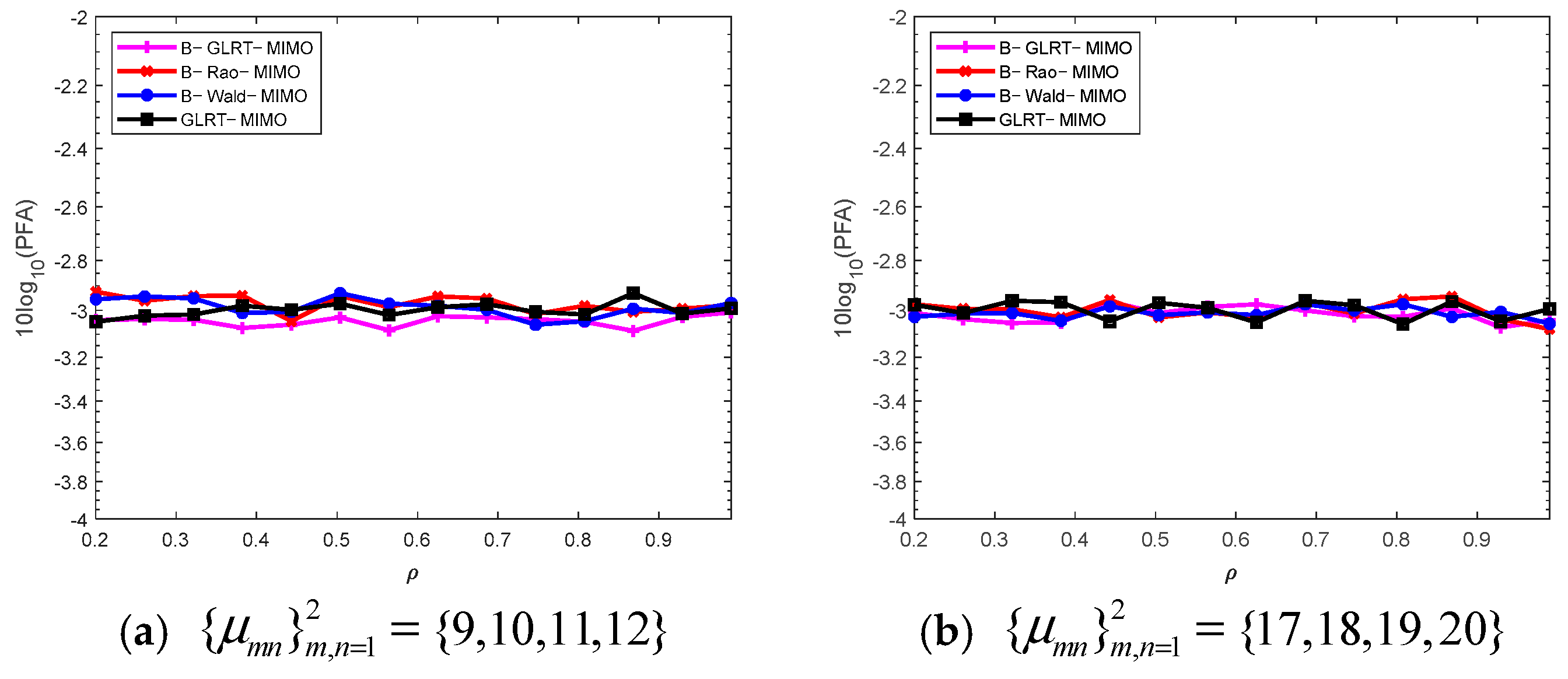
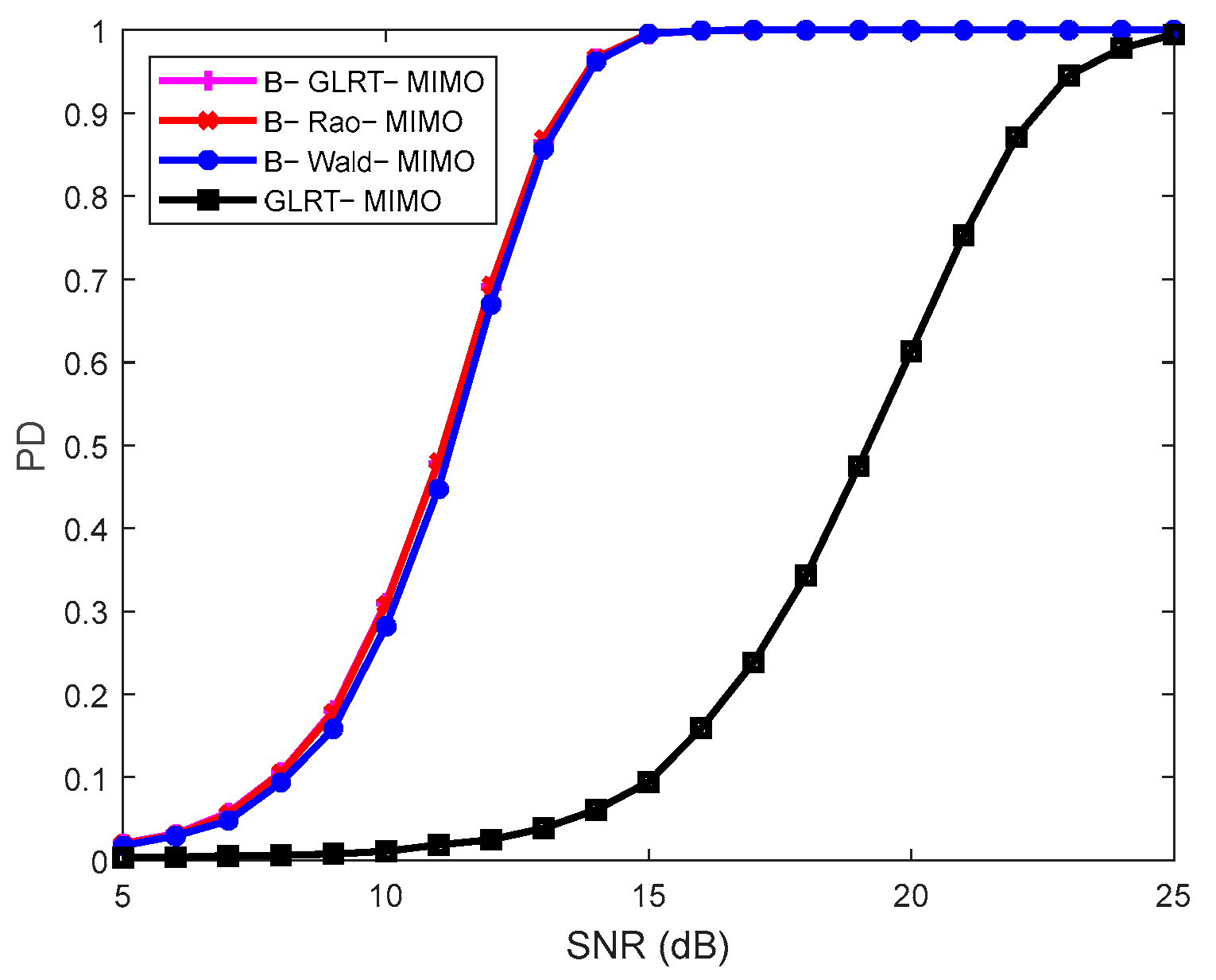
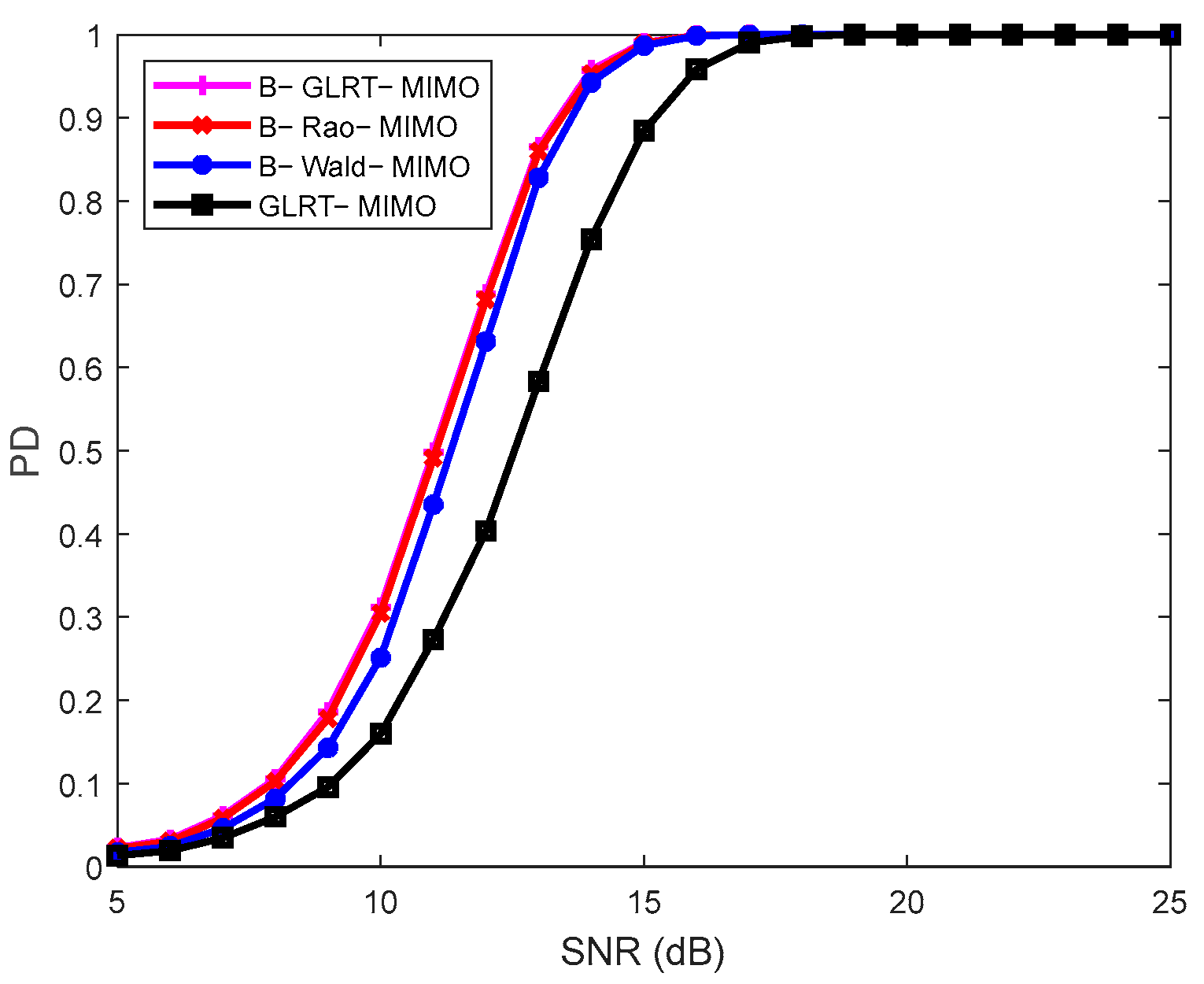
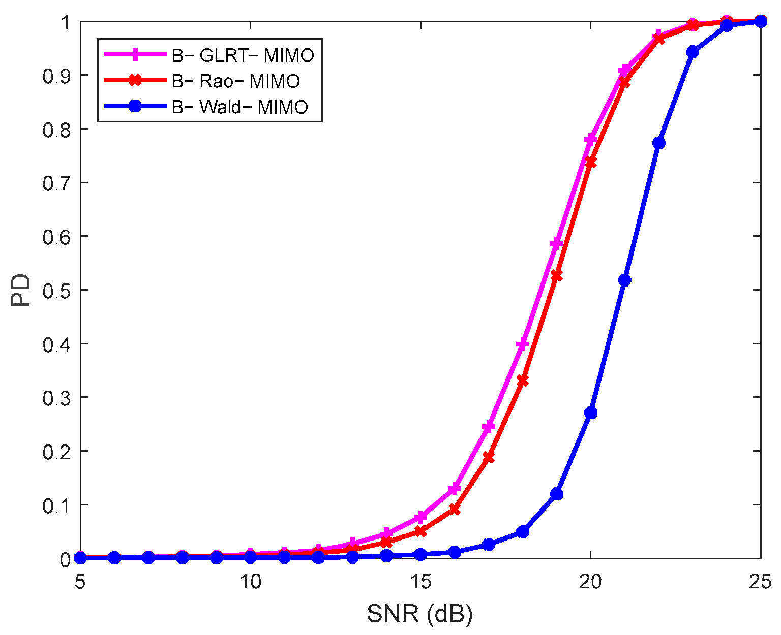
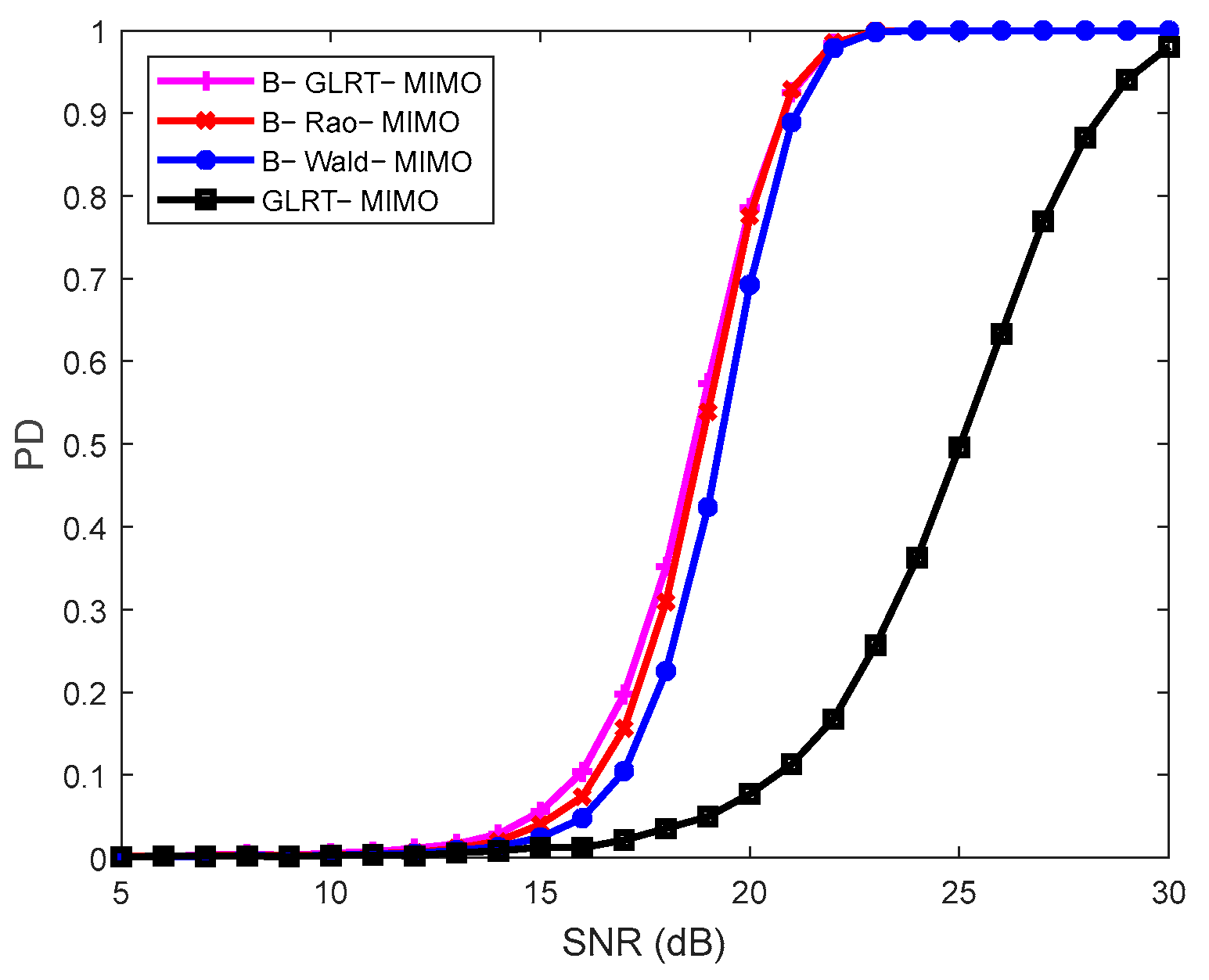
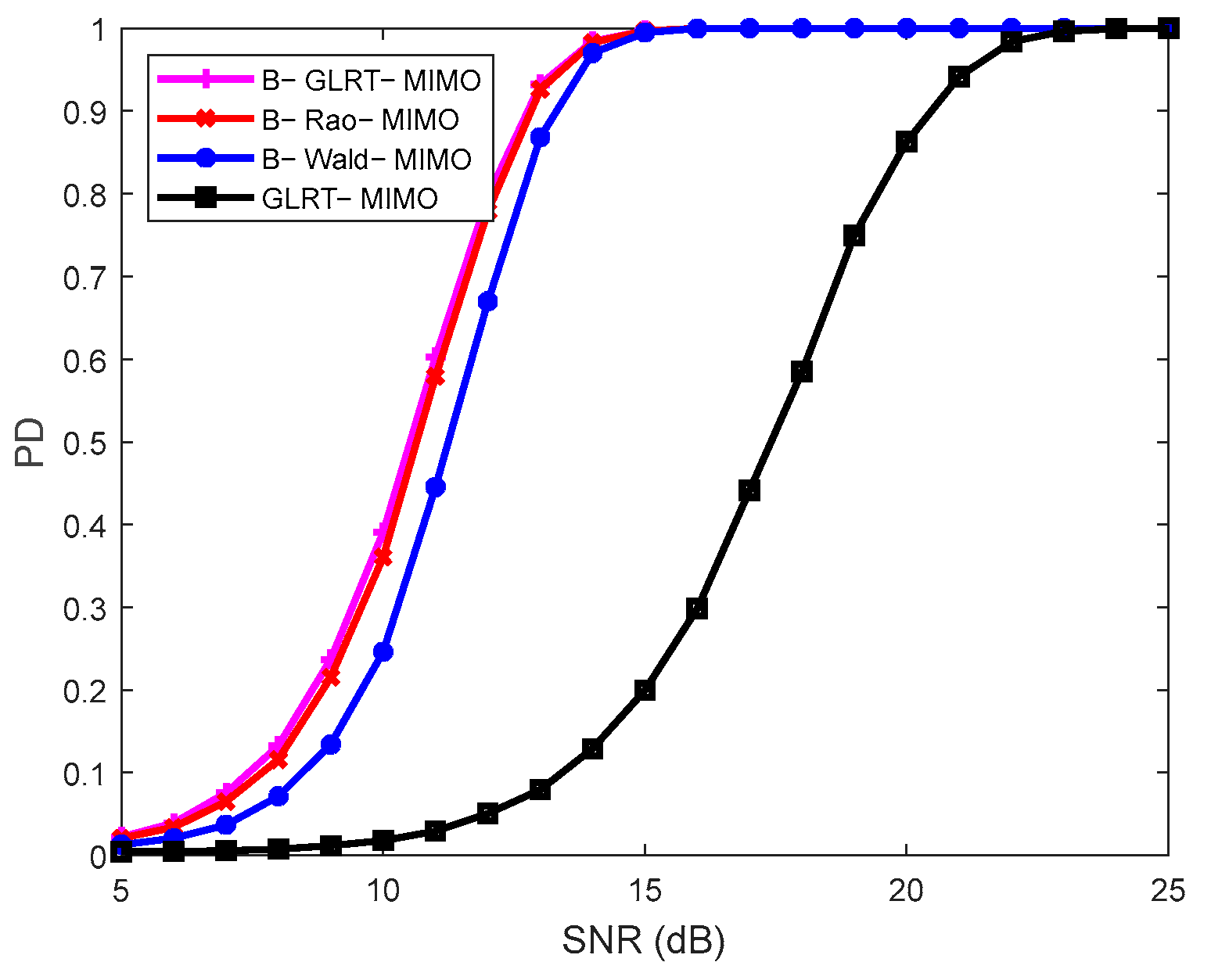
4. Performance Evaluation

This Section evaluates the detection performance of the proposed Bayesian detectors B-GLRT-MIMO, B-Rao-MIMO, and B-Wald-MIMO. To decrease the computational demands, the PFA is set to be $\mathrm{PFA}={10}^{-3}$. To determine the detection threshold, ${10}^5$ data simulations are used. To ascertain the probability of detection (PD), ${10}^4$ data simulations are conducted. The $(k_1,k_2)$ element of the Bayesian scalar matrix ${\mathsf{\Sigma }}_{mn}$ is set to be

$${\mathsf{\Sigma }}_{mn}(k_1,k_2)={\rho }_{mn}^{|k_1-k_2{|}^2}, k_1,k_2=1,2,\cdots ,K$$

(35)

The signal-to-noise ratio (SNR) is defined as

$$\mathrm{SNR}={\displaystyle \sum _{m=1}^M{\displaystyle \sum _{n=1}^N{\mathsf{\alpha }}_{mn}^H{H}_{mn}^H{\Sigma }_{mn}^{-1}{H}_{mn}{\mathsf{\alpha }}_{mn}}}$$

(36)

In order to verify the effectiveness of the proposed Bayesian MIMO radar detectors, this Section also presents the traditional subspace GLRT for the MIMO (GLRT-MIMO) radar, i.e.,

$$t_{\mathrm{GLRT}\text{-}\mathrm{MIMO}}={{\displaystyle \prod _{m=1}^M{\displaystyle \prod _{n=1}^N\left(\frac{1+x_{mn}^H{S}_{mn}^{-1}{x}_{mn}}{1+x_{mn}^H{S}_{mn}^{-1}{x}_{mn}-x_{mn}^H{S}_{mn}^{-1}{H}_{mn}{(H_{mn}^H{S}_{mn}^{-1}{H}_{mn})}^{-1}{H}_{mn}^H{S}_{mn}^{-1}{x}_{mn}}\right)}}}^{L_{mn}+1}$$

(37)

which is a subspace extension of the rank-one GLRT proposed in [19].

Figure 1 shows the probability of false alarms (PFAs) under different clutter covariance parameters ${\rho }_{mn}$ with a fixed detection threshold. For convenience, all ${\rho }_{mn}$ are set to be the same, i.e., ${\rho }_{11}={\rho }_{12}=\cdots ={\rho }_{MN}=\rho$. It can be seen from Figure 1 that the PFA remains basically constant, which verifies that the proposed detectors have the characteristic of constant false alarm rate (CFAR) properties.

Figure 2 shows the performance comparison between Bayesian detectors and the conventional GLRT-MIMO when the number of training samples is greater than the number of system channels. In this case, the number of transmitting antennas is $M=2$, the number of receiving antennas is $N=2$, the number of pulses within a CPI is $K=8$, and the Bayesian degrees of freedom are set to ${\left\{{\mu }_{mn}\right\}}_{m,n=1}^2=\{9,10,9,10\}$ for different transmitting-receiving antenna pairs. The values of ${\rho }_{mn}$ for the sale matrix in Equation (35) are ${\left\{{\rho }_{mn}\right\}}_{m,n=1}^2$ $=\{0.8,0.86,0.92,0.98\}$. The number of training samples is set to ${\left\{L_{mn}\right\}}_{m,n=1}^2=$$\{9,10,9,10\}$. For ease of writing, the above parameters are set as follows: Group 1 parameter settings. The dimension of the signal subspace is set to be $p=2$. From the results in Figure 2, it can be seen that the detection performance of the Bayesian MIMO radar detector is much higher than that of the conventional detector GLRT-MIMO. Among the three Bayesian detectors, the B-GLRT-MIMO has the highest PD. When the detection probability is 0.9, compared to the conventional detector GLRT-MIMO, the Bayesian MIMO radar detector B-GLRT-MIMO requires a reduction in SNR of more than 7 dB, which means an improvement in SNR of approximately 7 dB.

The parameters in Figure 3 are the same as those in Figure 2 except for the higher DOF of the inverse Wishart distribution. By comparing Figure 2 and Figure 3, it can be seen that when the DOF of the inverse Wishart distribution increases, the PD of each Bayesian detector increases. This is mainly due to the more accurate prior information about the unknown covariance matrix.

The parameters in Figure 4 are the same as those in Figure 2, except for the increase in the number of training samples. Compared with the results in Figure 2, it can be seen that the detection performance of each detector has improved, especially for the conventional detector GLRT-MIMO. However, it still has lower PD than the Bayesian detectors, and B-GLRT-MIMO also has the highest PD.

Figure 5 shows the PD of each Bayesian detector when the training samples are too limited to form an invertible SCM. Compared with the parameter settings in Figure 2, only the number of training samples is different. In this case, the conventional GLRT-MIMO fails, so it is not shown in the figure. It can be seen from Figure 5 that each Bayesian detector can effectively detect the target, and the detection performance of B-GLRT-MIMO is the best. Compared with Figure 2, the detection performance of each detector has decreased, mainly due to the insufficient number of training samples, which leads to a significant estimation error in the noise covariance matrix.

The parameters in Figure 6 are the same as those in Figure 2 except for the signal subspace dimension p. By comparing the results in Figure 2 and Figure 6, it can be seen that the increase in the dimension of the subspace will lead to a decrease in the PD of each detector. This is because the increase in the dimension of the subspace leads to an increase in the dimension of the unknown signal coordinates, and the increase in the number of unknowns will lead to a decrease in detection performance.

Figure 7 shows the detection performance of each detector when the receiving antenna is increased. Comparing the results of Figure 2 and Figure 7, it can be seen that the increase in the number of antennas in MIMO radar will lead to an improvement in detection performance. This seems reasonable, as more receiving antennas receive more reflected energy from the target, resulting in improved detection performance. However, the amount of equipment required for MIMO radar also increases at this time.

Table 1. Performance improvement of the Bayesian detectors w.r.t. the GLRT-MIMO at PD = 0.8.

Detector	Figure 2	Figure 3	Figure 4	Figure 5	Figure 6	Figure 7
B-GLRT-MIMO	7.21 dB	8.77 dB	1.72 dB	-	7.20 dB	7.43 dB
B-Rao-MIMO	7.02 dB	8.79 dB	1.68 dB	-	7.14 dB	7.31 dB
B-Wald-MIMO	6.42 dB	8.70 dB	1.49 dB	-	6.75 dB	6.79 dB

summarizes the performance gain of the Bayesian detectors compared to the conventional detector GLRT-MIMO in Figure 2, Figure 3, Figure 4, Figure 5, Figure 6 and Figure 7 at a PD of 0.8. The performance advantage of the Bayesian detectors can be intuitively seen from the table. Even when the training samples are sufficient, the proposed Bayesian detectors can still provide a performance gain of about 1.5 dB.

While enhancing the performance of radar target detection, the distributed MIMO system increases complexity due to the need for more antennas; the increase in data dimensions and data rates also raises the difficulty and time required for processing. The following strategies can be used to address or mitigate these issues:

• Optimized antenna design. Adopting advanced antenna technologies to reduce the physical size and complexity of the antennas without compromising performance. This may include the use of metamaterial-based antennas.
• Antenna selection techniques. Instead of using all available antennas, select a subset of antennas that offers the best trade-off between performance and complexity. This can reduce the number of antennas required and the associated system complexity.
• Compressed sensing. Utilizing compressed sensing techniques to reduce the amount of data that need to be processed. This method can effectively recover sparse signals from a small number of measurements.
• Parallel processing. Implementing parallel processing hardware, such as multi-core processors or field-programmable gate arrays (FPGAs), to handle the increased data processing demands. This can significantly reduce processing time.
• Algorithm optimization. Developing and implementing more efficient signal processing and data analysis algorithms. This may include algorithms specifically designed for processing high-dimensional data with lower computational complexity.
• Resource management. Implementing effective resource management strategies to efficiently allocate processing power and bandwidth. This helps optimize the use of available resources and reduces the overall system complexity.

5. Conclusions

This paper has successfully demonstrated the effectiveness of Bayesian theory in enhancing target detection performance in MIMO radar systems, particularly under conditions of insufficient training samples. By modeling the unknown covariance matrices as governed by inverse Wishart distributions and leveraging the GLRT, Rao, and Wald criteria, three Bayesian detectors were designed and evaluated. The results conclusively show that the proposed Bayesian detectors have CFAR properties and outperform conventional detectors, with the B-GLRT-MIMO detector exhibiting the highest PD. Remarkably, the B-GLRT-MIMO enhances performance by over 7 dB in SNR, compared with the existing detection method. Furthermore, the proposed Bayesian detectors are capable of functioning effectively even in the absence of training data. The study highlights the importance of prior information accuracy in improving detection performance, as evidenced by the increased PD with higher degrees of freedom for the inverse Wishart distribution. Additionally, increasing the number of receiving antennas in MIMO radar systems enhances detection capabilities, albeit with a corresponding increase in hardware complexity. Overall, this work provides a robust framework for addressing the challenges of target detection in MIMO radar with limited training data, offering valuable insights for future research and practical applications.

References

1. Liu, W.; Liu, J.; Hao, C.; Gao, Y.; Wang, Y.-L. Multichannel adaptive signal detection: Basic theory and literature review. Sci. China Inf. Sci. 2022, 65, 121301. [Google Scholar] [CrossRef]
2. Shen, W.; Wang, S.; Wang, Y.; Li, Y.; Lin, Y.; Zhou, Y.; Xu, X. Moving Target Detection Algorithm for Millimeter Wave Radar Based on Keystone-2DFFT. Electronics 2023, 12, 4776. [Google Scholar] [CrossRef]
3. Yang, C.; Wang, X.; Ni, W. Joint Transmit and Receive Beamforming Design for DPC-Based MIMO DFRC Systems. Electronics 2024, 13, 1846. [Google Scholar] [CrossRef]
4. Liu, Y.; Pan, C.; Liu, X.; Zhu, Y.; Liu, Y. A Waveform Design for MIMO Sensing on Two-Dimensional Arrays with Sparse Estimation. Electronics 2023, 12, 3906. [Google Scholar] [CrossRef]
5. Zaimbashi, A.; Li, J. Tunable Adaptive Target Detection With Kernels in Colocated MIMO Radar. IEEE Trans. Signal Process. 2020, 68, 1500–1514. [Google Scholar] [CrossRef]
6. Liu, W.; Wang, Y.-L.; Liu, J.; Xie, W.; Chen, H.; Gu, W. Adaptive Detection Without Training Data in Colocated MIMO Radar. IEEE Trans. Aerosp. Electron. Syst. 2015, 51, 2469–2479. [Google Scholar] [CrossRef]
7. Pan, X.; Li, S.; Pan, C. Distributed broadband phased-MIMO sonar for detection of small targets in shallow water environments. IET Radar Sonar Navig. 2018, 12, 721–728. [Google Scholar] [CrossRef]
8. Yang, S.; Yi, W.; Jakobsson, A. Multitarget Detection Strategy for Distributed MIMO Radar With Widely Separated Antennas. IEEE Trans. Geosci. Remote Sens. 2022, 60, 1–16. [Google Scholar] [CrossRef]
9. Li, J.; Stoica, P. MIMO radar with colocated antennas. IEEE Signal Process. Mag. 2007, 24, 106–114. [Google Scholar] [CrossRef]
10. Haimovich, A.M.; Blum, R.S.; Cimini, L.J. MIMO radar with widely separated antennas. IEEE Signal Process. Mag. 2008, 25, 116–129. [Google Scholar] [CrossRef]
11. He, C.; Zhang, R.; Huang, B.; Xu, M.; Wang, Z.; Liu, L.; Lu, Z.; Jin, Y. Moving-Target Detection for FDA-MIMO Radar in Partially Homogeneous Environments. Electronics 2024, 13, 851. [Google Scholar] [CrossRef]
12. Shikhaliev, A.P.; Himed, B. Distributed MIMO Radar Adaptive Detection in the Presence of Spectral Symmetry. IEEE Trans. Aerosp. Electron. Syst. 2023, 59, 4721–4728. [Google Scholar] [CrossRef]
13. Zaimbashi, A.; Greco, M.S.; Gini, F. Distributed MIMO Passive Radar Target Detection: Holy Trinity, Durbin, and Gradient Tests. IEEE Trans. Aerosp. Electron. Syst. 2024, 60, 3427–3441. [Google Scholar] [CrossRef]
14. Jing, X.; Su, H.; Jia, C.; Mao, Z.; Shen, L. Fusion detection in distributed MIMO radar under hybrid-order Gaussian model. Signal Process. 2024, 214, 109256. [Google Scholar] [CrossRef]
15. Fishler, E.; Haimovich, A.; Blum, R.S.; Leonard, J.; Cimini, J.; Chizhik, D.; Valenzuela, R.A. Spatial Diversity in Radars—Models and Detection Performance. IEEE Trans. Signal Process. 2006, 54, 823–838. [Google Scholar] [CrossRef]
16. De Maio, A.; Lops, M. Design principles of MIMO radar detectors. IEEE Trans. Aerosp. Electron. Syst. 2007, 43, 886–898. [Google Scholar] [CrossRef]
17. De Maio, A.; Lops, M.; Venturino, L. Diversity-integration tradeoffs in MIMO detection. IEEE Trans. Signal Process. 2008, 56, 5051–5061. [Google Scholar] [CrossRef]
18. Sheikhi, A.; Zamani, A. Temporal coherent adaptive target detection for multi-input multi-output radars in clutter. IET Radar Sonar Navig. 2008, 2, 86–96. [Google Scholar] [CrossRef]
19. Liu, J.; Zhang, Z.J.; Cao, Y.H.; Yang, S.Y. A closed-form expression for false alarm rate of adaptive MIMO-GLRT detector with distributed MIMO radar. Signal Process. 2013, 93, 2771–2776. [Google Scholar] [CrossRef]
20. Hu, Q.; Su, H.; Zhou, S.; Liu, Z.; Yang, Y.; Liu, J. Two-stage constant false alarm rate detection for distributed multiple-input–multiple-output radar. IET Radar Sonar Navig. 2016, 10, 264–271. [Google Scholar] [CrossRef]
21. Chen, P.; Zheng, L.; Wang, X.; Li, H.; Wu, L. Moving Target Detection Using Colocated MIMO Radar on Multiple Distributed Moving Platforms. IEEE Trans. Signal Process. 2017, 65, 4670–4683. [Google Scholar] [CrossRef]
22. Zhu, L.; Wen, G.; Liang, Y.; Luo, D.; Song, H. Parametric Wald test for target detection with distributed MIMO radar in partially mixing homogeneous and non-homogeneous environments. IET Radar Sonar Navig. 2022, 16, 470–486. [Google Scholar] [CrossRef]
23. Zeng, C.; Wang, F.; Li, H.; Govoni, M.A. Target Detection for Distributed MIMO Radar With Nonorthogonal Waveforms in Cluttered Environments. IEEE Trans. Aerosp. Electron. Syst. 2023, 59, 5448–5459. [Google Scholar]
24. Wang, P.; Li, H.B.; Himed, B. Moving Target Detection Using Distributed MIMO Radar in Clutter With Nonhomogeneous Power. IEEE Trans. Signal Process. 2011, 59, 4809–4820. [Google Scholar] [CrossRef]
25. Li, H.; Wang, Z.; Liu, J.; Himed, B. Moving Target Detection in Distributed MIMO Radar on Moving Platforms. IEEE J. Sel. Top. Signal Process. 2015, 9, 1524–1535. [Google Scholar] [CrossRef]
26. Gao, Y.; Li, H.; Himed, B. Knowledge-Aided Range-Spread Target Detection for Distributed MIMO Radar in Nonhomogeneous Environments. IEEE Trans. Signal Process. 2017, 65, 617–627. [Google Scholar] [CrossRef]
27. Maio, A.D.; Farina, A.; Foglia, G. Knowledge-Aided Bayesian Radar Detectors & Their Application to Live Data. IEEE Trans. Aerosp. Electron. Syst. 2010, 46, 170–183. [Google Scholar]
28. Tague, J.A.; Caldwell, C.I. Expectations of useful complex Wishart forms. Multidimens. Syst. Signal Process. 1994, 5, 263–279. [Google Scholar] [CrossRef]
29. Liu, W.; Wang, Y.-L.; Xie, W. Fisher Information Matrix, Rao Test, and Wald Test for Complex-Valued Signals and Their Applications. Signal Process. 2014, 94, 1–5. [Google Scholar] [CrossRef]
30. Sun, M.; Liu, W.; Liu, J.; Hao, C. Complex parameter Rao, Wald, gradient, and Durbin tests for multichannel signal detection. IEEE Trans. Signal Process. 2022, 70, 117–131. [Google Scholar] [CrossRef]
Figure 1. PFAs of the detectors under different clutter structure. M = 2 , N = 2 , K = 8 , { L m n } m , n = 1 2 = { 9 , 10 , 9 , 10 } , and p = 2 .
Electronics 14 00164 g001
Figure 2. PDs of the detectors under different SNRs. M = 2 , N = 2 , K = 8 , { μ m n } m , n = 1 2 =   { 9 , 10 , 11 , 12 } , { ρ m n } m , n = 1 2 = { 0.8 , 0.86 , 0.92 , 0.98 } , { L m n } m , n = 1 2 = { 9 , 10 , 9 , 10 } , and p = 2 .
Electronics 14 00164 g002
Figure 3. PDs of the detectors under different SNRs. M = 2 , N = 2 , K = 8 , { μ m n } m , n = 1 2 =   { 17 , 18 , 19 , 20 } , { ρ m n } m , n = 1 2 = { 0.8 , 0.86 , 0.92 , 0.98 } , { L m n } m , n = 1 2 = { 9 , 10 , 9 , 10 } , and p = 2 .
Electronics 14 00164 g003
Figure 4. PDs of the detectors under different SNRs. M = 2 , N = 2 , K = 8 , { μ m n } m , n = 1 2 =   { 9 , 10 , 11 , 12 } , { ρ m n } m , n = 1 2 = { 0.8 , 0.86 , 0.92 , 0.98 } , { L m n } m , n = 1 2 = { 15 , 16 , 15 , 16 } , and p = 2 .
Electronics 14 00164 g004
Figure 5. PDs of the detectors under different SNRs. M = 2 , N = 2 , K = 8 , { μ m n } m , n = 1 2 =   { 9 , 10 , 11 , 12 } , { ρ m n } m , n = 1 2 = { 0.8 , 0.86 , 0.92 , 0.98 } , { L m n } m , n = 1 2 = { 4 , 5 , 4 , 5 } , and p = 2 .
Electronics 14 00164 g005
Figure 6. PDs of the detectors under different SNRs. M = 2 , N = 2 , K = 8 , { μ m n } m , n = 1 2 =   { 9 , 10 , 11 , 12 } , { ρ m n } m , n = 1 2 = { 0.8 , 0.86 , 0.92 , 0.98 } , { L m n } m , n = 1 2 = { 9 , 10 , 9 , 10 } , and p = 6 .
Electronics 14 00164 g006
Figure 7. PDs of the detectors under different SNRs. M = 2 , N = 3 , K = 8 , { μ m n } m , n = 1 2 =   { 9 , 10 , 11 , 12 , 13 , 14 } , { ρ m n } m , n = 1 2 = { 0.8 , 0.836 , 0.872 , 0.908 , 0.98 } , { L m n } m , n = 1 2 = { 9 , 10 , 9 , 10 , 9 , 10 } , and p = 2 .
Electronics 14 00164 g007