Heterogeneous Multi-Agent Risk-Aware Graph Encoder with Continuous Parameterized Decoder for Autonomous Driving Trajectory Prediction

Abstract

Trajectory prediction is a critical component of autonomous driving, intelligent transportation systems, and human–robot interactions, particularly in complex environments like intersections, where diverse road constraints and multi-agent interactions significantly increase the risk of collisions. To address these challenges, a Heterogeneous Risk-Aware Graph Encoder with Continuous Parameterized Decoder for Trajectory Prediction (HRGC) is proposed. The architecture integrates a heterogeneous risk-aware local graph attention encoder, a low-rank temporal transformer, a fusion lane and global interaction encoder layer, and a continuous parameterized decoder. First, a heterogeneous risk-aware edge-enhanced local attention encoder is proposed, which enhances edge features using risk metrics, constructs graph structures through graph optimization and spectral clustering, maps these enhanced edge features to corresponding graph structure indices, and enriches node features with local agent-to-agent attention. Risk-aware edge attention is aggregated to update node features, capturing spatial and collision-aware representations, embedding crucial risk information into agents’ features. Next, the low-rank temporal transformer is employed to reduce computational complexity while preserving accuracy. By modeling agent-to-lane relationships, it captures critical map context, enhancing the understanding of agent behavior. Global interaction further refines node-to-node interactions via attention mechanisms, integrating risk and spatial information for improved trajectory encoding. Finally, a trajectory decoder utilizes the aforementioned encoder to generate control points for continuous parameterized curves. These control points are multiplied by dynamically adjusted basis functions, which are determined by an adaptive knot vector that adjusts based on velocity and curvature. This mechanism ensures precise local control and the superior handling of sharp turns and speed variations, resulting in more accurate real-time predictions in complex scenarios. The HRGC network achieves superior performance on the Argoverse 1 benchmark, outperforming state-of-the-art methods in complex urban intersections.

1. Introduction

Autonomous driving has increasingly garnered widespread attention. An autonomous driving system consists of perception/localization, prediction, planning, and control modules [1,2,3]. The perception/localization module captures raw sensor data and constructs HD maps. The output of this process includes historical trajectories, representing the positions and states of agents, as well as lane scene information, which serve as unstructured data inputs for trajectory prediction. Accurate and reliable trajectory prediction of road agents, such as cars and pedestrians, is crucial for decision making and safety in autonomous driving systems. However, in complex environments like intersections, conventional pipelines often overlook the collision risks arising from multi-agent interactions. How can we effectively model heterogeneous multi-agent interactions while integrating risk reasoning?

The nature of trajectory prediction data is inherently heterogeneous, encompassing various elements such as agents’ motion states, traffic lights with positions, lane polylines representing feasible movement paths, and road line polygons of different types. Recent advancements have highlighted the potential of exploiting the heterogeneity within driving scenes. Trajectron++ [4] and HEAT [5] encode different types of agents with different parameters, but they encode map elements using rasterized representation, which leads to inferior performance compared to vector-based methods [6]. VectorNet-based approaches [6,7,8] put all agents and lanes in one single fully connected graph and use shared parameters for information aggregation, which ignores different node types and semantic relations. LaneGCN-based [9] solutions [10,11,12] introduce a series of four graphs (lane to agent, lane to lane, lane to actor and lane to actor) according to the distance heuristics and connective information of the lane. Recent advancements in heterogeneous graph-based trajectory prediction, such as HDGT [13] and HIVT [14], have effectively modeled interactions between diverse traffic agents and road elements. However, these methods typically do not incorporate risk reasoning into the prediction process. While works like HTF [15] and DRM-DL [16] have introduced risk metrics, focusing on collision probabilities and maneuvering intentions, they lack the ability to embed the heterogeneous features of multi-agent relationships. As shown in Figure 1, our method integrates risk assessment into a heterogeneous graph framework, encoding complex risk-based collision metrics among agents to capture dynamic traffic interactions. This enables our approach to achieve more accurate and robust trajectory predictions by effectively modeling the inter-agent risk dynamics.

Modeling uncertainty is a critical aspect of trajectory prediction for ensuring accuracy and robustness. Methods like Gaussian Mixture Models (e.g., Multipath++ [17] and MTR [18]) and Laplacian distribution-based models (e.g., HIVT [14]) explicitly model trajectory probability distributions, enabling uncertainty-aware predictions. Other approaches, such as HEAT [5], utilize sequential models like LSTMs to capture temporal dependencies, while methods like LaneRCNN [10] and SIMPL [19] employ continuous parameterized curves (e.g., Bezier curves) for smooth trajectory generation. However, these methods often face challenges in handling dynamic scenarios with significant speed changes like a complete stop. To address this challenges, we propose a novel trajectory decoder using B-splines, which dynamically adapts to speed and curvature variations, offering robust predictions in complex environments.

To address the challenges of risk-aware trajectory prediction in complex driving scenarios, we propose a novel architecture that integrates a heterogeneous risk-aware graph encoder, a low-rank temporal transformer, and a continuous parameterized decoder. These components work together to model complex multi-agent interactions, capture temporal dependencies, and generate smooth, adaptable trajectories. The risk-aware graph encoder captures agent-to-agent interactions and collision risks in dense scenarios. The low-rank temporal transformer reduces computational complexity while maintaining accuracy in dynamic environments. Finally, the continuous parameterized decoder, with its adaptive knot vector mechanism, dynamically adjusts trajectories based on velocity and curvature, ensuring precision in scenarios like sharp turns and stop-and-go motions.

Toward a practical multi-agent trajectory prediction engine for autonomous driving, the main contributions are as follows:

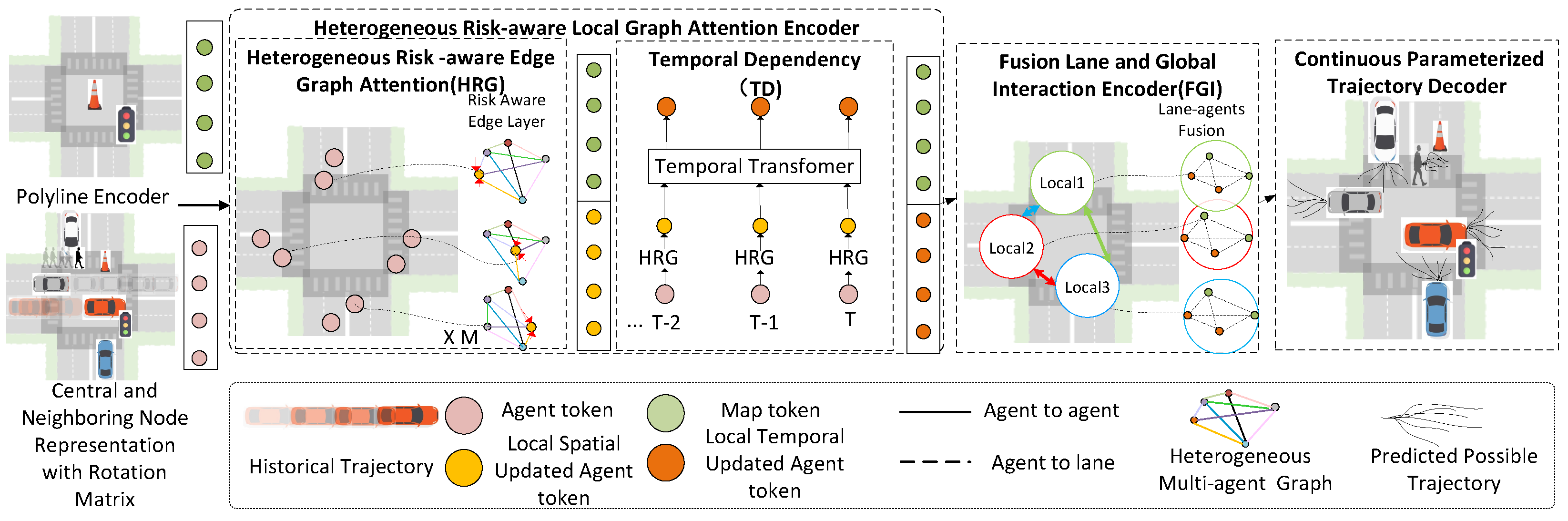
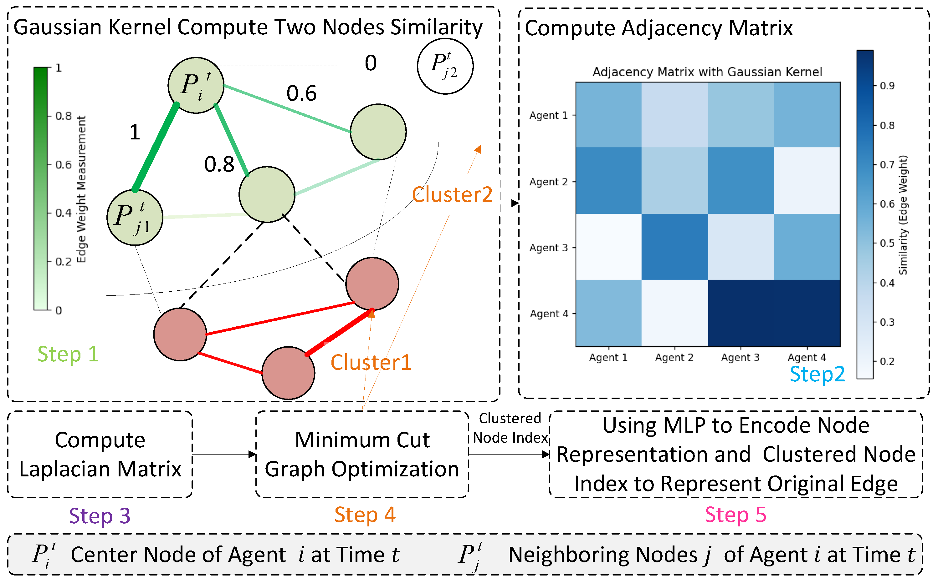
• Heterogeneous Multi-agent Risk-aware Graph Attention Encoder: By computing agent risk assessment attributes and map these features to a graph structure, the graph built by graph optimization and clustering method. These edge and node features are then processed through a node attention mechanism to model complex agent interactions, enhancing trajectory prediction accuracy and robustness.
• Low-Rank Temporal Transformer: We introduced a low-rank temporal transformer layer to reduce computational complexity and maintain accuracy, improving robustness in dynamic environments.
• Continuous Parameterized Trajectory Prediction Decoder: We proposed a continuous parameterized trajectory decoder, generating control points influenced by an adaptive knot vector, enabling precise trajectory predictions and handling sudden motion changes effectively.

2. Related Works

2.1. Homogeneous Graph Interaction in Trajectory Prediction

Graphs, as a widely used structure, consist of nodes and edges. Nodes typically represent entities or elements, while edges denote relationships between connected nodes. To represent the structure and information within a graph, Graph Neural Networks [20] were introduced, which generally comprise two main functions: an aggregation function and an update function. The aggregation function focuses on gathering features from neighboring nodes, summarizing the context for the current node. The update function generates new representations for each node based on the aggregated neighbor information and the node’s original features, enabling the node to better reflect its role and state within the overall graph. Two of the most widely used GNN models are the GCN [20], which utilizes the graph’s Laplacian matrix, and the GAT [21], which applies attention mechanisms for aggregation and updating.

Heterogeneous graphs contain multiple types of entities (nodes) and relationships (edges). HGN [22] utilizes node-level and semantic-level attention, based on the GAT [21], to learn relationships between nodes and their meta-path neighbors, thereby generating more interpretable and superior-performing node embeddings in heterogeneous graphs. On the other hand, HetSANN [23], a novel heterogeneous graph structural attention neural network, leverages the GCN [20] to directly encode the structural information of heterogeneous information networks without relying on meta-paths, thus automatically processing heterogeneous information. In the context of trajectory prediction within a driving scene, a heterogeneous graph can represent different entities as nodes, such as agents (vehicles, pedestrians, cyclists, etc.) or map elements (lanes, traffic lights, stop signs, etc.). Each node typically holds specific information, known as node features, which may include the agent’s state (position or velocity), lane type, or the polyline that represents its geometry.

One edge usually contains information (called an edge feature), e.g., the relative position between two entities or relations (Lane, Left Lane, Agent Lane, etc.). Trajectron++ [4] encodes different types of agents with different parameters of GNNs. HEAT [5] proposes a Heterogeneous Edge-Enhanced Graph Attention Network to extract the historical dynamics of different types of agents and interactions between agents through a directed heterogeneous graph, enabling multi-agent trajectory prediction in complex traffic scenarios. However, as pioneering works, they encode the map elements using rasterized images and use a CNN to extract the representation vectors of maps. According to the recent progress in the trajectory prediction community, this approach is inefficient and leads to much inferior performance compared to vector-based methods [6]. VectorNet [6] introduces a hierarchical graph neural network that uses vector representations of road components and agent trajectories to model interactions, reducing computational complexity compared to rendering-based approaches. TPCN [24] combines point cloud learning with dynamic temporal learning to jointly capture spatial and temporal information for trajectory prediction.

In recent heterogeneous graph-based trajectory prediction models, Graphad [25] introduces an Interaction Scene Graph to efficiently model heterogeneous interactions among the ego vehicle, road agents, and map elements, improving performance in perception, prediction, and planning for autonomous driving. Diffusion models have emerged as a promising approach, particularly in temporal prediction tasks. This enables them to better handle the uncertainty inherent in long-term trajectory forecasting. The core idea of Linformer [26] is to approximate the self-attention matrix as a low-rank matrix, utilizing linear projections to reduce its dimensionality. This approach decreases the complexity from O(n²) to O(n), significantly enhancing memory and time efficiency while maintaining model performance. Inspired by the Linformer architecture, we design a low-rank temporal transformer that reduces computational complexity while maintaining accuracy.

2.2. Risk Assessment in Trajectory Forecasting

In complex driving situations, collision avoidance is a crucial component of system safety, which requires a comprehensive analysis of collision risk. Driving risk can mainly be assessed through five methods [27]: time-based metrics, statistics-based metrics, field-based metrics, kinematics-based metrics, and unexpected driving behavior-based metrics. The simplest and most efficient approach is time-based metrics, such as Time-to-Collision (TTC) techniques [28,29], which measure the time remaining until a collision would occur if two vehicles maintain their current speeds. TTC has been widely adopted for evaluating driving risks, particularly in collision warning and avoidance systems. Recently, Wang et al. [30] proposed a two-stage multi-modal trajectory prediction model to assess driving risk on highways by combining lane-change predictions and potential collision risks. Fang et al. [15] using a Heterogeneous Risk Graph and a Hierarchical Scene Graph to model interactions between agents and their environment, leveraging collision risk metrics and road scene semantics for accurate predictions. Both approaches align with risk-based trajectory forecasting methods that utilize the TTC-based approach. In our method, we also use TTC within edge to be a novel risk-aware edge for graph message passing. The concept of “Collaborative Uncertainty” (CU) is employed to capture the uncertainty arising from multi-agent interactions for trajectory prediction, such as interaction collaborative uncertainty [31]. Additionally, methods that combine trajectory distribution uncertainty and driving intention uncertainty are applied. DRM-DL [16] proposes a method that integrates driving risk uncertainty and trajectory distribution uncertainty into a deep learning framework to improve the accuracy of interactive multi-vehicle trajectory prediction. Similarly, we construct one heterogeneous graph, including both agents, map elements, and an risk-aware edge aggregate, into the node update attention structure of the heterogeneous graph.

2.3. Trajectory Representation for Trajectory Forecasting

For the trajectory prediction decoder, trajectory representation is a key problem. In terms of modeling uncertainty, some methods model the trajectory’s probability distribution to define uncertainty. Gaussian Mixture Model (GMM): Multipath++ [17] utilizes the GMM to model trajectories, selecting optimal trajectory centroids through a clustering algorithm and refining them using the Expectation–Maximization (EM) algorithm. Similarly, MTR [18] employs the GMM but places greater emphasis on probability distribution modeling and centroid extraction, focusing on generating trajectories through these distributions. Laplacian Distribution: HIVT [14] leverages a Laplace distribution, where the position parameter represents the location, and the scale parameter encodes uncertainty. HIVT predicts trajectory distribution parameters, including position and uncertainty, using an MLP, which is further combined with softmax to generate mixing coefficients. However, MTR directly predicts the trajectory distribution parameters, such as the mean and covariance matrix, without requiring an explicit decoder for additional uncertainty prediction. Direct Trajectory Coordinate Prediction: Unlike probability distribution-based methods that explicitly model uncertainty and output trajectory distribution parameters (e.g., mean and variance/scale), HDGT [13] adopts an MLP to directly predict trajectory coordinates along with confidence scores for each mode. This approach does not assume an explicit probability distribution but instead selects the optimal mode by minimizing the coordinate error. Sequential Temporal Modeling: HEAT [5] employs Long Short-Term Memory (LSTM), which is a sequential model adept at capturing both short-term and long-term dependencies in time-series data, making it highly suitable for trajectory prediction. LSTM takes as input individual dynamic features, interaction features, and map features concatenated together. It predicts the position for the next H time steps, with each time step’s state updated based on the previous state and the current input features. A fully connected layer maps the hidden state at each time step to the specific physical attributes of the trajectory, such as position. While effective, LSTM outputs often require an MLP to convert them into specific trajectory prediction results. Parameterized Curve-Based Decoders: After aggregating encoder feature tokens, sequential temporal changes can be modeled using transformer architectures [14] or LSTMs. Typically, an MLP with a regression head is employed for trajectory prediction alongside a classification head with softmax to compute probability scores. Rather than directly predicting future trajectory positions, methods like LaneRCNN [10], SIMPL [19], and HTF [15] adopt a continuous parameterized representation for trajectory regression. These methods often rely on Bezier curves, which offer a continuous representation with smooth motion and precise higher-order derivatives.

However, Bezier curves have inherent limitations due to their fixed control points and degree, which restrict their flexibility in handling dynamic scenarios with significant speed variations. While the “hodograph property” of Bezier curves allows for direct derivative computation, numerical imbalances in coefficients can lead to reduced trajectory prediction accuracy, making them less suitable for complex and highly dynamic environments. In autonomous driving scenarios, agents often experience dynamic changes in speed, such as coming to a complete stop or sudden acceleration. To address this, our method employs B-splines, which allow for non-uniform parameterization using a dynamically adjusted knot vector. It enables the model to adapt to changes in speed and curvature, providing more robust trajectory predictions in complex environments.

3. Methods

3.1. Problem Formulation and Approach Overview

We address the task of predicting future trajectories of dynamic agents based on their historical states and the context of the map. The input consists of the agents’ past states, including their position, velocity, heading, and type (e.g., pedestrian, cyclist, vehicle), along with surrounding map elements such as lanes, traffic lights, and other key road features. Our goal is to forecast future trajectories over the next T time steps, providing multiple predictions to account for inherent uncertainty.

Our HRGC trajectory predictor leverages heterogeneous graph representations to effectively capture complex interactions between agents and map elements. We propose a risk-aware edge mechanism that models agent interactions with greater precision, incorporating factors like time to collision for more accurate predictions. Furthermore, we design a continuous parameterized trajectory decoder that derives control points from encoder-extracted features, combining them with basis functions influenced by an adaptive knot vector. By dynamically adjusting the knot vector based on velocity and curvature, our method delivers precise trajectory generation, allowing it to seamlessly handle sharp turns and sudden speed variations.

The pipeline of our method HRGC trajectory predictor is shown in Figure 2, which involves the following:

• Section 3.2: Central and neighboring node representation.
• Section 3.3: Heterogeneous risk-aware local graph attention encoder with low-rank temporal transformer.
• Section 3.4: Fusion lane and global interaction encoder.
• Section 3.5: Continuous parameterized trajectory prediction decoder.

3.2. Central and Neighboring Node Representation

To exploit the symmetries of the problem, we use the rotation transformation for each agent. Specifically, we uniformly take the central agent $i^{\prime }s$ embedding ${\mathbf{C}}_i^t\in {\mathbb{R}}^{d_h}$ and any neighboring agent $j^{\prime }s$ embedding ${\mathbf{C}}_{ij}^t\in {\mathbb{R}}^{d_h}$ at any time step t:

$${\mathbf{z}}_i^t=ML{P}_{\mathrm{center}}\left(\left[\begin{array}{c}{\mathbf{R}}_i^{\top }\left({\mathbf{p}}_i^t-{\mathbf{p}}_i^{t-1}\right),V{m}_i^t,V{a}_i^t\end{array}\right]\right),$$

(1)

$${\mathbf{z}}_{ij}^t=ML{P}_{\mathrm{nbr}}\left(\left[{\mathbf{R}}_i^{\top }\left({\mathbf{p}}_j^t-{\mathbf{p}}_j^{t-1}\right),{\mathbf{R}}_i^{\top }\left({\mathbf{p}}_j^t-{\mathbf{p}}_i^t\right),V{m}_j^t,V{a}_j^t\right]\right),$$

(2)

where $ML{P}_{\mathrm{center}}$ and $ML{P}_{\mathrm{nbr}}$ are two different MLP blocks, ${\mathbf{R}}_i\in {\mathbb{R}}^{2\times 2}$ is the rotation matrix parameterized by ${\theta }_i$, $V{m}_i^t,V{a}_i^t$ and $V{m}_j^t,V{a}_j^t$ are the velocity magnitude and velocity angle of agent i and j, respectively. Since all geometric attributes are normarlized with respect to the central agent before they are fed into MLPs, these embeddings are unaffected by the rotation of the global coordinate frame. Apart from the trajectory segments, the inputs of $ML{P}_{\mathrm{nbr}}$ also contain neighboring agents’ position vectors relative to the central agent, making the neighboring embedding spatially aware.

3.3. Heterogeneous Risk-Aware Local Graph Attention Encoder

In multi-agent interaction scenarios, understanding the dynamic relationships among various agents is vital for safe driving and accurate prediction in complex environments. The heterogeneous risk-aware local graph utilizes an edge-based attention mechanism.

After transforming the center and neighboring nodes, edge features are built, and the TTC and moving direction with velocity risk between nodes are computed. Then, a Gaussian kernel is used to calculate the similarity between nodes, followed by the computation of the Laplacian matrix and degree matrix. The Laplacian matrix is normalized, and clustering methods, along with a minimum graph optimization, are applied to obtain the cluster edge index. Finally, the computed risk-aware features are mapped to the corresponding index.

Our attention can capture the interaction relationship between different agents while taking into account the potential collision risk. In contrast, recent studies only considered the physical or geometrical relationship. This collision risk metric, such as time to collision, takes into account the road type (intersection, walking, vehicle, etc.) and moving direction with velocity. This enables us to effectively capture these complex relationships and more accurately compute the collision risk.

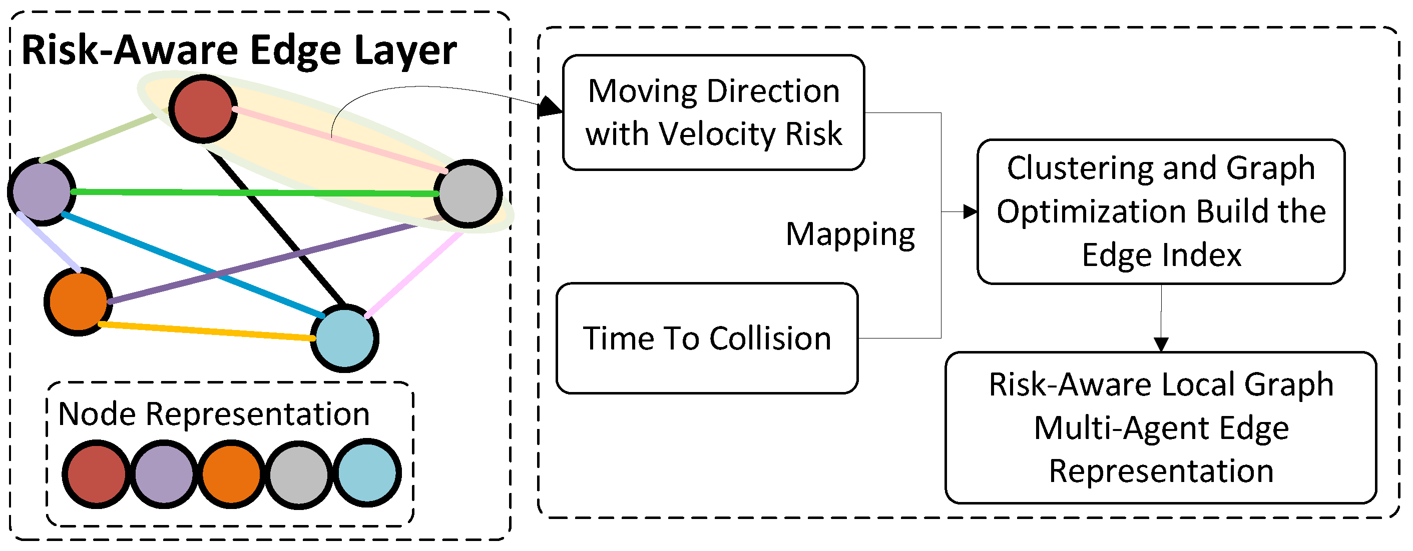
3.3.1. Risk-Aware Edge Layer

In Figure 3, we propose risk-aware edge layer, which is similar to the transformation from a dense graph to a sparse graph. In this process, we first compute the node similarities using a Gaussian kernel, and then construct the normalized Laplacian matrix and degree matrix. Clustering and graph optimization methods are applied to obtain the edge indices. The edge features, computed from the TTC and moving direction with velocity risk, are then mapped back to the corresponding indices. It not only captures spatial relationships but also takes into account their movement trends, improving the ability to model collision risks.

The risk-aware edge calculation between agents i and j can be formulated as follows:

$$e_t^{ij}=O_t^{ij}·{\displaystyle \frac{1}{|T_t^{ij}|}}·m_t^{ij},\mathrm{s}.\mathrm{t}.,s_t^i,s_t^j\in S_t$$

(3)

where $e_t^{ij}$ represents the edge feature between node i and node j at time t. It quantifies the interaction risk between the two nodes by incorporating factors such as their movement direction, velocity, and time to collision. $O_t^{ij}$ denotes the velocity risk between node i and node j based on direction similarity and velocity differences. $T_t^{ij}$ represents time to collision between node i and j. $m_t^{ij}$ represents graph optimization and cluster edge index set. $s_t^i,s_t^j\in S_t$ is a constraint that ensures that at time t, the states of node i and node j are valid members of the current scene. A detailed explanation of each component will be provided in the following sections.

In Figure 4, the formulation incorporates two critical factors to quantify the interaction between agents i and j at time t.

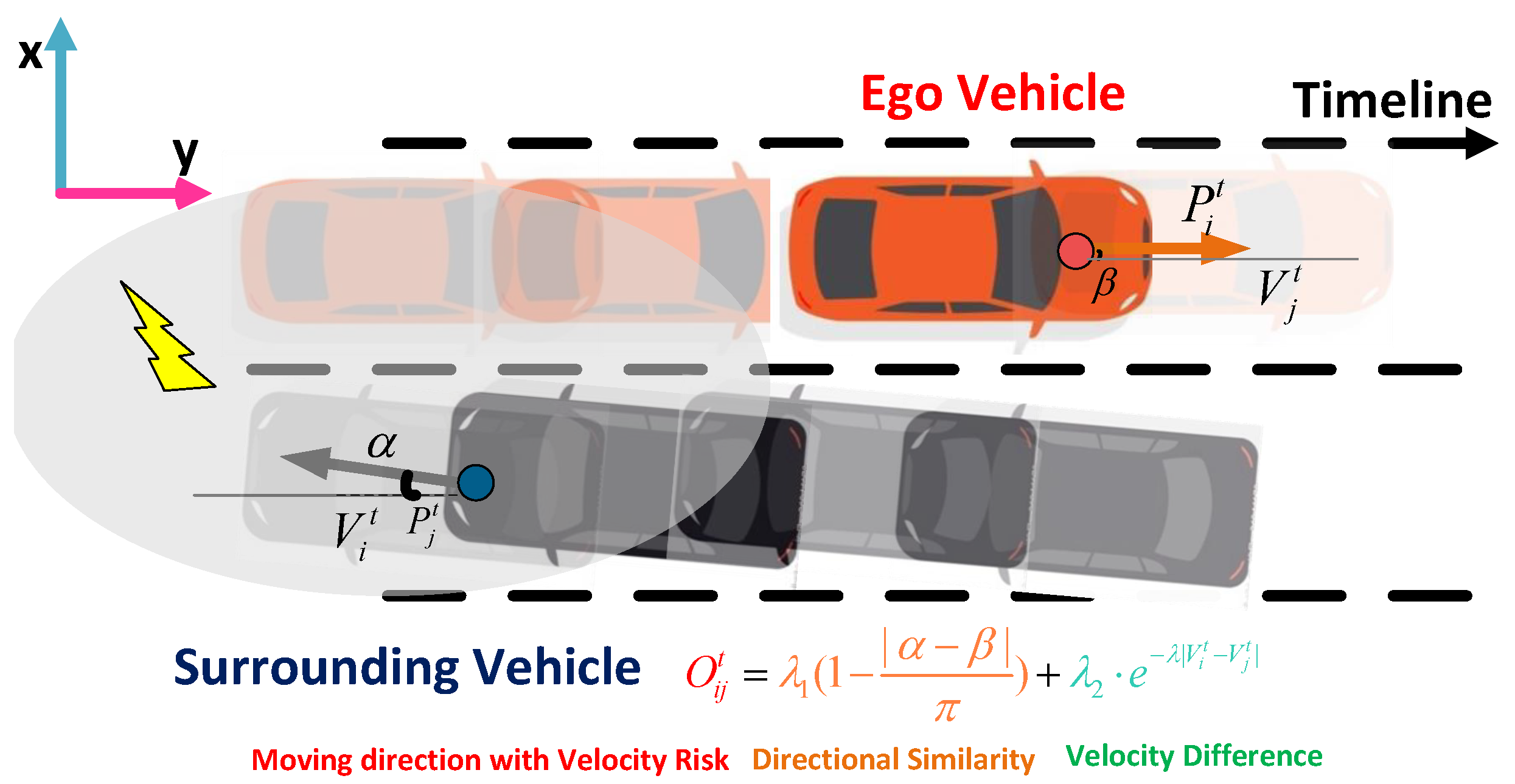
Moving Direction with Velocity Risk

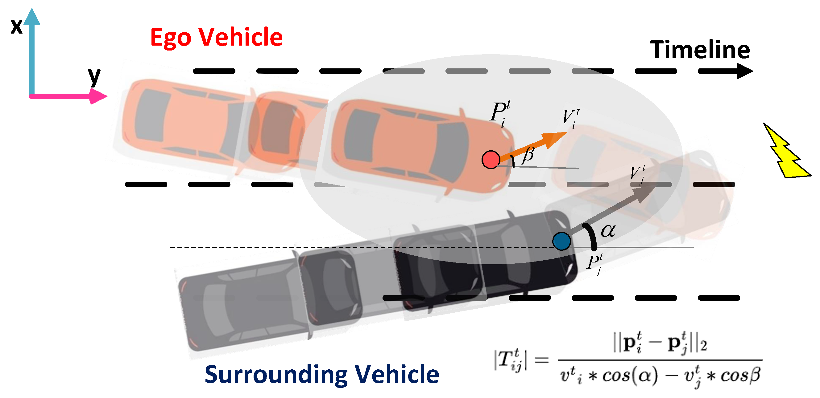
To accurately capture the dynamic interaction between agents, the velocity risk $O_{ij}^t$ is formulated as follows:

$$O_{ij}^t={\lambda }_1\left(1-{\displaystyle \frac{|\alpha -\beta |}{\pi }}\right)+{\lambda }_2·e^{-\lambda |V_i^t-V_j^t|}.$$

(4)

Directional Similarity: The term $1-{\displaystyle \frac{|\alpha -\beta |}{\pi }}$ represents the angular relationship between the movement directions of agents i and j. Here, $\alpha$ and $\beta$ denote the angles of the velocities of agents i and j, respectively. It provides a smoother measure of directional influence, where a value of 1 indicates that the agents are moving in the same direction, and a value of 0 indicates they are moving in exactly opposite directions. Unlike the cosine function, this term ensures that even when the agents move in opposite directions, there is still some influence on the trajectory prediction.

Velocity Difference: The second component $e^{-\lambda |V_i^t-V_j^t|}$ accounts for the difference in velocities between the two agents, where $V_i^t$ and $V_j^t$ represent the velocities of agents i and j at time t. It uses exponential decay to smoothly handle velocity differences. As the difference increases, the value decreases gradually, avoiding abrupt changes and ensuring a natural weight adjustment.

By combining these two components, $O_i{j}^t$ effectively captures both the directional influence and the velocity similarity of the agents. This formulation enhances the understanding of dynamic interactions in multi-agent systems, allowing for more accurate modeling of their behaviors and relationships, even when agents move in opposite directions.

Time to Collision

In Figure 5, the time that remains until a collision between two vehicles would occur if they keep their current speeds has been widely utilized to measure the driving risk for vehicle collision warning or avoidance.

$$|T_{ij}^t|={\displaystyle \frac{\left|\right|{\mathbf{p}}_i^t-{\mathbf{p}}_j^t{\left|\right|}_2}{v_i^t·cos\alpha -v_j^t·cos\beta }}$$

(5)

where $p_i^t$ and $p_j^t$ denote the locations of agent i and agent j at time t, respectively. $\alpha$ and $\beta$ are the handing angles of agent i and j.

Edge Index via Graph Optimization and Clustering

In Figure 6, we used the Gaussian kernel to compute edge distance $\left(e^{-\frac{\left|\right|{\mathbf{p}}_t^i-{\mathbf{p}}_t^j{\left|\right|}^2}{2\sigma }}\right)$, where $p_t^i$ and $p_t^j$ are agent i and j position. The kernel distance between all trajectory samples is used to build the affinity matrix W. Spectral clustering is employed to divide the nodes into different groups. Based on the clustering results, the graph is segmented into different subgraphs using minimum cut. We used the minimum cut algorithm on the graph represented by the adjacency matrix W, which is derived from the Laplacian matrix shown below:

$$L=D-W,$$

(6)

where D is the degree matrix of W. The normalized Laplacian matrix $D^{-\frac{1}{2}}L{D}^{-\frac{1}{2}}$ can also be used to facilitate graph partitioning. By the clustering process, we can obtain $C_i^t$ and $C_j^t$ to represent the cluster index of agent i and agent j, respectively, corresponding to the moving patterns clustered by the trajectories.

In conclusion, spectral clustering not only provides a powerful tool for dividing nodes into different groups but also employs minimum cut optimization to enhance the clustering results. Our method, by leveraging the Gaussian kernel for computing points distances, building affinity matrices, and optimizing with the minimum cut of the Laplacian matrix, enables a more accurate representation of the relationships between agents. This comprehensive method holds great promise for applications in trajectory prediction and analysis of complex systems involving multiple agents.

3.3.2. Risk-Aware Edge Graph Attention

The neighborhood nodes are enriched with risk-aware features through message passing and an attention mechanism, enabling the central agent to capture risk-aware attributes. The central agent’s embedding is then transformed into the query vector, while the embeddings of neighboring agents, enhanced with risk-aware attributes, are used to compute the key and value vectors:

$${\mathbf{q}}_i^t={\mathbf{W}}^{Q^{\mathrm{space}}}{\mathbf{z}}_i^t,{\mathbf{k}}_{ij}^t={\mathbf{W}}^{K^{\mathrm{space}}}{\mathbf{m}}_{ij}^t,{\mathbf{v}}_{ij}^t={\mathbf{W}}^{V^{\mathrm{space}}}{\mathbf{m}}_{ij}^t$$

(7)

where ${\mathbf{W}}^{Q^{\mathrm{space}}},{\mathbf{W}}^{K^{\mathrm{space}}},{\mathbf{W}}^{V^{\mathrm{space}}}\in {\mathbb{R}}^{d_k\times d_h}$ are learnable matrices for linear projection, and $d_k$ is the dimension of the transformed vectors.

The enhanced risk-aware edge (3) operates on the resulting query, key, and value vectors, which are taken as inputs to the scaled dot-product attention block:

$${\alpha }_i^t=\mathrm{softmax}\left({\displaystyle \frac{{\mathbf{q}}_i^{t\top }}{\sqrt{d_k}}}·\left[{\left\{{\mathbf{k}}_{ij}^t\right\}}_{j\in {\mathcal{N}}_i}\right]\right)$$

(8)

$${\mathbf{o}}_i^t=\sum _{j\in {\mathcal{N}}_i}{\alpha }_{ij}^t{\mathbf{v}}_{ij}^t,$$

(9)

$${\mathbf{g}}_i^t=\mathrm{sigmoid}\left({\mathbf{W}}^{\mathrm{gate}}\left[{\mathbf{z}}_i^t,{\mathbf{o}}_i^t\right]\right),$$

(10)

$${\widehat{\mathbf{z}}}_i^t={\mathbf{g}}_i^t\odot {\mathbf{W}}^{\mathrm{self}}{\mathbf{z}}_i^t+\left(1-{\mathbf{g}}_i^t\right)\odot {\mathbf{o}}_i^t,$$

(11)

where ${\mathcal{N}}_i$ is the set of agent $i’s$ neighbors, $W^{gate}$ and $W^{self}$ are learnable matrices, and ⊙ denotes elementwise product.

Compared to the standard scaled dot-product attention, our variant uses a gating function to fuse the environmental features $m_i^t$ with the central agent’s features, enabling the block to have more control over the feature update. The outputs of the multi-head attention block are passed through an MLP block to obtain the spatial embedding of agent i at time step t. In addition, we applied layer normalization before each block and residual connections after each block. In practice, this module can be implemented using efficient scatter and gather operations to parallelize the learning across all local regions and all time steps.

3.3.3. Low-Rank Temporal Transformer

By introducing a temporal encoder layer, we can effectively capture temporal feature representations following the spatial multi-agent encoding, thereby enhancing the model’s performance in time series prediction tasks. Inspired by Linformer [26], we designed a low-rank temporal transformer layer to further optimize efficiency and scalability.

We first add learnable positional embeddings to all tokens and stack the tokens into a matrix ${\mathbf{C}}_i\in {\mathbb{R}}^{(T+1)\times N\times D}$, which is then fed into the temporal attention block: The temporal attention block includes a mask and a linear layer to extend address the input. The mask M is used for certain positions to contribute to the attention score:

$${\tilde{C}}_i={\mathbf{C}}_i+M$$

(12)

$$M_{ij}=\left\{\begin{array}{cc}-\infty \hfill & \mathrm{if}\mathrm{position}i\mathrm{is}\mathrm{masked}\mathrm{for}\mathrm{position}j\hfill \\ 0\hfill & \mathrm{otherwise}\hfill \end{array}\right.$$

(13)

In the context of low-rank approximation, the singular value decomposition (SVD) allows us to decompose a matrix into its fundamental components. The singular values represent the importance of each mode in the original matrix. According to the Eckart–Young theorem [32], the best rank-k approximation of a matrix, in terms of minimizing the reconstruction error, is obtained by retaining only the top-k largest singular values and their corresponding singular vectors. This means that by preserving the top-k singular values, we can capture the most significant information in the data while reducing the dimensionality, thereby achieving an optimal trade-off between computational efficiency and information retention.

To reduce the computational complexity of the attention mechanism, we applied a low-rank approximation to the query (Q), key (K), and value (V) matrices. This method enables efficient processing by approximating these matrices with lower-rank representations.

Singular Value Decomposition

We perform SVD on the query matrix Q to obtain its low-rank approximation. Let the SVD of Q be defined as follows:

$$Q=U\Sigma V^{\top },$$

(14)

where $U\in {\mathbb{R}}^{d\times d}$ and $V^{\top }\in {\mathbb{R}}^{d\times d}$ are orthogonal matrices, and $\Sigma \in {\mathbb{R}}^{d\times d}$ is a diagonal matrix of singular values. We select the top k singular values to obtain the low-rank approximation:

$$Q_{\mathrm{low}\mathrm{rank}}=U_{[:,1:k]}{\Sigma }_{[1:k,1:k]}{V}_{[1:k,:]}^{\top },$$

(15)

where k is the chosen rank of the approximation. This reduces the dimensions of Q while retaining the most important information.

Low-Rank Approximation for K and V

Similarly, we apply the low-rank approximation to the key matrix K and value matrix V:

$$K_{\mathrm{low}\mathrm{rank}}=U_{[:,1:k]}{\Sigma }_{[1:k,1:k]}{V}_{[1:k,:]}^{\top },$$

(16)

$$V_{\mathrm{low}\mathrm{rank}}=U_{[:,1:k]}{\Sigma }_{[1:k,1:k]}{V}_{[1:k,:]}^{\top }.$$

(17)

This ensures that both K and V are approximated in the same way as Q, reducing their dimensions to rank k.

Attention Computation with Low-Rank Q, K, V

The low-rank matrices are then used to compute the scaled dot-product attention:

$$\mathrm{Attention}(Q,K,V)=\mathrm{softmax}\left({\displaystyle \frac{Q_{\mathrm{low}\mathrm{rank}}{K}_{\mathrm{low}\mathrm{rank}}^{\top }}{\sqrt{d_k}}}\right)V_{\mathrm{low}\mathrm{rank}},$$

(18)

where $d_k$ is the dimension of the key vectors. The result is a low-rank attention matrix that significantly reduces the computational complexity while preserving the core structure of the attention mechanism.

By utilizing low-rank approximations in this way, the overall computational complexity of the attention mechanism is reduced from $O\left(N^{2}D\right)$ to $O(N^{2}k+NDk)$. In our case, k is moderately smaller than D, reducing from 128 to 96 dimensions, which provides some computational savings while still retaining a substantial amount of the original information.

3.4. Fusion Lane and Global Interaction Encoder

After embedding the risk-aware agent local spatial and temporal information, the spatial layout of the local map is key to forecasting an agent’s future trajectory. To integrate map data effectively, we first align the relative positions of lane segments with the agent’s reference frame at time step T by rotating the lane vectors.

These transformed lane vectors, along with their semantic attributes, are passed through an MLP to generate lane-embedded features of Lane–agents fusion:

$$L_{i\phi }={\varphi }_{\mathrm{lane}}\left(\left[\begin{array}{c}{\mathbf{R}}_i^{\top }\left({\mathbf{p}}_{\phi }^1-{\mathbf{p}}_{\phi }^0\right),{\mathbf{R}}_i^{\top }\left({\mathbf{p}}_{\phi }^0-{\mathbf{p}}_i^T\right),a_{\phi }\end{array}\right]\right),$$

(19)

where ${\varphi }_{\mathrm{lane}}(·)$ refers to the MLP that encodes the lane segments, ${\mathbf{R}}_i$ is the rotation matrix for agent i to align and ${\mathbf{p}}_{\phi }^0$, and ${\mathbf{p}}_{\phi }^1$ represents the lane segment start and end points of lane segment $\phi$. Lane attribute is $a_{\phi }$. The attention between the central agent and the lane is then computed using Equations (7)–(11), with the agent’s state serving as the query and the lane information as keys and values.

For modeling broader interactions among agents and fusion map agents, we introduce global attention based on relative positions and orientations. The interaction between agents i and j is captured by encoding their positional and angular differences through an MLP:

$$e_{ij}^{\mathrm{global}}={\varphi }_{\mathrm{glo}}\left(\left[{\mathbf{R}}_i^T\left({\mathbf{p}}_j^T-{\mathbf{p}}_i^T\right),cos(\Delta {\alpha }_{ij}),sin(\Delta {\alpha }_{ij})\right]\right).$$

(20)

where $\Delta {\alpha }_{ij}$ denotes the angular difference, while the spatial vectors encode positional relationships. These global interaction embeddings are further processed using attention mechanisms, where each agent’s embedding serves as the query and the pairwise global edge information which, combined with neighboring agent features, are used as keys and values like local encoder. This fusion map and global interaction layer integrates local agent–lane relations with global agent-to-agent relations enhanced with risk-aware interactions, allowing for robust trajectory prediction.

3.5. Continuous Parameterized Trajectory Decoder

After symmetric global feature fusion, the updated actor tokens are collected and passed through a multi-modal motion decoder to generate predictions for all agents. This allows the decoder to forecast K possible future trajectories for each agent. For each trajectory mode, we use an MLP with two heads: a regression head for predicting the trajectory locations and a classification head followed by a softmax function to provide the corresponding probability scores. The advantage of this approach lies in its ability to predict multiple potential future trajectories, capturing the inherent uncertainty and variability in agent behavior, which is crucial for accurate and robust forecasting in complex autonomous driving environments.

For trajectory regression, instead of directly predicting the location, we generate control points for a continuous parameterized trajectory curve using the extracted features from the encoder. These control points are combined with basis functions, which are influenced by a dynamically adjusted knot vector based on velocity and curvature. The benefit of using control points with a dynamic knot vector is that it allows the model to flexibly adapt to changing speeds and curvatures, making it highly suitable for autonomous driving applications.

As shown in Figure 7, a B-spline (Basis Spline) is a piecewise-defined polynomial function used to represent curves for trajectory prediction because of their ability to provide smooth and continuous curves while maintaining control over local segments.

3.5.1. B-Spline Curve

B-Spline Representation

Given control points $P_i=(x_i,y_i)$ and the corresponding basis functions $N_{i,p}\left(t\right)$, the B-spline curve is computed as follows:

$$C\left(t\right)=\sum _{i=0}^n{N}_{i,d}\left(t\right)P_i,t\in [t_{k,i},t_{k,i}+T_i]$$

(21)

where $P_i$ defines the i-th control points, and $N_{i,d}\left(t\right)$ is the B-spline basis function of degree $d=5$, defined over a knot vector t. For a historical time range $T_i$, agent i at time k means $t_{k,i}$.

B-Spline Basis Function

B-spline basis function defines how each control point influences the shape of the curve. It is recursively defined as follows:

Initial basis function (0th degree)

$$N_{i,0}\left(t\right)=\left\{\begin{array}{cc}1\hfill & \mathrm{if}{t}_i\le t<t_{i+1}\hfill \\ 0\hfill & \mathrm{otherwise}\hfill \end{array}\right.$$

(22)

Recursive basis function (degree p)

$$N_{i,d}\left(t\right)={\displaystyle \frac{t-v_i}{v_{i+d}-v_i}}{N}_{i,d-1}\left(t\right)+{\displaystyle \frac{v_{i+d+1}-t}{v_{i+d+1}-v_{i+1}}}{N}_{i+1,d-1}\left(t\right),$$

(23)

where t is the parameter, $v_i$ is the i-th knot value in the knot vector, and d is the degree of the B-spline.

3.5.2. Knot Vector Adaptation

Knot Vector Adaption

In our approach, we initialize the knot vector as a uniform sequence, ensuring an even distribution of control points at the beginning of the trajectory generation. Specifically, the knot vector for a B-spline curve with n control points is defined as follows:

$$v_0=0,v_1={\displaystyle \frac{1}{n}},v_2={\displaystyle \frac{2}{n}},\dots ,v_n=1.$$

(24)

This uniform initialization is used for the first 5 frames to ensure a balanced and smooth trajectory prediction.

Starting from the 6th frame, we introduce an adaptive adjustment of the knot vector based on the vehicle’s velocity and curvature at each step. The new knot vector $v_j$ is updated based on the following formula:

$$v_j=\alpha e^{-\left(|C^{\prime }\left(v\right)\left|\right(1+\beta \left|\kappa \left(v\right)\right|)\right)}$$

(25)

Therein, we have the following:

• $v_j$ is the new knot vector value at the j-th position;
• $\alpha$ is a scaling factor that controls the adjustment magnitude;
• $C^{\prime }\left(v\right)$ is the velocity of the trajectory at point v;
• $\kappa \left(v\right)$ is the curvature of the trajectory at point v;
• $\beta$ is a weight parameter that controls the influence of curvature on the adjustment.

This exponential adjustment ensures that larger velocities or curvatures result in smaller changes to the knot vector, promoting smoother transitions in dynamically changing regions of the trajectory. Conversely, when both velocity and curvature are small, the knot vector is adjusted more significantly, allowing for finer control over the trajectory’s shape. This dynamic adaptation of the knot vector enables the trajectory to better reflect real-world motion characteristics, especially in scenarios involving sharp turns or rapid speed changes.

By updating the knot vector in this manner, we enhance the flexibility of the trajectory representation, ensuring that it adapts to both gradual and sudden changes in vehicle dynamics. The process is repeated for all subsequent frames from the 6th frame onward, continuously refining the trajectory prediction as more frames are generated.

Velocity Calculation The velocity of the B-spline curve can be calculated by differentiating the curve once. Given the B-spline curve $C\left(t\right)$, its velocity is computed as follows:

$$C^{\prime }\left(t\right)=\sum _{i=0}^n{N}_{i,d}^{\prime }\left(t\right)P_i$$

(26)

The Calculation of Curvature The calculation of curvature $\kappa \left(t\right)$ is used to describe the degree of bending of a curve, and it depends on both the first and second derivatives of the curve. The formula for curvature is as follows:

$$\kappa \left(t\right)={\displaystyle \frac{C^{\prime }\left(t\right)\times C^{\prime \prime }\left(t\right)}{|C^{\prime }{\left(t\right)|}^3}}$$

(27)

where $C^{\prime }\left(t\right)$ represents the first derivative of the curve corresponding to the velocity. $C^{\prime \prime }\left(t\right)$ represents the second derivative of the curve corresponding to the acceleration. ×denotes the cross product, and $|C^{\prime }\left(t\right)|$ represents the magnitude of the first derivative (velocity magnitude).

This formula is typically used in trajectory prediction tasks to calculate the curvature of B-spline curves, helping to assess the smoothness and degree of bending of predicted trajectories.

3.5.3. Predicted Trajectory Matrix

The trajectory matrix ${\mathbf{Y}}_{pos}$, which contains the 2D positions for T timestamps, can be computed by performing matrix multiplication between the B-spline basis matrix ${\mathbf{B}}_{\mathbf{u}}$ and the predicted 2D control points matrix $\mathbf{P}$:

$${\mathbf{Y}}_{pos}={\mathbf{B}}_{\mathbf{u}}\mathbf{P}$$

(28)

where ${\mathbf{Y}}_{pos}\in {\mathbb{R}}^{T\times 2}$ can be calculated by multiplying the adaptive basis matrix. ${\mathbf{B}}_{\mathbf{u}}\in {\mathbb{R}}^{T\times (n+1)}$ is the precomputed B-spline basis matrix, where $\mathbf{B}$ is the updated knot vector that adjusts according to velocity and curvature changes. This matrix represents the contribution of each control point to the final trajectory across T time steps.

The control points matrix $\mathbf{P}\in {\mathbb{R}}^{(n+1)\times 2}$ contains the predicted 2D control points for the trajectory, where each row represents the x and y coordinates of a control point.

The positional coordinates at each time step can be computed as follows:

$${\mathbf{Y}}_{\mathrm{pos}}=\left[\begin{array}{cccc}{\mathbf{N}}_{0,k}\left(u_{t_1}\right)& {\mathbf{N}}_{1,k}\left(u_{t_1}\right)& \cdots & {\mathbf{N}}_{n,k}\left(u_{t_1}\right)\\ {\mathbf{N}}_{0,k}\left(u_{t_2}\right)& {\mathbf{N}}_{1,k}\left(u_{t_2}\right)& \cdots & {\mathbf{N}}_{n,k}\left(u_{t_2}\right)\\ ⋮& ⋮& \ddots & ⋮\\ {\mathbf{N}}_{0,k}\left(u_T\right)& {\mathbf{N}}_{1,k}\left(u_T\right)& \cdots & {\mathbf{N}}_{n,k}\left(u_T\right)\end{array}\right]\left[\begin{array}{cc}{\mathbf{p}}_0^x& {\mathbf{p}}_0^y\\ {\mathbf{p}}_1^x& {\mathbf{p}}_1^y\\ ⋮& ⋮\\ {\mathbf{p}}_n^x& {\mathbf{p}}_n^y\end{array}\right]$$

(29)

where $N_{i,k}\left(u_{t_j}\right)$ is the B-spline basis function of degree k evaluated at the adaptive knot vector value $u_{t_j}$. The adaptive knot vector ${\mathbf{u}}_{t_j}$ is calculated based on the vehicle’s velocity and curvature at each step, ensuring that the knot values are dynamically adjusted to better fit the trajectory.

By multiplying the adaptive B-spline basis matrix ${\mathbf{B}}_{\mathbf{u}}$ with the control points matrix $\mathbf{P}$, we obtain the full set of predicted positions for the trajectory that account for dynamic changes in curvature and velocity. Our proposed method ensures that trajectory generation remains adaptive and responsive to real-time conditions, leading to smoother transitions and more accurate trajectory predictions, which are essential for autonomous vehicles.

4. Expertiments

4.1. Experiments Setup

4.1.1. Datasets

Our evaluation was conducted on the large-scale Argoverse motion forecasting dataset [33], which provides detailed agent trajectories along with high-definition map data to support autonomous vehicle perception tasks. It consists of over 323,000 real-world driving scenarios split into 205,942 training samples, 39,472 validation samples, and 78,143 test samples. Each scenario consists of 5-second sequences sampled at 10 Hz, with only the first 2 s available in the test set, where participants are tasked with predicting the subsequent 3-second future trajectories for agents.

4.1.2. Evaluation Metrics

Let the multi-mode prediction of the model be represented as below:

$$O={\left\{\left(p_1^k,p_2^k,\dots ,p_T^k\right)\right\}}_{k\in [1,K]},$$

(30)

where $p_t^k=(x_t^k,y_t^k)$ is the predicted position of the agent at time step t for the k-th mode. The ground truth trajectory of the agent is denoted as $O^{*}=(p_1^{*},p_2^{*},\dots ,p_T^{*})$. Our model was assessed using widely accepted metrics for motion prediction tasks, including minimum Average Displacement Error (minADE), minimum Final Displacement Error (minFDE), and Miss Rate (MR). These metrics enable the model to predict up to six potential trajectories for each agent. Specifically, minADE represents the average ${\ell }_2$ distance in meters between the predicted trajectory with the lowest error and the actual ground-truth trajectory across all time steps. In contrast, minFDE measures the prediction error at the final time step. The trajectory with the smallest endpoint error is considered the best prediction. Meanwhile, MR refers to the proportion of cases where the distance between the predicted and ground-truth endpoints exceeds 2.0 m.

Minimum Average Displacement Error (minADE)

This is the minimum value of the Euclidean distance between the predicted and ground truth trajectories, which is averaged over the prediction length T for K predicted modes. It measures how well the predictions match the ground truth on average under the Euclidean space. The detailed calculation is as follows:

$$minADE=\underset{k=1,\dots ,K}{min}{\displaystyle \frac{1}{T}}\sum _{t=1}^T{\parallel p_t^k-p_t^{*}\parallel }_2,$$

(31)

where $p_t^k$ is the predicted coordinate of the k-th mode at time step t, and $p_t^{*}$ is the ground truth coordinate at time t, with T being the total length of the trajectory.

Minimum Final Displacement Error (minFDE)

This metric is similar to minADE, but it only considers the error at the final time step T. It focuses on the accuracy of predicting the final goal point, which emphasizes the importance of capturing agents’ intentions. The detailed calculation is as follows:

$$minFDE=\underset{k=1,\dots ,K}{min}{\parallel p_T^k-p_T^{*}\parallel }_2,$$

(32)

Miss Rate (MR)

The MR represents the ratio of cases where the Euclidean distance between the predicted and ground truth final positions exceeds 2 m for all k predicted modes. Unlike Euclidean-based metrics like minADE and minFDE, it only requires one of the predicted modes to fall near the ground truth final point for it to be considered a “hit”. If none of the predicted modes are within 2 m, it counts as a “miss”. The detailed calculation is as follows:

$$MR=\left\{\begin{array}{cc}0,\hfill & \exists k\in \{1,\dots ,K\},\parallel p_T^k-p_T^{*}{\parallel }_2\le 2\hfill \\ 1,\hfill & \mathrm{Otherwise}\hfill \end{array}\right.,$$

(33)

Note that all three metrics are averaged over all target agents.

4.1.3. Implementation Details

We trained our model for 64 epochs on an RTX 3090 GPU using an Adam optimizer [34], with the batch size, initial learning rate, weight decay, and dropout rate set to 32, $3\times {10}^{-4}$, $1\times {10}^{-4}$, and 0.1, respectively. The learning rate was decayed using the cosine annealing scheduler. We used a 1-layer heterogeneous risk-aware local graph attention encoder, which focuses on modeling the spatial relationships between agents. Additionally, our model incorporated a 4-layer temporal transformer to efficiently capture temporal dynamics. Both modules utilized multi-head attention with eight heads, allowing the model to focus on different interaction aspects. Furthermore, we included a 3-layer global interaction layer with a 1-layer fusion map lane with a multi-agent interaction module, which were introduced to specifically capture interactions between agents and lane information finally to model broader context interactions between agents. In addition, the hyperparameter settings presented in this work are shown in

Table 1. All hyperparameters set in this study.

Hyperparameter	Source	Value
$\lambda$	Equation (4)	$0.1$
${\lambda }_1$	Equation (4)	$0.65$
${\lambda }_2$	Equation (4)	$0.35$
$d_k$	Equation (19)	96
degree (d)	Section 3.5	5
$\alpha$	Equation (24)	$0.5$
$\beta$	Equation (24)	$0.3$

.

4.2. Ablation Studies

4.2.1. Ablation Studies on Each Encoder Component

We assessed the impact of each module by removing them alternately and observing the effects on prediction performance. As shown in

Table 2. Ablation studies on the components of our framework.

HRG	TD	${\mathbf{FGI}}_{\mathit{l}}$	${\mathbf{FGI}}_{\mathit{g}}$	minADE	minFDE	MR
	✓	✓	✓	0.71	1.07	0.11
✓		✓	✓	1.10	1.48	0.22
✓	✓		✓	0.69	1.01	0.13
✓	✓	✓		0.68	1.00	0.10
✓	✓	✓	✓	0.650	0.900	0.085

, each module contributed to the overall improvement in different ways. First, without the risk-aware agent-to-agent interaction module, the model struggled to capture critical local interactions, leading to performance degradation. Second, the low-rank temporal learning module had the most notable influence on performance, as predicting the future movements of agents in dynamic traffic situations heavily depends on efficiently leveraging historical information. Third, we separated the lane-specific interaction ($FG{I}_l$) and global interaction ($FG{I}_g$) to evaluate their respective impacts. Lane information remains essential for trajectory prediction, as traffic agents typically follow lanes constrained by traffic rules, while global interactions are also crucial for capturing the cross-agent and map-level dependencies over time. Lastly, the continuous parameterized trajectory decoding module significantly boosted the performance, showcasing its effectiveness in generating continuous and smooth future trajectories. This confirms its advantage over conventional methods in producing high-quality predictions.

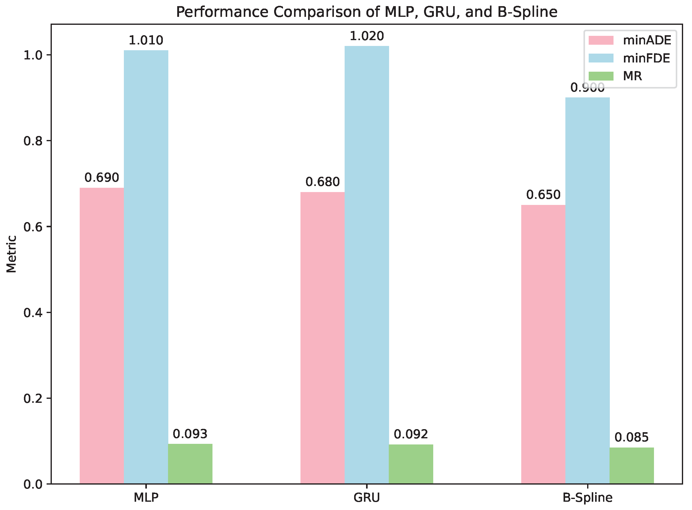
4.2.2. Ablation Study of Decoder Variants with Continuous Trajectory Decoder

As shown in Figure 8, in our experimental comparison of the three decoder variants MLP, GRU, and the proposed continuous parameterized decoder, the continuous parameterized model showed clear advantages across all evaluated metrics. The continuous parameterized decoder demonstrated superior performance in terms of prediction accuracy, particularly in the minADE, minFDE and MR, highlighting the benefits of using a continuous curve-based decoding approach for trajectory prediction. The continuous parameterized decoder achieved the lowest minADE at 0.65, demonstrating that the continuous parameterized decoder can better interpolate and extrapolate future positions. A lower MR indicates that the continuous parameterized decoder is better at generating realistic and feasible trajectories, which is crucial for safety-critical applications like autonomous driving.

Although the continuous parameterized decoder arrived at its results with a marginal increase in computational cost—both in terms of inference time (75 ms) and parameters (2839 K)—the improvements in prediction accuracy (minADE and minFDE) and the significant reduction in miss rate (MR) justify the slightly higher complexity.

4.3. Results

4.3.1. Comparison with State-of-the-Art

We briefly introduce the methods we compared on the Argoverse dataset.

TNT [7] uses discretized sparse anchors on roads for goal prediction, assigning probability values to these anchors. However, this approach has limitations, as it can only predict one goal per anchor and lacks the ability to capture fine-grained details, such as varying local information within the same lane segment.

DenseTNT [8] uses VectorNet as its encoder to model the scene as a homogeneous fully connected graph and employs an optimization-based technique to select the best goal from a dense set of candidates, which allows it to generate more diverse trajectory modes and achieve better MR performance than direct trajectory decoding.

LaneGCN [9] is a pioneering model in motion forecasting that constructs a lane graph from raw map data, extending graph convolutions with multiple adjacency matrices to preserve the complex map structure and capture long-range dependencies, enabling accurate and realistic multi-modal trajectory predictions by modeling intricate actor–map interactions.

LaneRCNN [10] Building upon LaneGCN, it advances the lane graph encoding approach by introducing a graph-centric model that learns localized lane graph representations (LaneRoI) for each actor, allowing for efficient actor-to-actor and actor-to-map interactions through message passing within a global lane graph, further enhancing trajectory prediction accuracy.

TPCN [24] leverages both spatial and temporal dimensions by applying point cloud learning techniques to represent agents as unordered point sets in space and introducing dynamic temporal learning to model agents’ motion over time.

R-Pred [35] is a two-stage trajectory prediction method that utilizes scene and interaction context through a tube-query scene attention mechanism and proposal-level interaction attention to refine trajectory proposals.

HVTD [36] proposes a hierarchical vector transformer diffusion model for vehicle trajectory prediction, combining local and global interactions with a diffusion convolutional encoder to effectively capture uncertainty.

HIVT [14] leverages hierarchical modeling of local and global interactions using Transformers for multi-agent motion prediction, incorporating translation- and rotation-invariant representations to efficiently predict trajectories with fewer parameters and faster.

We compared our method with the state-of-the-art models on the Argoverse validation set. Based on the results in

Table 3. Comparison with the state-of-the-art trajectory prediction on validation set of Argoverse.

Model	minADE	minFDE	MR
DESIRE [37]	0.92	1.77	0.18
DATF [38]	0.92	1.52
MultiPath [39]	0.80	1.68	0.14
LaneRCNN [10]	0.77	1.19	0.082
DenseTNT [8]	0.75	1.05	0.10
TNT [7]	0.73	1.29	0.093
TPCN [24]	0.73	1.15	0.11
LaneGCN [9]	0.71	1.08	0.10
R-Pred [35]	0.657	0.945	0.0869
HVTD [36]	0.68	1.02	0.10
HiVT-128 [14]	0.66	0.96	0.09
Ours	0.65	0.90	0.085

, our approach achieved the lowest average displacement error (ADE), outperforming HiVT-128 (0.66) by 0.01 and R-Pred (0.657) by a smaller margin of 0.007. Compared to DenseTNT (0.75) and TPCN (0.73), we recorded reductions of 0.10 and 0.08, respectively, demonstrating the robustness of our risk-aware interaction modeling. Our final displacement error (FDE) also performed exceptionally well, surpassing R-Pred (0.945) by 0.045 and showing a substantial reduction compared to DenseTNT (1.05), with a difference of 0.15. This significant improvement in the FDE can be attributed to our continuous parameterized trajectory decoding, which smooths and adapts trajectories effectively. In terms of the miss rate (MR), our approach achieved the best performance, outperforming LaneRCNN (0.082) by a slight margin of 0.003 and significantly beating DenseTNT (0.10) and TPCN (0.11), by 0.015 and 0.025, respectively. The superior MR performance demonstrates the strength of our risk-aware agent-to-agent interaction module in preventing missed predictions. In summary, our model’s minADE and minFDE improvements are largely driven by the effective combination of our risk-aware interaction modeling and continuous parameterized trajectory decoder. The significantly lower MR highlights the added value of our approach, especially in challenging prediction tasks, validating its superior performance over competing methods.

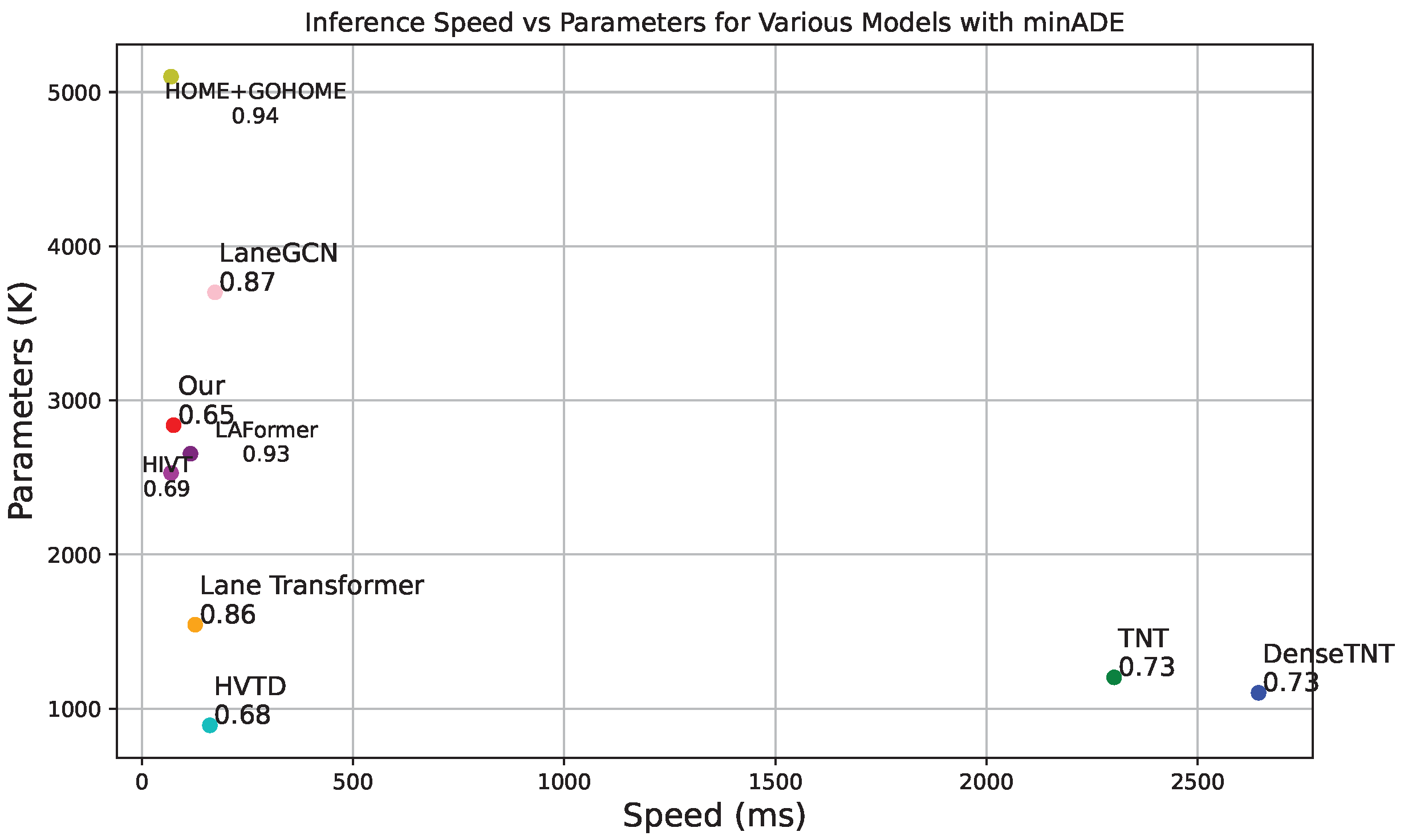
4.3.2. Inference Speed

We compared the inference speed of models on the Argoverse validation set as shown in Figure 9, where we can see that our model achieved an inference speed of 75 ms, positioning it in the mid-range when compared to other models. It outperformed computationally heavy models such as DenseTNT (2644 ms) and TNT [7] (2302 ms), which have significantly slower inference times. In contrast, models like HOME+GOHOME [12] (32 ms) and HIVT [14] (69 ms) exhibited faster inference times but with higher or comparable minADE values, indicating that our model strikes a good balance between speed and prediction accuracy. In terms of parameters, our model has 2839 K parameters, which is moderate compared to models like LaneGCN [9] (3701 K) and HOME+GOHOME [12] (5100 K). While our model is not the lightest, it achieved superior prediction accuracy with a minADE of 0.65. The parameter size is well within a practical range, offering an efficient balance between model complexity and performance. Our model stands out for its excellent prediction performance with a minADE of 0.65, which was the best among all compared models. Other models, such as TNT and DenseTNT [8], achieved minADEs of 0.73 and 0.75, respectively, but at the cost of significantly higher inference times. This showcases the strength of our model in making highly accurate predictions while maintaining reasonable speed and parameter sizes. The graph demonstrates our model as an optimal choice for scenarios requiring accurate and efficient trajectory prediction, making it highly suitable for real-time applications in autonomous systems.

4.3.3. Visualization

Intersection Successful Case

In Figure 10a, intersection successful case (a) (1) demonstrates a successful trajectory prediction using the heterogeneous multi-agent risk-aware graph approach. The predicted trajectory (in red) accurately follows the intended path, showcasing the method’s effectiveness in handling complex intersections with multiple agents. In Figure 10a(2), the prediction of six possible trajectories is shown, with the predicted trajectories (in red) corresponding well to the ground truth (in blue). It demonstrates the model’s ability to capture multiple future possibilities in highly dynamic intersection environments. In Figure 10a(3), the target agent accurately predicts that the neighboring agent in front will turn left in the future. This shows the model’s awareness of interactions between agents and its capacity to predict accurate trajectories based on future maneuvers. The success of this intersection case is due to the effectiveness of our heterogeneous risk-aware graph encoder in predicting accurate trajectories in complex intersection scenarios.

Continuous Parameterized Trajectory Prediction Performance Analysis

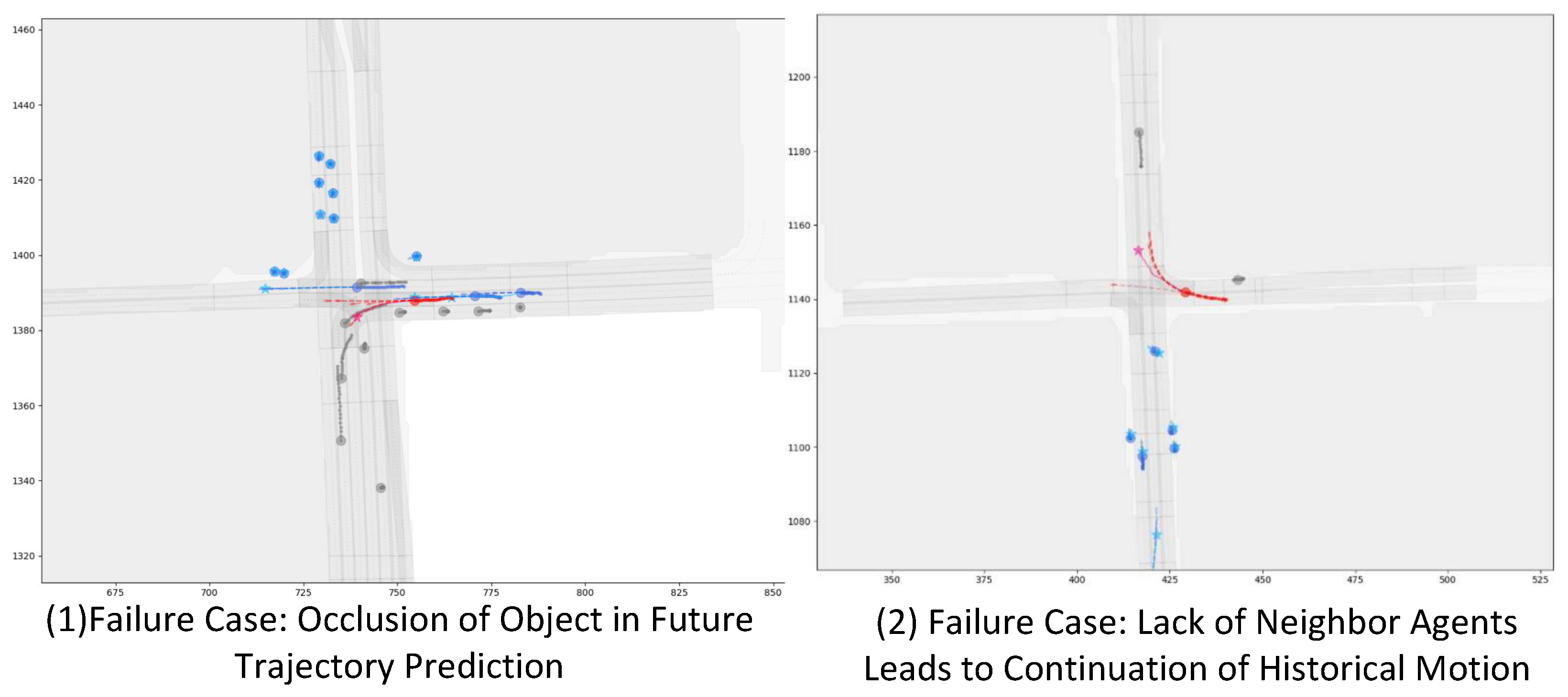
In Figure 10b, continuous parameterized trajectory prediction performance analysis (1) illustrates how the continuous parameterized trajectory decoder performed in a complex intersection scenario. The predicted trajectory (in red) is both smooth and accurately follows the intended path, highlighting the decoder’s ability to handle intricate road layouts. In Figure 10b(2), the continuous parameterized trajectory decoder effectively managed a situation where the predicted trajectory involved self-intersection within the intersection. In Figure 10b(3), under more straightforward cases, such as a direct path through an intersection, the continuous parameterized trajectory decoder handled the scenario with ease, producing a smooth and accurate trajectory without unnecessary complexity. The smoothness and continuity properties of the continuous parameterized trajectory decoder allow it to handle both complex intersections and simpler scenarios with great accuracy, as seen in this analysis.

Failure Case

In Figure 11, failure case (1) occurred due to an occlusion in the predicted trajectory area, leading to an incorrect prediction. The occluded object interfered with the accuracy of future trajectory predictions, causing deviations from the expected path. In failure case (2), the predicted trajectory continued to follow its historical motion pattern due to the absence of neighboring agents, leading to an inaccurate future prediction, as no interactions occurre to influence the trajectory. These failure cases highlight the current limitations of the model, especially in handling occlusions and scenarios without significant agent interactions. Future work should focus on improving the model’s ability to adapt to dynamic environments and handle unseen obstacles.

5. Conclusions

This work addresses the challenges of trajectory prediction for heterogeneous multi-agent interactions in autonomous driving scenarios. Traditional methods often struggle to capture fine-grained interactions between diverse agents, particularly overlooking occlusion risks at intersections and sudden motion stops. To bridge this gap, we propose HRGC, a novel framework that incorporates a heterogeneous multi-agent risk-aware graph encoder, a low-rank temporal transformer, a lane fusion and global interaction encoder, and a continuous parameterized trajectory decoder. The model explicitly integrates risk assessment into multi-agent heterogeneous graph interactions, enhancing both robustness and prediction accuracy. Key innovations include a risk-aware graph encoder that effectively captures potential collision information and a continuous parameterized trajectory decoder that dynamically adjusts for speed and curvature changes. Experimental results demonstrate that HRGC achieves superior performance in complex intersection scenarios, significantly improving trajectory prediction accuracy compared to existing approaches.

6. Limitations and Future Work

Despite its promising results, HRGC still faces challenges in certain scenarios. One key limitation is the handling of occluded objects, where the absence of visible neighboring agents can lead to suboptimal predictions. Another limitation lies in low-interaction environments, where fewer agents reduce the model’s ability to make robust predictions. Future work will address these limitations by exploring more effective occlusion-handling strategies and improving the model’s ability to make accurate predictions even in sparse environments. We plan to incorporate collaborative perception, thereby enhancing prediction performance under challenging conditions.

References

1. Sun, S.; Shi, C.; Wang, C.; Zhou, Q.; Sun, R.; Xiao, B.; Ding, Y.; Xi, G. Intra-Frame Graph Structure and Inter-Frame Bipartite Graph Matching with ReID-Based Occlusion Resilience for Point Cloud Multi-Object Tracking. Electronics 2024, 13, 2968. [Google Scholar] [CrossRef]
2. Sun, S.; Shi, C.; Wang, C.; Liu, X. A Novel Adaptive Graph Transformer For Point Cloud Object Detection. In Proceedings of the 2023 7th International Conference on Communication and Information Systems (ICCIS), Chongqing, China, 20–22 October 2023; pp. 151–155. [Google Scholar]
3. Sun, S.; Wang, C.; Liu, X.; Shi, C.; Ding, Y.; Xi, G. Spatio-Temporal Bi-directional Cross-frame Memory for Distractor Filtering Point Cloud Single Object Tracking. arXiv 2024, arXiv:2403.15831. [Google Scholar]
4. Salzmann, T.; Ivanovic, B.; Chakravarty, P.; Pavone, M. Trajectron++: Dynamically-feasible trajectory forecasting with heterogeneous data. In Proceedings of the Computer Vision—ECCV 2020: 16th European Conference, Glasgow, UK, 23–28 August 2020; Proceedings, Part XVIII 16. Springer: Cham, Switzerland, 2020; pp. 683–700. [Google Scholar]
5. Mo, X.; Huang, Z.; Xing, Y.; Lv, C. Multi-agent trajectory prediction with heterogeneous edge-enhanced graph attention network. IEEE Trans. Intell. Transp. Syst. 2022, 23, 9554–9567. [Google Scholar] [CrossRef]
6. Gao, J.; Sun, C.; Zhao, H.; Shen, Y.; Anguelov, D.; Li, C.; Schmid, C. Vectornet: Encoding hd maps and agent dynamics from vectorized representation. In Proceedings of the IEEE/CVF Conference on Computer Vision and Pattern Recognition, Seattle, WA, USA, 13–19 June 2020; pp. 11525–11533. [Google Scholar]
7. Zhao, H.; Gao, J.; Lan, T.; Sun, C.; Sapp, B.; Varadarajan, B.; Shen, Y.; Shen, Y.; Chai, Y.; Schmid, C.; et al. Tnt: Target-driven trajectory prediction. In Proceedings of the Conference on Robot Learning, Cambridge, MA, USA, 8–11 November 2021; pp. 895–904. [Google Scholar]
8. Gu, J.; Sun, C.; Zhao, H. Densetnt: End-to-end trajectory prediction from dense goal sets. In Proceedings of the the IEEE/CVF International Conference on Computer Vision, Montreal, QC, Canada, 10–17 October 2021; pp. 15303–15312. [Google Scholar]
9. Liang, M.; Yang, B.; Hu, R.; Chen, Y.; Liao, R.; Feng, S.; Urtasun, R. Learning lane graph representations for motion forecasting. In Proceedings of the Computer Vision—ECCV 2020: 16th European Conference, Glasgow, UK, 23–28 August 2020; Proceedings, Part II 16. Springer: Cham, Switzerland, 2020; pp. 541–556. [Google Scholar]
10. Zeng, W.; Liang, M.; Liao, R.; Urtasun, R. Lanercnn: Distributed representations for graph-centric motion forecasting. In Proceedings of the 2021 IEEE/RSJ International Conference on Intelligent Robots and Systems (IROS), Prague, Czech Republic, 27 September–1 October 2021; pp. 532–539. [Google Scholar]
11. Gilles, T.; Sabatini, S.; Tsishkou, D.; Stanciulescu, B.; Moutarde, F. Home: Heatmap output for future motion estimation. In Proceedings of the 2021 IEEE International Intelligent Transportation Systems Conference (ITSC), Indianapolis, IN, USA, 19–22 September 2021; pp. 500–507. [Google Scholar]
12. Gilles, T.; Sabatini, S.; Tsishkou, D.; Stanciulescu, B.; Moutarde, F. Gohome: Graph-oriented heatmap output for future motion estimation. In Proceedings of the 2022 International Conference on Robotics and Automation (ICRA), Philadelphia, PA, USA, 23–27 May 2022; pp. 9107–9114. [Google Scholar]
13. Jia, X.; Wu, P.; Chen, L.; Liu, Y.; Li, H.; Yan, J. Hdgt: Heterogeneous driving graph transformer for multi-agent trajectory prediction via scene encoding. IEEE Trans. Pattern Anal. Mach. Intell. 2023, 45, 13860–13875. [Google Scholar] [CrossRef] [PubMed]
14. Zhou, Z.; Ye, L.; Wang, J.; Wu, K.; Lu, K. Hivt: Hierarchical vector transformer for multi-agent motion prediction. In Proceedings of the IEEE/CVF Conference on Computer Vision and Pattern Recognition, New Orleans, LA, USA, 18–24 June 2022; pp. 8823–8833. [Google Scholar]
15. Fang, J.; Zhu, C.; Zhang, P.; Yu, H.; Xue, J. Heterogeneous trajectory forecasting via risk and scene graph learning. IEEE Trans. Intell. Transp. Syst. 2023, 24, 12078–12091. [Google Scholar] [CrossRef]
16. Liu, X.; Wang, Y.; Jiang, K.; Zhou, Z.; Nam, K.; Yin, C. Interactive trajectory prediction using a driving risk map-integrated deep learning method for surrounding vehicles on highways. IEEE Trans. Intell. Transp. Syst. 2022, 23, 19076–19087. [Google Scholar] [CrossRef]
17. Varadarajan, B.; Hefny, A.; Srivastava, A.; Refaat, K.S.; Nayakanti, N.; Cornman, A.; Chen, K.; Douillard, B.; Lam, C.P.; Anguelov, D.; et al. Multipath++: Efficient information fusion and trajectory aggregation for behavior prediction. In Proceedings of the 2022 International Conference on Robotics and Automation (ICRA), Philadelphia, PA, USA, 23–27 May 2022; pp. 7814–7821. [Google Scholar]
18. Shi, S.; Jiang, L.; Dai, D.; Schiele, B. Motion transformer with global intention localization and local movement refinement. Adv. Neural Inf. Process. Syst. 2022, 35, 6531–6543. [Google Scholar]
19. Zhang, L.; Li, P.; Liu, S.; Shen, S. SIMPL: A Simple and Efficient Multi-agent Motion Prediction Baseline for Autonomous Driving. IEEE Robot. Autom. Lett. 2024, 9, 3767–3774. [Google Scholar] [CrossRef]
20. Kipf, T.N.; Welling, M. Semi-supervised classification with graph convolutional networks. arXiv 2016, arXiv:1609.02907. [Google Scholar]
21. Veličković, P.; Cucurull, G.; Casanova, A.; Romero, A.; Lio, P.; Bengio, Y. Graph attention networks. arXiv 2017, arXiv:1710.10903. [Google Scholar]
22. Wang, X.; Ji, H.; Shi, C.; Wang, B.; Ye, Y.; Cui, P.; Yu, P.S. Heterogeneous graph attention network. In Proceedings of the World Wide Web Conference, San Francisco, CA, USA, 13–17 May 2019; pp. 2022–2032. [Google Scholar]
23. Hong, H.; Guo, H.; Lin, Y.; Yang, X.; Li, Z.; Ye, J. An attention-based graph neural network for heterogeneous structural learning. AAAI Conf. Artif. Intell. 2020, 34, 4132–4139. [Google Scholar] [CrossRef]
24. Ye, M.; Cao, T.; Chen, Q. Tpcn: Temporal point cloud networks for motion forecasting. In Proceedings of the IEEE/CVF Conference on Computer Vision and Pattern Recognition, Nashville, TN, USA, 20–25 June 2021; pp. 11318–11327. [Google Scholar]
25. Zhang, Y.; Qian, D.; Li, D.; Pan, Y.; Chen, Y.; Liang, Z.; Zhang, Z.; Zhang, S.; Li, H.; Fu, M.; et al. Graphad: Interaction scene graph for end-to-end autonomous driving. arXiv 2024, arXiv:2403.19098. [Google Scholar]
26. Wang, S.; Li, B.Z.; Khabsa, M.; Fang, H.; Ma, H. Linformer: Self-attention with linear complexity. arXiv 2020, arXiv:2006.04768. [Google Scholar]
27. Li, Y.; Li, K.; Zheng, Y.; Morys, B.; Pan, S.; Wang, J. Threat assessment techniques in intelligent vehicles: A comparative survey. IEEE Intell. Transp. Syst. Mag. 2020, 13, 71–91. [Google Scholar] [CrossRef]
28. Lee, D.N. A theory of visual control of braking based on information about time-to-collision. Perception 1976, 5, 437–459. [Google Scholar] [CrossRef] [PubMed]
29. Minderhoud, M.M.; Bovy, P.H. Extended time-to-collision measures for road traffic safety assessment. Accid. Anal. Prev. 2001, 33, 89–97. [Google Scholar] [CrossRef] [PubMed]
30. Wang, X.; Alonso-Mora, J.; Wang, M. Probabilistic risk metric for highway driving leveraging multi-modal trajectory predictions. IEEE Trans. Intell. Transp. Syst. 2022, 23, 19399–19412. [Google Scholar] [CrossRef]
31. Tang, B.; Zhong, Y.; Neumann, U.; Wang, G.; Chen, S.; Zhang, Y. Collaborative uncertainty in multi-agent trajectory forecasting. Adv. Neural Inf. Process. Syst. 2021, 34, 6328–6340. [Google Scholar]
32. Eckart, C.; Young, G. The approximation of one matrix by another of lower rank. Psychometrika 1936, 1, 211–218. [Google Scholar] [CrossRef]
33. Chang, M.F.; Lambert, J.; Sangkloy, P.; Singh, J.; Bak, S.; Hartnett, A.; Wang, D.; Carr, P.; Lucey, S.; Ramanan, D.; et al. Argoverse: 3d tracking and forecasting with rich maps. In Proceedings of the IEEE/CVF Conference on Computer Vision and Pattern Recognition, Long Beach, CA, USA, 15–20 June 2019; pp. 8748–8757. [Google Scholar]
34. Loshchilov, I. Decoupled weight decay regularization. arXiv 2017, arXiv:1711.05101. [Google Scholar]
35. Choi, S.; Kim, J.; Yun, J.; Choi, J.W. R-pred: Two-stage motion prediction via tube-query attention-based trajectory refinement. In Proceedings of the IEEE/CVF International Conference on Computer Vision, Paris, France, 1–6 October 2023; pp. 8525–8535. [Google Scholar]
36. Tang, Y.; He, H.; Wang, Y. Hierarchical vector transformer vehicle trajectories prediction with diffusion convolutional neural networks. Neurocomputing 2024, 580, 127526. [Google Scholar] [CrossRef]
37. Lee, N.; Choi, W.; Vernaza, P.; Choy, C.B.; Torr, P.H.; Chandraker, M. Desire: Distant future prediction in dynamic scenes with interacting agents. In Proceedings of the IEEE Conference on Computer Vision and Pattern Recognition, Honolulu, HI, USA, 21–26 July 2017; pp. 336–345. [Google Scholar]
38. Park, S.H.; Lee, G.; Seo, J.; Bhat, M.; Kang, M.; Francis, J.; Jadhav, A.; Liang, P.P.; Morency, L.P. Diverse and admissible trajectory forecasting through multimodal context understanding. In Proceedings of the Computer Vision—ECCV 2020: 16th European Conference, Glasgow, UK, 23–28 August 2020; Proceedings, Part XI 16. Springer: Cham, Switzerland, 2020; pp. 282–298. [Google Scholar]
39. Chai, Y.; Sapp, B.; Bansal, M.; Anguelov, D. Multipath: Multiple probabilistic anchor trajectory hypotheses for behavior prediction. arXiv 2019, arXiv:1910.05449. [Google Scholar]
Figure 1. Autonomous driving trajectory prediction.
Electronics 14 00105 g001
Figure 2. The overall architecture of HRGC trajectory predictor. It comprises four main blocks, processing heterogeneous multi-agent local feature embedding through a risk-aware edge enhanced node graph attention. Initially, we process node representation with rotation matrix, then construct heterogeneous graph by designing and aggregating risk aware edge and update node with attention. Subsequently, we apply low-rank temporal transformer layer to extract temporal features. These features are then fed into agent to lane layer, which fuses agent and lane feature for better local scene feature embedding, and last global interaction layer to extract agent and lane local features. Finally, we utilize a continuous parameterized trajectory decoder to decode rich and accurate features, generating continuous parameterized trajectories.
Electronics 14 00105 g002
Figure 3. Risk-aware edge layer.
Electronics 14 00105 g003
Figure 4. Moving direction with velocity risk.
Electronics 14 00105 g004
Figure 5. Time to collision.
Electronics 14 00105 g005
Figure 6. Edge index via graph optimization and clustering. First, we use Gaussian kernel to compute every two-node similarity and obtain the adjacency matrix. We compute Laplacian matrix by Equation (6); susbsequently, we use the minimum cut graph optimization operate on Laplacian matrix to obtain the cluster index of node C i t and C j t .
Electronics 14 00105 g006
Figure 7. B-spline with control points.
Electronics 14 00105 g007
Figure 8. Ablation study of decoder variants with continuous trajectory decoder.
Electronics 14 00105 g008
Figure 9. Inference speed and paramters with minADE comparison with state-of-the-art methods.
Electronics 14 00105 g009
Figure 10. The red column represents the intersection successful case, while the green column represents the continuous parameterized trajectory prediction performance analysis.
Electronics 14 00105 g010
Figure 11. Failure case.
Electronics 14 00105 g011