
A Deep Q-Learning Based UAV Detouring Algorithm in a Constrained Wireless Sensor Network Environment


Abstract
1. Introduction
- This paper introduces deadline and obstacle-constrained energy minimization (DOCEM) to address problems in UAV-aided WSN data collection and sensor power supply recharging, which considers the UAV’s travel deadline and energy constraints along with the sensors’ individual deadlines and residual energy constraints.
- First, the DOCEM problem is defined and formulated as an ILP problem, where the objective is to minimize the total energy consumption of the UAV.
- Second, A deep Q-learning UAV detouring algorithm is designed to determine the UAV’s near-optimal flight path considering the proposed scenario. A Markov decision process (MDP) is designed for the proposed algorithm where the detour path between any two sensors is obtained by combining the VRAOA algorithm and Dijkstra’s algorithm [4] when there is an obstacle.
- Finally, simulations are performed under different scenarios where the DQN-based UAV detouring algorithm minimizes the total energy consumption of the UAV and minimizes its average arrival time at each sensor, compared to other baseline algorithm variants.
2. Related Works
3. System Model and Problem Formulation
4. Algorithms: The DRL-Based UAV Detouring Framework
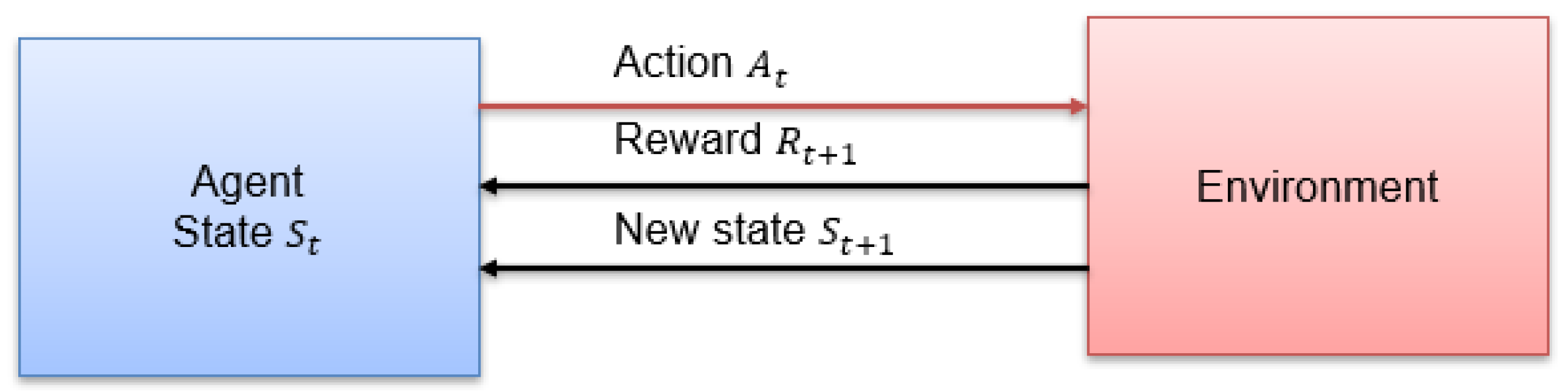
4.1. The MDP Model
- State and Action Spaces
- State Space (S)
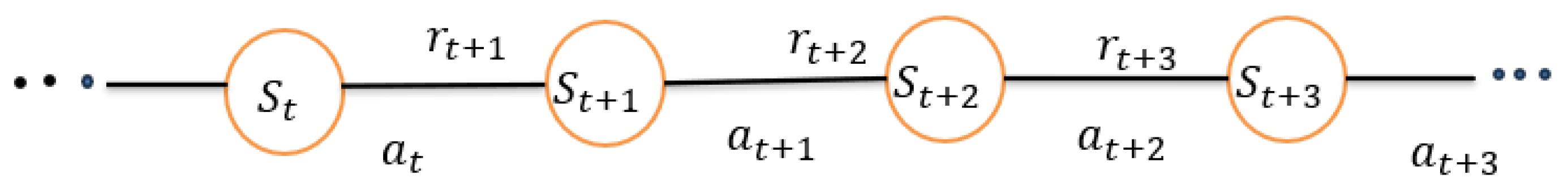
- Step 1: ; action , is taken and estimated reward is obtained.
- Step 2: ; action , is taken and estimated reward is obtained.
- Step 3: ; action , is taken and estimated reward is obtained.
- Step 4: ; action , is taken and estimated reward is obtained.
- Step 5: ; cumulative reward R, is obtained after completing one iteration.
- Action (A)
- State Transition
4.2. Immediate Reward
- denotes the UAV’s travel time from state to .
- represents the UAV’s communication time (data collection and sensor recharging) at state .
- is the deadline associated with state .
- P is a penalty for any constraint violations.
- Immediate Reward Calculations
4.3. DQN-Based UAV Detouring Algorithm
| Algorithm 1 DQN-based UAV detouring Algorithm |
| Input: Set of sensors Output: A detour traveling path of UAV with minimum total energy consumption
|
5. Performance Evaluation
5.1. Experimental Settings
5.2. Description of the Compared Algorithms
5.2.1. DQN-Based UAV Detouring Algorithm with a Negative Reward
5.2.2. The Greedy Algorithm
5.2.3. The Genetic Algorithm (GA)
5.2.4. Ant Colony Optimization (ACO) Algorithm
5.3. Performance Comparison Between the Proposed DQN-Based UAV Detouring Algorithm with a Negative Reward
5.4. Training Efficiency of the DQN-Based Detouring Algorithm
5.5. Performance Comparison Between the DQN-Based UAV Detouring Algorithm and Other Baseline Algorithms
6. Concluding Remarks
Author Contributions
Funding
Data Availability Statement
Conflicts of Interest
References
- Gao, H.; Feng, J.; Xiao, Y.; Zhang, B.; Wang, W. A uav-assisted multi-task allocation method for mobile crowd sensing. IEEE Trans. Mob. Comput. 2022, 22, 3790–3804. [Google Scholar] [CrossRef]
- Zhan, C.; Zeng, Y.; Zhang, R. Energy-efficient data collection in uav enabled wireless sensor network. IEEE Wirel. Commun. Lett. 2017, 7, 328–331. [Google Scholar] [CrossRef]
- Messaoudi, K.; Oubbati, O.S.; Rachedi, A.; Lakas, A.; Bendouma, T.; Chaib, N. A survey of uav-based data collection: Challenges, solutions and future perspectives. J. Netw. Comput. Appl. 2023, 216, 103670. [Google Scholar] [CrossRef]
- Rahman, S.; Akter, S.; Yoon, S. Oadc: An obstacle-avoidance data collection scheme using multiple unmanned aerial vehicles. Appl. Sci. 2022, 12, 11509. [Google Scholar] [CrossRef]
- Wu, P.; Xiao, F.; Sha, C.; Huang, H.; Sun, L. Trajectory optimization for UAVs’ efficient charging in wireless rechargeable sensor networks. IEEE Trans. Veh. Technol. 2020, 69, 4207–4220. [Google Scholar] [CrossRef]
- Baek, J.; Han, S.I.; Han, Y. Optimal uav route in wireless charging sensor networks. IEEE Internet Things J. 2019, 7, 1327–1335. [Google Scholar] [CrossRef]
- Rahman, S.; Akter, S.; Yoon, S. Energy-efficient charging of sensors for uav-aided wireless sensor network. Int. J. Internet Broadcast. Commun. 2022, 14, 80–87. [Google Scholar]
- Nazib, R.A.; Moh, S. Energy-efficient and fast data collection in uav-aided wireless sensor networks for hilly terrains. IEEE Access 2021, 9, 23168–23190. [Google Scholar] [CrossRef]
- Say, S.; Inata, H.; Liu, J.; Shimamoto, S. Priority-based data gathering framework in uav-assisted wireless sensor networks. IEEE Sensors J. 2016, 16, 5785–5794. [Google Scholar] [CrossRef]
- Samir, M.; Sharafeddine, S.; Assi, C.M.; Nguyen, T.M.; Ghrayeb, A. Uav trajectory planning for data collection from time-constrained iot devices. IEEE Trans. Wirel. Commun. 2019, 19, 34–46. [Google Scholar] [CrossRef]
- Ebrahimi, D.; Sharafeddine, S.; Ho, P.-H.; Assi, C. Uav-aided projection-based compressive data gathering in wireless sensor networks. IEEE Internet Things J. 2018, 6, 1893–1905. [Google Scholar] [CrossRef]
- Dong, M.; Ota, K.; Lin, M.; Tang, Z.; Du, S.; Zhu, H. Uav-assisted data gathering in wireless sensor networks. J. Supercomput. 2014, 70, 1142–1155. [Google Scholar] [CrossRef]
- Cao, H.; Liu, Y.; Yue, X.; Zhu, W. Cloud-assisted uav data collection for multiple emerging events in distributed wsns. Sensors 2017, 17, 1818. [Google Scholar] [CrossRef]
- Alfattani, S.; Jaafar, W.; Yanikomeroglu, H.; Yongacoglu, A. Multi-uav data collection framework for wireless sensor networks. In Proceedings of the 2019 IEEE Global Communications Conference (GLOBECOM), Waikoloa, HI, USA, 9–13 December 2019; pp. 1–6. [Google Scholar]
- Binol, H.; Bulut, E.; Akkaya, K.; Guvenc, I. Time optimal multi-uav path planning for gathering its data from roadside units. In Proceedings of the 2018 IEEE 88th Vehicular Technology Conference (VTC-Fall), Chicago, IL, USA, 27–30 August 2018; pp. 1–5. [Google Scholar]
- Raj, P.P.; Khedr, A.M.; Aghbari, Z.A. Edgo: Uav-based effective data gathering scheme for wireless sensor networks with obstacles. Wirel. Netw. 2022, 28, 2499–2518. [Google Scholar]
- Wang, X.; Gursoy, M.C.; Erpek, T.; Sagduyu, Y.E. Learning-based uav path planning for data collection with integrated collision avoidance. IEEE Internet Things J. 2022, 9, 16663–16676. [Google Scholar] [CrossRef]
- Poudel, S.; Moh, S. Hybrid path planning for efficient data collection in uav-aided wsns for emergency applications. Sensors 2021, 21, 2839. [Google Scholar] [CrossRef] [PubMed]
- Ghdiri, O.; Jaafar, W.; Alfattani, S.; Abderrazak, J.B.; Yanikomeroglu, H. Offline and online uav-enabled data collection in time-constrained iot networks. IEEE Trans. Green Commun. Netw. 2021, 5, 1918–1933. [Google Scholar] [CrossRef]
- Bouhamed, O.; Ghazzai, H.; Besbes, H.; Massoud, Y. A uav-assisted data collection for wireless sensor networks: Autonomous navigation and scheduling. IEEE Access 2020, 8, 110446–110460. [Google Scholar] [CrossRef]
- Wu, Y.; Song, W.; Cao, Z.; Zhang, J.; Lim, A. Learning improvement heuristics for solving routing problems. IEEE Trans. Neural Netw. Learn. Syst. 2021, 33, 5057–5069. [Google Scholar] [CrossRef] [PubMed]
- Bogyrbayeva, A.; Yoon, T.; Ko, H.; Lim, S.; Yun, H.; Kwon, C. A deep reinforcement learning approach for solving the traveling salesman problem with drone. Transp. Res. Part C Emerg. Technol. 2023, 148, 103981. [Google Scholar] [CrossRef]
- Kim, M.; Park, J. Learning collaborative policies to solve np-hard routing problems. Adv. Neural Inf. Process. Syst. 2021, 34, 10418–10430. [Google Scholar]
- Deudon, M.; Cournut, P.; Lacoste, A.; Adulyasak, Y.; Rousseau, L.-M. Learning heuristics for the tsp by policy gradient. In Integration of Constraint Programming, Artificial Intelligence, and Operations Research: 15th International Conference, CPAIOR 2018, Delft, The Netherlands, 26–29 June 2018; Proceedings 15; Springer: Cham, Switzerland, 2018; pp. 170–181. [Google Scholar]
- Pan, X.; Jin, Y.; Ding, Y.; Feng, M.; Zhao, L.; Song, L.; Bian, J. H-tsp: Hierarchically solving the large-scale traveling salesman problem. In Proceedings of the AAAI Conference on Artificial Intelligence, Washington, DC, USA, 7–14 February 2023; Volume 37, pp. 9345–9353. [Google Scholar]
- Malazgirt, G.A.; Unsal, O.S.; Kestelman, A.C. Tauriel: Targeting traveling salesman problem with a deep reinforcement learning inspired architecture. arXiv 2019, arXiv:1905.05567. [Google Scholar]
- Sui, J.; Ding, S.; Liu, R.; Xu, L.; Bu, D. Learning 3-opt heuristics for traveling salesman problem via deep reinforcement learning. In Proceedings of the Asian Conference on Machine Learning, PMLR, Virtual, 17–19 November 2021; pp. 1301–1316. [Google Scholar]
- Costa, P.R.d.O.; Rhuggenaath, J.; Zhang, Y.; Akcay, A. Learning 2-opt heuristics for the traveling salesman problem via deep reinforcement learning. In Proceedings of the Asian Conference on Machine Learning, PMLR, Bangkok, Thailand, 18–20 November 2020; pp. 465–480. [Google Scholar]
- Alharbi, M.G.; Stohy, A.; Elhenawy, M.; Masoud, M.; Khalifa, H.A.E.-W. Solving pickup and drop-off problem using hybrid pointer networks with deep reinforcement learning. PLoS ONE 2022, 17, e0267199. [Google Scholar] [CrossRef] [PubMed]
- Zhang, R.; Prokhorchuk, A.; Dauwels, J. Deep reinforcement learning for traveling salesman problem with time windows and rejections. In Proceedings of the 2020 International Joint Conference on Neural Networks (IJCNN), Glasgow, UK, 19–24 July 2020; pp. 1–8. [Google Scholar]
- Zhu, B.; Bedeer, E.; Nguyen, H.H.; Barton, R.; Henry, J. Uav trajectory planning in wireless sensor networks for energy consumption minimization by deep reinforcement learning. IEEE Trans. Veh. Technol. 2021, 70, 9540–9554. [Google Scholar] [CrossRef]
- Mao, X.; Wu, G.; Fan, M.; Cao, Z.; Pedrycz, W. Dl-drl: A double-level deep reinforcement learning approach for large-scale task scheduling of multi-uav. IEEE Trans. Autom. Sci. Eng. 2024. [Google Scholar] [CrossRef]
- Zhang, S.; Li, Y.; Dong, Q. Autonomous navigation of uav in multi-obstacle environments based on a deep reinforcement learning approach. Appl. Soft Comput. 2022, 115, 108194. [Google Scholar] [CrossRef]
- Su, X.; Ren, Y.; Cai, Z.; Liang, Y.; Guo, L. A q-learning based routing approach for energy efficient information transmission in wireless sensor network. IEEE Trans. Netw. Serv. Manag. 2022, 20, 1949–1961. [Google Scholar] [CrossRef]
- Liu, Y.; Yan, J.; Zhao, X. Deep-reinforcement-learning-based optimal transmission policies for opportunistic uav-aided wireless sensor network. IEEE Internet Things J. 2022, 9, 13823–13836. [Google Scholar] [CrossRef]
- Emami, Y.; Wei, B.; Li, K.; Ni, W.; Tovar, E. Joint communication scheduling and velocity control in multi-uav-assisted sensor networks: A deep reinforcement learning approach. IEEE Trans. Veh. Technol. 2021, 70, 10986–10998. [Google Scholar] [CrossRef]
- Luo, X.; Chen, C.; Zeng, C.; Li, C.; Xu, J.; Gong, S. Deep reinforcement learning for joint trajectory planning, transmission scheduling, and access control in uav-assisted wireless sensor networks. Sensors 2023, 23, 4691. [Google Scholar] [CrossRef]
- Yi, M.; Wang, X.; Liu, J.; Zhang, Y.; Bai, B. Deep reinforcement learning for fresh data collection in uav-assisted iot networks. In Proceedings of the IEEE INFOCOM 2020-IEEE Conference on Computer Communications Workshops (INFOCOM WKSHPS), Toronto, ON, Canada, 6–9 July 2020; pp. 716–721. [Google Scholar]
- Li, K.; Ni, W.; Tovar, E.; Guizani, M. Deep reinforcement learning for real-time trajectory planning in uav networks. In Proceedings of the 2020 International Wireless Communications and Mobile Computing (IWCMC), Limassol, Cyprus, 15–19 June 2020; pp. 958–963. [Google Scholar]
- Zhang, N.; Liu, J.; Xie, L.; Tong, P. A deep reinforcement learning approach to energy-harvesting uav-aided data collection. In Proceedings of the 2020 International Conference on Wireless Communications and Signal Processing (WCSP), Nanjing, China, 21–23 October 2020; pp. 93–98. [Google Scholar]
- Oubbati, O.S.; Lakas, A.; Guizani, M. Multiagent deep reinforcement learning for wireless-powered uav networks. IEEE Internet Things J. 2022, 9, 16044–16059. [Google Scholar] [CrossRef]
- Li, K.; Ni, W.; Dressler, F. Lstm-characterized deep reinforcement learning for continuous flight control and resource allocation in uav-assisted sensor network. IEEE Internet Things J. 2021, 9, 4179–4189. [Google Scholar] [CrossRef]
- Hu, Y.; Liu, Y.; Kaushik, A.; Masouros, C.; Thompson, J.S. Timely data collection for uav-based iot networks: A deep reinforcement learning approach. IEEE Sens. J. 2023, 23, 12295–12308. [Google Scholar] [CrossRef]
- Emami, Y.; Wei, B.; Li, K.; Ni, W.; Tovar, E. Deep q-networks for aerial data collection in multi-uav-assisted wireless sensor networks. In Proceedings of the 2021 International Wireless Communications and Mobile Computing (IWCMC), Harbin, China, 28 June–2 July 2021; pp. 669–674. [Google Scholar]
- Guo, Z.; Chen, H.; Li, S. Deep reinforcement learning-based uav path planning for energy-efficient multitier cooperative computing in wireless sensor networks. J. Sens. 2023, 2023, 2804943. [Google Scholar] [CrossRef]
- Kurs, A.; Karalis, A.; Moffatt, R.; Joannopoulos, J.D.; Fisher, P.; Soljacic, M. Wireless power transfer via strongly coupled magnetic resonances. Science 2007, 317, 83–86. [Google Scholar] [CrossRef] [PubMed]
- Liu, H.; Chu, X.; Leung, Y.-W.; Du, R. Minimum-cost sensor placement for required lifetime in wireless sensor-target surveillance networks. IEEE Trans. Parallel Distrib. Syst. 2012, 24, 1783–1796. [Google Scholar] [CrossRef]
- Sutton, R.S.; Barto, A.G. Reinforcement Learning: An Introduction; MIT Press: Cambridge, MA, USA, 2018. [Google Scholar]
- Akter, S.; Dao, T.-N.; Yoon, S. Time-constrained task allocation and worker routing in mobile crowd-sensing using a decomposition technique and deep q-learning. IEEE Access 2021, 9, 95808–95822. [Google Scholar] [CrossRef]
- Dorigo, M.; Birattari, M.; Stutzle, T. Ant colony optimization. IEEE Comput. Intell. Mag. 2006, 1, 28–39. [Google Scholar] [CrossRef]


| Study Reference | Proposed Algorithm | Original TSP Problem | Considered Problem | Objectives | Considered Constraints | Obstacles Existence |
|---|---|---|---|---|---|---|
| proposed work | proposed DQN-based UAV detouring algorithm | increment of TSP tour as obstacles have been considered in the TSP tour | proposed DOCEM problem | minimize total energy consumption of UAV | UAV’s travel deadline and energy constraints, sensors’ individual deadlines and residual energy constraints | Yes |
| [21] | deep reinforcement learning | Yes | routing problems | improvement heuristics for routing problems | No | No |
| [33] | deep reinforcement learning | Yes | autonomous navigation of UAV | reduce the reality gap and analyze UAV behaviors | No | Yes |
| [34] | Q learning | Yes | transmission Routing | reduce and balance the energy consumption of wireless sensors | No | No |
| [42] | deep reinforcement learning | No | Continuous Flight Control and Resource Allocation | minimize the overall data loss of the ground devices | No | No |
| [43] | deep reinforcement learning | No | Efficient data collection | maximizing the number of collected nodes | No | No |
| [44] | deep Q-Network | No | Optimal ground sensor selection at UAVs | minimize data packet losses | No | No |
| Notation | Definition |
|---|---|
| number of sensors | |
| number of obstacles | |
| set of sensors, | |
| set of obstacles, | |
| UAV battery capacity | |
| UAV communication time | |
| Arrival deadline for UAV at each sensor j | |
| Energy transfer efficiency when UAV recharges a sensor | |
| UAV’s flight speed | |
| UAV’s power level at full speed | |
| Energy consumption for generating one bit of data | |
| Energy usage per bit transmitted | |
| Energy transfer rate from UAV to a sensor while collecting data | |
| Energy transfer rate from UAV to sensor while recharging it | |
| Data generation rate of the sensor | |
| D | Deadline for data delivery to the sink for one UAV tour |
| a sensor–obstacle relationship matrix to define the relationships between sensors and the obstacles between them |
| Parameters | Values |
|---|---|
| Area size | |
| Number of sensors, n | 5, 10, 15, 20, 25, 30 |
| Number of obstacles, s | |
| Velocity of the UAV, | 55 |
| Deadline for data delivery to the sink for one tour, | 25 [4] |
| UAV’s power level at full speed, | 5 [31] |
| UAV’s power level when it hovers, | 0 [31] |
| UAV communication time, | 2 [4] |
| UAV battery capacity, | 50 × 104 [49] |
| UAV Arrival deadlines, | |
| Energy transfer efficiency, | 40% [46] |
| Energy consumption to generate one bit of data, | 50 [47] |
| Energy usage per bit of transmission electronics, | 50 [47] |
| Energy transfer rate from UAV to sensor i while collecting data from sensor i, | 5 |
| Energy usage per bit of transmission electronics, | 5 |
| Energy transfer rate from UAV to sensor i while charging, | 10 |
| Data generation rate of sensor, | 0.5 [47] |
| Size of the data | 64 bytes or 512 bits [47] |
| Parameters | Values |
|---|---|
| Total episodes | 7000 |
| Number of steps for Q-learning | 3 |
| Learning rate | |
| Discount factor | |
| Learning decay rate | 0.00001–2 |
| Epsilon min | 0.1 |
| Epsilon decay rate | 0 0.0006 |
| Memory buffer | 10,000 |
| Batch size | 16 |
| Optimizer | Adam |
Disclaimer/Publisher’s Note: The statements, opinions and data contained in all publications are solely those of the individual author(s) and contributor(s) and not of MDPI and/or the editor(s). MDPI and/or the editor(s) disclaim responsibility for any injury to people or property resulting from any ideas, methods, instructions or products referred to in the content. |
© 2024 by the authors. Licensee MDPI, Basel, Switzerland. This article is an open access article distributed under the terms and conditions of the Creative Commons Attribution (CC BY) license (https://creativecommons.org/licenses/by/4.0/).
Share and Cite
Rahman, S.; Akter, S.; Yoon, S. A Deep Q-Learning Based UAV Detouring Algorithm in a Constrained Wireless Sensor Network Environment. Electronics 2025, 14, 1. https://doi.org/10.3390/electronics14010001
Rahman S, Akter S, Yoon S. A Deep Q-Learning Based UAV Detouring Algorithm in a Constrained Wireless Sensor Network Environment. Electronics. 2025; 14(1):1. https://doi.org/10.3390/electronics14010001
Chicago/Turabian StyleRahman, Shakila, Shathee Akter, and Seokhoon Yoon. 2025. "A Deep Q-Learning Based UAV Detouring Algorithm in a Constrained Wireless Sensor Network Environment" Electronics 14, no. 1: 1. https://doi.org/10.3390/electronics14010001
APA StyleRahman, S., Akter, S., & Yoon, S. (2025). A Deep Q-Learning Based UAV Detouring Algorithm in a Constrained Wireless Sensor Network Environment. Electronics, 14(1), 1. https://doi.org/10.3390/electronics14010001