Adaptive Dynamic Boundary Sliding Mode Control for Robotic Manipulators under Varying Disturbances

Abstract

This paper introduces an Adaptive Dynamic Bounded Sliding Mode Control (ADBSMC) method that incorporates a disturbance observer to enhance the response characteristics of the robot manipulator while eliminating the reliance on a priori knowledge. The proposed method utilizes nonlinear sliding mode manifolds and fast-terminal-type convergence laws to address errors and parameter uncertainties inherent in the nonlinear system models. The adaptive law is designed to cover all boundary conditions based on the model’s state. It can dynamically determine upper and lower bounds without requiring prior knowledge. Consequently, the ADBSMC control method amalgamates the benefits of adaptive law and fast terminal sliding mode, leading to significant enhancements in control performance compared with traditional sliding mode control (SMC), exhibiting robustness against uncertain disturbances. To mitigate external disturbances, a system-adapted disturbance observer is devised, facilitating real-time monitoring and compensation for system disturbances. The stability of ADBSMC is demonstrated through the Lyapunov method. Simulation and experimental results validate the effectiveness and superiority of the ADBSMC control scheme, showcasing its potential for practical applications.

1. Introduction

Robot manipulators have been widely used in industrial processes for a variety of high-precision and complex work scenarios, such as industrial production lines, machine tool loading and unloading, palletizing, machining, and welding [1]. In order to cope with the requirements of different types of tasks, the tracking capabilities of robotic manipulators have to be more precise and faster. Although there have been some studies on the control functions of robotic arms, some problems may arise when designing the control algorithms, such as errors and parameter uncertainties [2] between the nonlinear system and the modeled system, some parameters of the system itself which may require some a priori knowledge [3] to determine their ranges, or some external factors, for example, noise, friction and collision may occur, which can create a time-varying perturbations [4]. These factors may make the robotic arm movement inaccurate or even cause instability of the overall system.

Commonly used control methods for robotic arms include sliding mode control [5], PID control [6], and neural network control [7]. Sliding mode control (SMC) has the advantage of being insensitive to system uncertainty and parameter changes, which can somewhat solve the instability factors that may occur in the robotic arm system. By using Matlab, we can simulate the movement path of the robotic arm more easily [8]. Among them, Ilgenl et al. [9] optimized the SMC controller by using the Simple Shape Search (SS) method and used it in controlling the trajectory tracking of a two-link planar robot manipulator arm, which has been shown experimentally to exhibit effective control performance in terms of trajectory, stabilization time, and end position required by the system. Ahmed et al. [10] applied a new sliding mode control with PD and fuzzy control in the antishudder control of robot manipulator. The effectiveness and efficiency of the proposed control method is experimentally verified. Ji et al. [11] proposed an improved exponential convergence law and nonlinear sliding mode surface for the problems of convergence speed and shuddering in the sliding mode variable structure control of manipulators. Experiments showed that it can improve the tracking accuracy and convergence speed to some extent while reducing system chattering. Sliding mode control applied to robotic arm control can improve its control accuracy, but due to the characteristics of its own algorithm, it is prone to high-frequency chattering, which in turn will produce noise, wear and tear, and other problems. At the same time, some parameters of the control algorithm need certain a priori knowledge to be defined, so it is necessary to make certain improvements to the sliding mode control algorithm.

There are many ways to improve the sliding mode control algorithm, such as neural network methods [12], data-driven MPC algorithms [13], and adaptive methods [14], among which the adaptive method is also one of the improvement methods. It has the advantages of high adaptability to parameter changes and high fault tolerance. It is usually divided into ascending–descending ASMC [15] and equivalent ASMC control [16]. For example, Zhao et al. [17] used the adaptive sliding film method to control the Dobot magician robotic arm and found that it has better self-tuning and trajectory tracking capabilities. Zaare et al. [18] presented a high-speed and low power consumption adaptive fuzzy global coupled nonsingular fast terminal sliding mode control to the position tracking control of the n-rigid-link elastic-joint robot manipulators in the presence of the uncertainties. Seung-Hun et al. [19] suggested an adaptive sliding mode control by using Nussbaum functions for the n-degree-of-freedom robotic arm tracking control problem. The experiment proved that the method can reduce the possibility of damage to the robotic arm when the control direction is uncertain. The adaptive method has, to some extent, enhanced the sensitivity of the sliding mode control to external disturbances, yet its capability to counteract time-varying external disturbances remains suboptimal. This indicates that the adaptive control approach requires further refinement. Recently, other researchers have also been making continuous improvements to adaptive control methods. For instance, Jerbi et al. [20] have developed an adaptive robust controller based on Radial Basis Function (RBF) neural network (NN) systems and the Hamilton–Jacobi–Isaacs (HJI) approach, which exhibits a commendable disturbance rejection performance in Wearable Robotic Knees (WRKs).

In response to the above problems, perturbation observers can significantly ameliorate the effects of complex external disturbances. For example, Yin et al. [21] used an adopted sliding film control based on a nonlinear disturbance observer for the tracking accuracy and disturbance immunity requirements of the trajectory tracking control of machining robot manipulators. Shi et al. [22] applied a fixed-time sliding mode control strategy based on an adaptive disturbance observer to the trajectory tracking control of a nonlinear robotic arm system and proved to be able to overcome the problem well. It was verified that it can well overcome the problems of modeling error, unknown perturbation, and friction in practical control. Juan Xian et al. [23] proposed a continuous sliding mode control scheme based on time-varying perturbation estimation and compensation in the study of high-precision trajectory tracking problem of uncertain robot manipulator arm, which has found that the scheme not only alleviates the jittery vibration but also makes the whole system’s antidisturbance performance significantly improved. In addition, Alshammari et al. [24] used fuzzy theory to establish two fuzzy switching manifolds on disturbance and slip film observer systems to improve the synthesis effect of the controller. Kchaou et al. [25] designed a set of slip film observer strategies based on fault-tolerant control with Takagi–Sugeno (T-S) fuzzy, which can be well-suited for nonlinear descriptor systems with actuator faults. Compared with the traditional sliding mode control, the adaptive sliding mode control with disturbance observer has a better control effect in terms of parameter uncertainty and complex disturbance.

In this paper, a terminal adaptive sliding mode control algorithm based on a disturbance observer is used to control a robotic arm. Firstly, the sliding mode control is utilized to cope with some error situations and parameter uncertainty that may be brought by the nonlinear model of the system. Secondly, an adaptive algorithm optimization is incorporated to cover all the boundary conditions by relying on the state of the model to be able to determine the corresponding, non-pre-fixed upper and lower bounds without the need for a priori knowledge. Finally, in order to cope with external interference, an interference observer is added, which can monitor and compensate for system interference in real time to ensure the stability and reliability of the overall system. Through the above algorithm design, the problems that may occur during the control of the seven-axis redundant robotic arm mentioned in the previous section can be better solved.

The rest of the paper is organized as follows. Section 2 describes the dynamics modeling of the robotic manipulator. Section 3 gives the design steps for the perturbation observer to be used. Section 4 designs the terminal adaptive sliding mode controller and performs stability analysis. Simulation and experimental results are given in Section 5 and Section 6. Finally, Section 7 gives the conclusions and outlook.

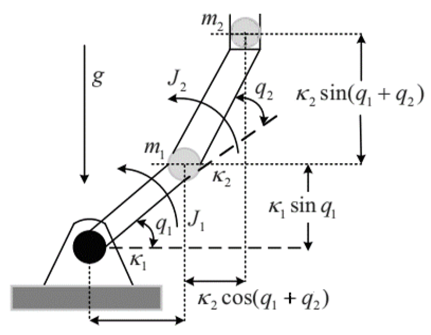
2. Dynamic Modeling

The dynamics of an n-link robot manipulator can be encapsulated by the following equation:

$$M\left(q\right)\ddot{q}+B(q,\dot{q})\dot{q}+G\left(q\right)=\tau +\xi$$

(1)

where $q\in {\mathbb{R}}^n$, $\dot{q}\in {\mathbb{R}}^n$, and $\ddot{q}\in {\mathbb{R}}^n$ are the vectors denoting the joint positions, velocities, and accelerations, respectively. The term $\tau \in {\mathbb{R}}^{n\times 1}$ signifies the control input torques. The matrix $M\left(q\right)\in {\mathbb{R}}^{n\times n}$ is the inertia matrix, portraying the mass properties of the manipulator. $B(q,\dot{q})\in {\mathbb{R}}^{n\times n}$ represents the Coriolis and centrifugal forces matrix, and $G\left(q\right)\in {\mathbb{R}}^{n\times 1}$ corresponds to the gravitational force matrix. Here, $M,B,G,\xi$, and their corresponding boundaries $\underline{m},\overline{m},\overline{b},\overline{g},\overline{\xi }$ are all considered unknown. The vector $\xi$ encompasses the total unknown disturbances in the system, including external disturbances and modeling errors.

A few assumptions are made here:

Assumption 1.

The robotic arm system expects the joint angular positions and angular velocities to be known, and the actual positions and velocity trajectories of the system and the first-order derivatives to be measurable and continuously bounded.

Assumption 2.

The total unknown disturbance ξ is assumed to be continuously differentiable and bounded, specifically $\left|\right|\dot{\xi }\left|\right|\le {\dot{Z}}_{\xi }$, where ${\dot{Z}}_{\xi }={[{\dot{Z}}_{{\xi }_1},{\dot{Z}}_{{\xi }_2},\dots ,{\dot{Z}}_{{\xi }_n}]}^T\in {\mathbb{R}}^n$ represents the upper bound of its first derivative.

The dynamic model adheres to several key properties:

Property 1.

The matrix $M\left(q\right)$ is a symmetric positive definite matrix and $\exists \underline{m},\overline{m}\in R^{+}$ such that $0<\underline{m}I\le M\left(q\right)\le \overline{m}I$.

Property 2.

$\exists \overline{b},\overline{g},\overline{d}\in R^{+}$ such that $\forall \ge 0,\left|\right|B(q,\dot{q})\left|\right|\le \overline{b}\left|\right|\dot{q}\left|\right|,\left|\right|G\left(q\right)\left|\right|\le \overline{g},\left|\right|\xi \left(t\right)\left|\right||\le \overline{\xi }$.

Property 3.

$\dot{M}\left(q\right)-2B(q,\dot{q})$ is skew-symmetric. For brevity, q and $\dot{q}$ are often omitted in $M\left(q\right)$, $B(q,\dot{q})$, and $G\left(q\right)$. And it is satisfied with $z^T(\dot{M}\left(q\right)-2B(q,\dot{q}))z=0$ for any nonzero vector z.

To further elucidate the dynamics of the robotic manipulator, the state–space representation of the dynamic equation is presented as follows:

$$\left\{\begin{array}{cc}{\dot{x}}_1=x_2\hfill & \\ {\dot{x}}_2=M^{-1}(\tau -B(x_1,x_2)x_2-G\left(x_1\right))+M^{-1}\xi \hfill & \\ y=x_1\hfill \end{array}\right.$$

(2)

The goal of the control method proposed in this study is to establish a control law in the form of actuator torque in the presence of disturbances and uncertainties that ensures that the joint output angle q accurately follows the desired joint trajectory $q_d$.

3. Disturbance Observer Design

As the manipulator arm has external disturbances and its own modeling uncertainty in the actual control process, this will reduce the control accuracy of the manipulator arm. In order to reduce the influence of external disturbances on the robotic arm system, a disturbance observer is designed in this section in conjunction with the robotic arm dynamics model, which is used to approximate the system disturbance and differentiate them from the actual disturbances, and the disturbance error is converged to zero by correcting the disturbance estimate.

Based on the Equation (2), the perturbation observer of the manipulator arm is designed as:

$$\dot{\widehat{\xi }}=L\left(x_1\right)(M\left(x_1\right){\dot{x}}_2+B(x_1,x_2)x_2+G\left(x_1\right)-\tau -\widehat{\xi })$$

(3)

where $L\left(x_1\right)=diag(l_{11},l_{12},\dots ,l_{1n})>0$ is the nonlinear gain matrix and $\widehat{\xi }$ is the observed estimate of $\xi$.

Since the above equation needs to realize the angular acceleration of the state, using the velocity signal differentiation to obtain the acceleration signal will introduce noise leading to system instability. So, to solve the above problem, the interference observer can be designed as follows. Construct the following auxiliary function:

$$\zeta =\widehat{\xi }-p\left(x_1\right)$$

(4)

where $p\left(x_1\right)={\int }_0^{t}L\left(x_1\right)x_{1}dt$. $\zeta \in R^n$ is the internal state vector of the observer, $p\left(x_1\right)\in R^n$ is the vector of the function yet to be designed, and in order to avoid the introduction of acceleration signals, the perturbation of observer gain matrix $L\left(x_1\right)$ and $p\left(x_1\right)$ exists in the following relationship:

$$L\left(x_1\right)M\left(x_1\right){\dot{x}}_2=\frac{dp\left(x_1\right)}{d{x}_1}$$

(5)

Based on Equations (3)–(5), the structure of the interference observer can be designed as:

$$\dot{\zeta }=L\left(x_1\right)(B(x_1,x_2)x_2+G\left(x_1\right)-\tau -\zeta -p\left(x_1\right))$$

(6)

Since a perturbed observer without acceleration is required, a modification of the above equation can be obtained:

$$\left\{\begin{array}{cc}\widehat{\xi }=\zeta +p\left(x_1\right)\hfill & \\ \dot{\zeta }=-L\left(x_1\right)\zeta +L\left(x_1\right)(B(x_1,x_2)x_2+G\left(x_1\right)-\tau -p\left(x_1\right))\hfill \end{array}\right.$$

(7)

After obtaining the non-accelerated perturbation observer, the observation error of the perturbation observer is defined as follows:

$$z=\xi -\widehat{\xi }$$

(8)

From Equations (4) to (8), the dynamic equation of the observer error is

$$\begin{array}{cc}\hfill \dot{z}& =\dot{\xi }-\dot{\widehat{\xi }}\hfill \\ & =\dot{\xi }-L\left(x_1\right)\xi +L\left(x_1\right)\widehat{\xi }\hfill \end{array}$$

(9)

The above equation requires a priori knowledge of interference differentiation, but this part of the actual conditions is unknown. Here, it is assumed that $\xi$ changes slowly with respect to the characteristics of the interference observer, so Equation (9) becomes as follows:

$$\dot{z}+L\left(x_1\right)z=0$$

(10)

In the equation, take the nonlinear gain matrix $L\left(x_1\right)={\tilde{\rho }}^{-1}{M}^{-1}\left(x_1\right),{\tilde{\rho }}^{-1}$ as an invertible matrix, and bring it into the integral of Equation (5) to obtain:

$$p\left(x_1\right)={\tilde{\rho }}^{-1}\dot{q}$$

(11)

In order to realize the accurate estimation of $\xi$ by adjusting $L\left(x\right)$ so that the disturbance observation $\widehat{\xi }$ approximates the total unknown disturbance $\xi$ so that the observer error z can converge to zero exponentially. To ensure the stability of the observer, the following Lyapunov function is constructed:

$$V_{DO}=z{\tilde{\rho }}^{T}M\left(x_1\right)\tilde{\rho }z$$

(12)

From Equation (10):

$$\left\{\begin{array}{cc}\dot{z}=-{\tilde{\rho }}^{-1}{M}^{-1}\left(x_1\right)z\hfill & \\ {\dot{z}}^T=-z^T{M}^{-T}\left(x_1\right){\tilde{\rho }}^{-1}\hfill \end{array}\right.$$

(13)

Then, the derivation and simplification of $V_{DO}$ is obtained:

$$\begin{array}{cc}\hfill {\dot{V}}_{DO}& =-z^T\tilde{\rho }z-z^T\tilde{\rho }z+z^T\tilde{\rho }\dot{M}\left(x_1\right){\tilde{\rho }}^{T}z\hfill \\ \hfill & =-z^T(\tilde{\rho }+{\tilde{\rho }}^T-\tilde{\rho }\dot{M}\left(x_1\right){\tilde{\rho }}^T)z\hfill \end{array}$$

(14)

Assume that there exists a symmetric positive definite matrix $\varpi >0$ such that $\tilde{\rho }+{\tilde{\rho }}^T-\tilde{\rho }\dot{M}\left(x_1\right){\tilde{\rho }}^T$ in Equation (14) satisfies:

$$\tilde{\rho }+{\tilde{\rho }}^T-\tilde{\rho }\dot{M}\left(x_1\right){\tilde{\rho }}^T\ge \varpi$$

(15)

By multiplying both sides of the Equation (15) with ${\tilde{\rho }}^{-T}$ and ${\tilde{\rho }}^{-1}$, respectively, we obtain

$${\tilde{\rho }}^{-T}+{\tilde{\rho }}^{-1}-{\tilde{\rho }}^{-T}\varpi {\tilde{\rho }}^{-1}\ge \dot{M}\left(x_1\right)$$

(16)

According to the Assumption 1, there exists a $\psi >0$ such that $\dot{M}\left(x_1\right)\le \psi I_n$, where $I_n$ is the identity matrix. Consequently, the Equation (16) becomes

$${\tilde{\rho }}^{-T}+{\tilde{\rho }}^{-1}-{\tilde{\rho }}^{-T}\varpi {\tilde{\rho }}^{-1}\ge 0$$

(17)

Finally, by applying the Schur complement theorem, Equation (17) is converted to the following matrix:

$$\left[\begin{array}{cc}{\tilde{\rho }}^{-T}+{\tilde{\rho }}^{-1}-\psi I_n& {\tilde{\rho }}^{-T}\\ {\tilde{\rho }}^{-1}& {\varpi }^{-1}\end{array}\right]\ge 0$$

(18)

Use the Linear Matrix Inequality (LMI) toolbox to solve Equation (18), thus ensuring that ${\dot{V}}_{DO}<0$ is negatively definite.

4. Controller Design

In this section, a set of adaptive-based terminal sliding mode controllers will be designed in order to satisfy its need for no a priori knowledge and no prefixed upper and lower bounds.

Before proceeding with the design of the sliding mold surface, it needs to specify the inputs to the system. The inputs to the system are the deviation values of the manipulator arm joint angles and angular velocities of the robotic arm, which can be expressed as

$$\left\{\begin{array}{cc}e\left(t\right)=q-q_d\hfill & \\ \dot{e}\left(t\right)=\dot{q}-{\dot{q}}_d\hfill & \end{array}\right.$$

(19)

To better represent the error vector, define $E={\left[e^T{\dot{e}}^T\right]}^T$. And $\left|\right|E\left|\right|\ge \left|\right|e\left|\right|,\left|\right|E\left|\right|\ge \left|\right|\dot{e}\left|\right|$.

Accordingly, the nonlinear fast terminal sliding mode surface function can be written as

$$s\left(t\right)=e+\alpha si{g}^{{\gamma }_1}\left(e\right)+\beta si{g}^{{\gamma }_2}\left(\dot{e}\right)$$

(20)

where $\alpha >0,\beta >0,{\gamma }_2=p/q$ and $p,q(p>q)$ are positive odd numbers satisfying $1<{\gamma }_2<2,{\gamma }_1>{\gamma }_2$; $si{g}^{\gamma }\left(e\right)$ is defined as $si{g}^{\gamma }\left(e\right)={\left|e\right|}^{\gamma }sign\left(e\right)$ and $\left|\right|\alpha si{g}^{{\gamma }_1}\left(e\right)|\le \alpha |\left|e\right||,||\beta si{g}^{{\gamma }_2}\left(\dot{e}\right)\left|\right|\le \beta \left|\right|\dot{e}\left|\right|$.

Derivation of the Equation (20) gives

$$\dot{s}\left(t\right)=\dot{e}+\alpha {\gamma }_1{\left|e\right|}^{{\gamma }_1-1}\dot{e}+\beta {\gamma }_2{\left|\dot{e}\right|}^{{\gamma }_2-1}\ddot{e}$$

(21)

To facilitate the next computational derivation process, multiplying M to the left of Equation (21) gives

$$\begin{array}{cc}\hfill M\dot{s}\left(t\right)& =M(\ddot{q}-{\ddot{q}}_d+\alpha {\gamma }_1|e{|}^{{\gamma }_1-1}\dot{e}+\beta {\gamma }_2\left|\dot{e}{|}^{{\gamma }_2-1}\ddot{e}\right)\hfill \\ & =\tau -Bs+\phi \hfill \end{array}$$

(22)

where $\phi =-[B\dot{q}+G-\xi +M{\ddot{q}}_d-M(\alpha {\gamma }_1{\left|e\right|}^{{\gamma }_1-1}\dot{e}+\beta {\gamma }_2|\dot{e}{|}^{{\gamma }_2-1}\ddot{e})-Bs]$.

Defined $\Gamma =\left|\right|{\ddot{q}}_d\left|\right|+\left|\right|\alpha {\gamma }_1{\left|e\right|}^{{\gamma }_1-1}\left|\right|·\left|\right|\dot{e}\left|\right|+\left|\right|\beta {\gamma }_2|\dot{e}{|}^{{\gamma }_2-1}\left|\right|·\left|\right|\ddot{e}\left|\right|$, $V=\left|\right|e\left|\right|+\left|\right|\alpha si{g}^{{\gamma }_1}\left(e\right)\left|\right|+\left|\right|\beta si{g}^{{\gamma }_2}\left(\dot{e}\right)\left|\right|$. From Properties 1 and 2, the range of $\phi$ in Equation (22) can be determined:

$$\begin{array}{cc}\hfill \left|\right|\phi \left|\right|& \le \overline{b}\left|\right|\dot{q}{\left|\right|}^2+\overline{g}+\overline{d}+\overline{m}\Gamma +\overline{b}\left|\right|\dot{q}\left|\right|V\hfill \\ \hfill & \le \overline{b}\left|\right|\dot{q}{\left|\right|}^2+\overline{g}+\overline{d}+\overline{m}\Gamma +\overline{b}\left|\right|\dot{q}\left|\right|\left(\right|\left|e\right||+\alpha \left|\right|e\left|\right|+\beta \left|\right|\dot{e}\left|\right|)\hfill \\ \hfill & \le \overline{b}\left|\right|\dot{q}{\left|\right|}^2+\overline{g}+\overline{d}+\overline{m}\left(\right||{\ddot{q}}_d\left|\right|+\left|\right|\alpha {\gamma }_1\left|\right|·\left|\right|\dot{e}\left|\right|+\left|\right|\beta {\gamma }_2\left|\right|·\left|\right|\ddot{e}\left|\right|)+\overline{b}\left|\right|\dot{q}\left|\right|\left(\right|\left|e\right||+\alpha \left|\right|e\left|\right|+\beta \left|\right|\dot{e}\left|\right|)\hfill \\ \hfill & \le \overline{b}\left|\right|\dot{q}{\left|\right|}^2+\overline{g}+\overline{d}+\overline{m}\left(\right||{\ddot{q}}_d\left|\right|+\left|\right|\alpha {\gamma }_1\left|\right|·\left|\right|\dot{e}\left|\right|)+\overline{b}\left|\right|\dot{q}\left|\right|\left(\right|\left|e\right||+\alpha \left|\right|e\left|\right|+\beta \left|\right|\dot{e}\left|\right|)\hfill \end{array}$$

(23)

Substituting Equation (19) into Equation (23) yields

$$\left|\right|\phi \left|\right|\le K_0^{\ast }+K_1^{\ast }\left|\right|E\left|\right|+K_2^{\ast }{\left|\right|E\left|\right|}^2$$

(24)

where $K_0^{\ast }=\overline{b}\left|\right|{\dot{q}}_d{\left|\right|}^2+\overline{g}+\overline{\xi }+\overline{m}\left|\right|{\ddot{q}}_d\left|\right|$, $K_1^{\ast }=\overline{b}\left|\right|{\dot{q}}_d\left|\right|(3+\left|\right|\alpha \left|\right|)+\overline{m}\left|\right|\alpha {\gamma }_1\left|\right|$, $K_2^{\ast }=\overline{b}\left|\right|{\dot{q}}_d\left|\right|(2+\left|\right|\beta \left|\right|)$ as the unknown boundary range.

According to the previous analysis and calculation, the control rate of fast terminal sliding mode control based on adaptive law can be obtained as

$${\tau }_{adp}=-cs-(k+\hslash \left(t\right))si{g}^n\left(s\right)$$

(25)

where $c>0,k>0,0<n<1$, and the adaptive law $\hslash \left(t\right)$ is defined as follows:

$$\hslash \left(t\right)={\widehat{K}}_0\left(t\right)+{\widehat{K}}_1\left(t\right)\left|\right|E\left|\right|+{\widehat{K}}_2{\left|\right|E\left|\right|}^2$$

(26)

$${\dot{\widehat{K}}}_i\left(t\right)={\left|\right|s\left(t\right)\left|\right|\left|\right|E\left|\right|}^i-{ϵ}_i{\widehat{K}}_i\left(t\right)$$

(27)

where ${\widehat{K}}_i\left(0\right)>0$, ${ϵ}_i>0$, ${ϵ}_i\in R^{+},i=0,1,2$. The control rate of the manipulator is as follows:

$$\tau ={\tau }_{eq}+{\tau }_{est}$$

(28)

The two control rates are, respectively,

$${\tau }_{eq}=M\left(q\right){\ddot{q}}_d+B(q,\dot{q})\dot{q}+G\left(q\right)-\widehat{\xi }$$

(29)

$${\tau }_{est}=-{\beta }^{-1}{\gamma }_2^{-1}M\left(q\right)(\alpha {\gamma }_1{\left|e\right|}^{{\gamma }_1-1}+1)·fa{l}^{2-{\gamma }_2}\left(\dot{e}\right)-M\left(q\right){\tau }_{adp}$$

(30)

where, to further attenuate the jitter, the power function $fal(s,\alpha ,\delta )$ is used instead of the $sig\left(s\right)$ function:

$$fal=\left\{\begin{array}{cc}{\left|s\right|}^{a}sign\left(s\right)\hfill & \\ s/{\delta }^{1-a}\hfill & \end{array}\right.$$

(31)

where $0<a<1$ is a constant that affects the tracking speed; $0<\delta <1$ is a constant that affects the filtering effect. The overall schematic diagram of the ADBSMC is depicted in Figure 1. The stability analysis is demonstrated in Appendix A.

5. Simulation

5.1. Simulation Setup

In order to demonstrate the effectiveness of our proposed ADBSMC controller, we performed two simulations using a 2-DOF robotic manipulator. The detail of the manipulator in Figure 2 is given as

$$\begin{array}{ccc}\hfill & M\left(q\right)=\left[\begin{array}{cc}{M}_{11}& M_{12}\\ M_{21}& M_{22}\end{array}\right],B(q,\dot{q})=\left[\begin{array}{cc}{B}_{11}& B_{12}\\ B_{21}& B_{22}\end{array}\right]\hfill & \\ \hfill & G\left(q\right)=\left[\begin{array}{c}{G}_{11}\\ G_{21}\end{array}\right],\tau \left(q\right)=\left[\begin{array}{c}{\tau }_1\\ {\tau }_2\end{array}\right]\hfill \end{array}$$

And, $M_{11}=(m_1+m_2)l_1^2+m_2{l}_2^2+2l_1{l}_2{m}_{2}cos{q}_2,$

$M_{12}=M_{21}=m_2{l}_2^2+m_2{l}_1{l}_{2}cos{q}_2,$

$M_{22}=l_2^2{m}_2+J_2,$

$B_{11}=-m_2{l}_1{l}_{2}sin\left(q_2\right){\dot{q}}_2,$

$B_{12}=-m_2{l}_1{l}_{2}sin\left(q_2\right){\dot{q}}_2({\dot{q}}_1+{\dot{q}}_2),$

$B_{21}=-m_2{l}_1{l}_{2}sin\left(q_2\right){\dot{q}}_1,$

$B_{22}=0,$

$G_{11}=(m_1{l}_2+m_2{l}_1)gcos\left(q_1\right)+m_2{l}_{2}gcos(q_1+q_2),$

$G_{21}=m_{2}g{l}_{2}cos(q_1+q_2)$.

where $m_{1,2}$ is the length of the manipulator, $l_{1,2}$ is the mass of the robotic arm, and $J_{1,2}$ is the inertia force. The parameters of the robotic manipulator are shown in

Table 1. The parameters of ADMSMC.

Parameter	Data	Parameter	Data
$\alpha$	$diag\{18,20\}$	$\beta$	$diag\{7,7\}$
a	$0.1$	$\delta$	$0.01$
c	$diag\{10,5\}$	k	$0.03$
${ϵ}_0$	18	$m_1$	1 kg
${ϵ}_1$	20	$m_2$	1 kg
${ϵ}_2$	22	$l_1$	0.4 m
$\tilde{\rho }$	$diag\{0.008,0.0047\}$	$l_2$	0.2 m
${\gamma }_1$	$1.1$	$J_1$	5 kg
${\gamma }_2$	$1.01$	$J_2$	5 kg

.

The expected motion trajectories adopted by joints 1 and 2 are $q_{1d}=cos(\pi t/12+\pi /2)$, $q_{2d}=sin(\pi t/12+\pi /2)$. The initial state of the manipulator is chosen as $\left[q_1{q}_2{\dot{q}}_1{\dot{q}}_2\right]=\left[10.100.1\right]$. The model uncertainty is set as $M_0=0.2M$, $B_0=0.2B$, $G_0=0.2G$. The control parameters of ADBSMC are shown in Table 1.

The proposed controller is compared with SMC, T2F−SFOSMC [26], and AISMC [27] to verify its superiority. In the first case, to illustrate the superiority of ADBSMC, a time-varying composite interference is added to the manipulator. The interference terms are $w_1=2·g·cos\left(q_1\right)+2·g·cos(q_1+q_2)$ and $w_2=2·g·cos(q_1+q_2)$. The second scenario is to suddenly add a disturbance of 15 Nm at the joint position of the manipulator at 1.3 s to demonstrate the robustness of our controller to unknown disturbances. For a fair comparison, the parameters of the sliding membrane part of the above controllers are all the same.

5.2. Simulation Results

5.2.1. Case One

In this case, the obtained results are presented in Figure 3, Figure 4 and Figure 5.

Figure 3a,c presents the tracking results of two robotic manipulator links under various control methods, while Figure 3b,d showcases the corresponding tracking errors. Notably, the ADBSMC method demonstrates superior adaptability to disturbances in the system. And the ADBSMC method consistently maintains the lowest error margins, particularly under conditions of higher disturbance, thereby affirming its efficacy in achieving precise control. While the conventional SMC, T2F−SFOSMC, and AISMC strategies exhibit satisfactory tracking, their performances are challenged under conditions of large disturbances. These methods are conventionally designed to address only small perturbations and thus falter when confronted with more substantial interference.

Figure 4 demonstrates the torque responses of a robotic manipulator under four different control strategies. The slight deviations present in the SMC and T2F−SFOSMC methods suggest a lower robustness against system uncertainties. In contrast, the AISMC and ADBSMC exhibit superior performance, with ADBSMC marginally outperforming AISMC by maintaining a consistent and smooth torque output.

Figure 5 displays the time history of adaptive law $\hslash \left(t\right)$. It was observed that the parameter $\hslash \left(t\right)$ remained continuous and free of chatter. Due to disparities between the actual and desired initial states of the manipulator, the parameter $\hslash \left(t\right)$ rapidly increased during the initial tracking phase to generate high-gain controls. Subsequently, $\hslash \left(t\right)$ adapted to the tracking error, ensuring continued excellent tracking performance.

5.2.2. Case Two

In this case, an external interference force was deliberately applied to the robotic manipulator, and the outcomes are depicted in Figure 6, Figure 7 and Figure 8.

Relative to Case One, we can find that the tracking accuracy of all controllers is significantly degraded when subjected to the impact disturbances in Figure 6. It is worth noting that the SMC strategy leads to a significant error. Compared with other methods, our method enables the error to converge to zero faster after being perturbed by shocks at the joints.

In Figure 7, the control inputs experienced an elevation in comparison with Case One, a phenomenon rationalized by the necessity for joints to augment torque to counteract the external payload.

Figure 8 displays that the adaptive parameter $\hslash \left(t\right)$ displayed an increase to ensure precise tracking. The discernible rise in control efforts is noteworthy, aligning with the imperative to mitigate the effects of the external disturbance.

To facilitate a rigorous comparison, we calculated the root mean square error (RMSE) and the maximum absolute error (MAE) for each case based on the simulated data, as detailed in

Table 2. Comparison of interference errors under simulation Case One and Case Two.

Controller	Random Disturbance		Impact and Random Disturbance
	Position	Position	Position	Position
	RMSE (rad)	MAE (rad)	RMSE (rad)	MAE (rad)
SMC	0.0357	0.0299	0.1774	0.0759
T2F−SFOSMC	0.0344	0.0320	0.0473	0.0380
AISMC	0.0165	0.0146	0.0192	0.0160
ADBSMC	0.0084	0.0033	0.0121	0.0080

.

Table 2 underscores that our proposed controller consistently maintains smaller RMSE and MAE values compared with the SMC, T2F−SFOSMC, and AISMC controllers, even under the influence of external disturbance. This reaffirms the robustness of our controller in achieving superior tracking performance in challenging conditions. Specifically, in Case One, the root mean square errors of the SMC, T2F−SFOSMC, and AISMC controllers are 0.0357, 0.0344, and 0.0165, respectively. The ADBSMC controller is the smallest with 0.0084. The same conclusion is reached in Case Two. Thus, the superiority of our proposed controller is proved.

6. Experiment

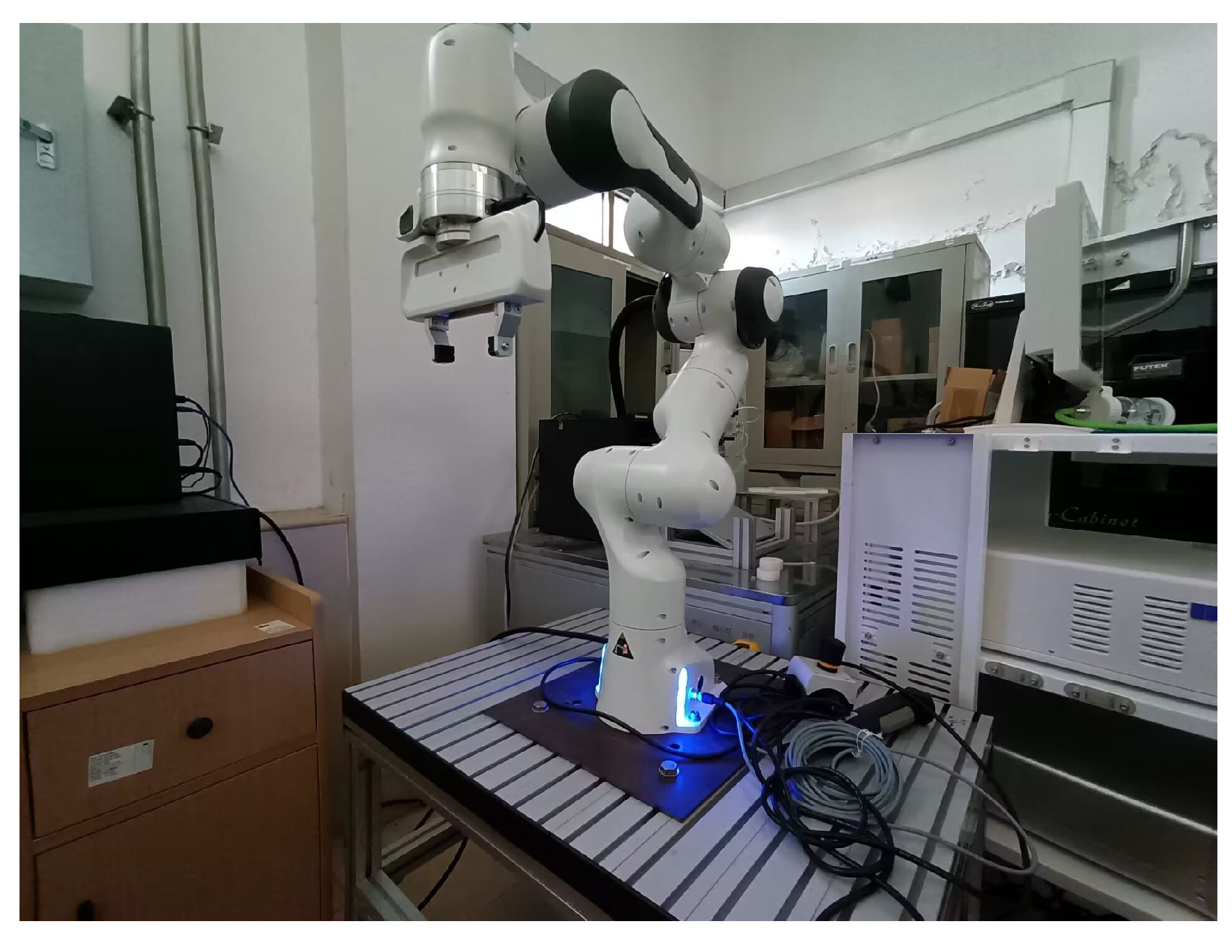
In order to verify the effectiveness of the proposed adaptive dynamic boundary sliding mode control based on the disturbance observer method in actual conditions, a comparative experimental study on the related tank is carried out in this section. As shown in Figure 9, the validation of the ADBSMC is demonstrated using a 7-DOF Franka–Emika–Panda robot equipped with high-precision torque sensors. Control of the robot is achieved through the Franka Control Interface (FCI), and real-time control values are transmitted at a frequency of 1 kHz [28]. The FCI provides a framework that enables the robot to receive real-time feedback from external sensors. The interface allows additional sensory information to be integrated into the robot’s control loop. The low-level control of the Franka is typically processed using C++. This involves direct communication with the robot’s hardware, real-time control loops, and handling low-level commands such as joint position control, torque control, and sensor data acquisition. We use Franka Matlab to create higher-level control logic. The FCI Simulink blocks send high-level commands to the robot, and then Simulink blocks translates into the appropriate low-level control signals that the robot recognises.

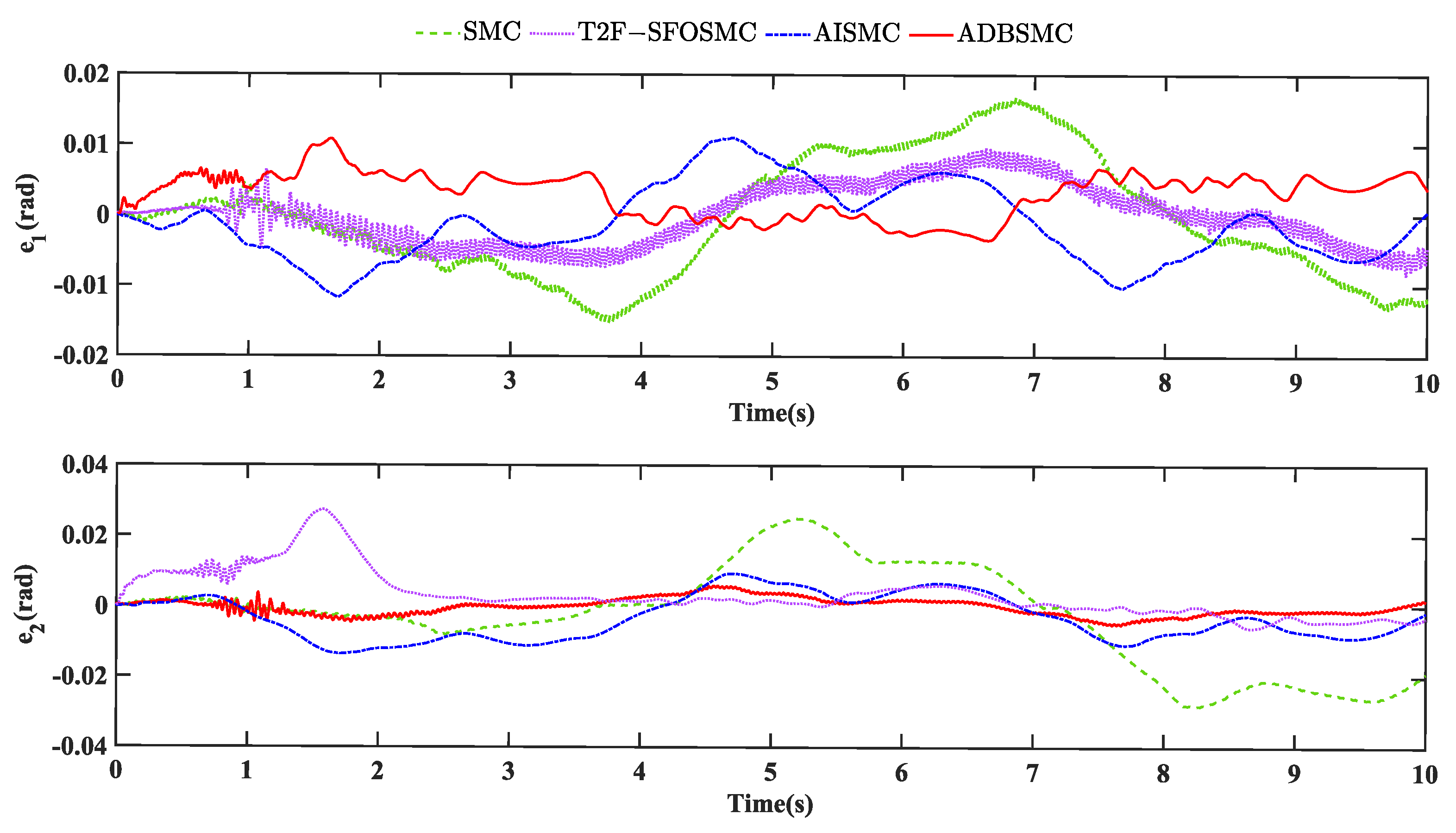
The experimental control parameters were consistent with the simulated control parameters in the previous section. In the mutation disturbance experiments, we also applied an external disturbance of 2 Nm at the joint positions of the robot arm at 3.1 s. The results from the first and second joints of the Franka–Emika–Panda robot were selected for the experimental analysis.

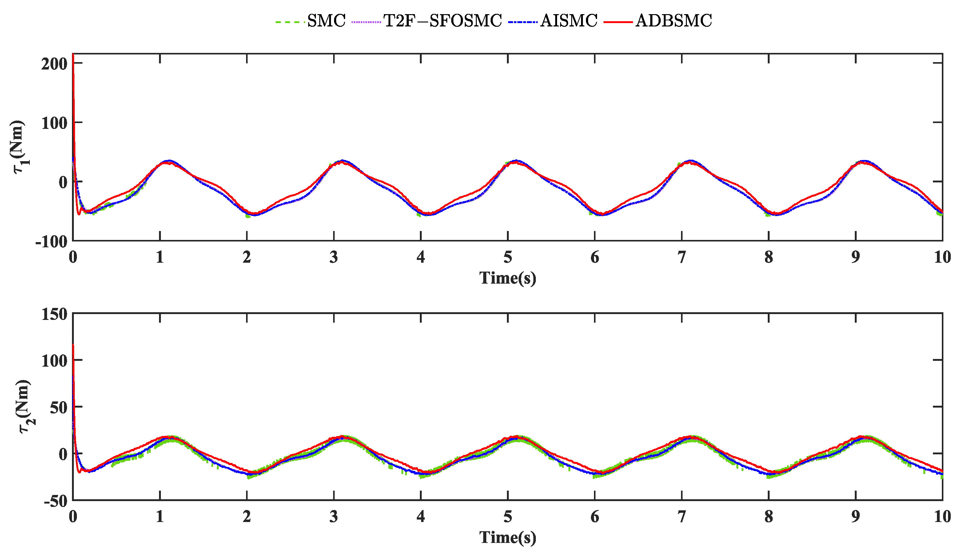
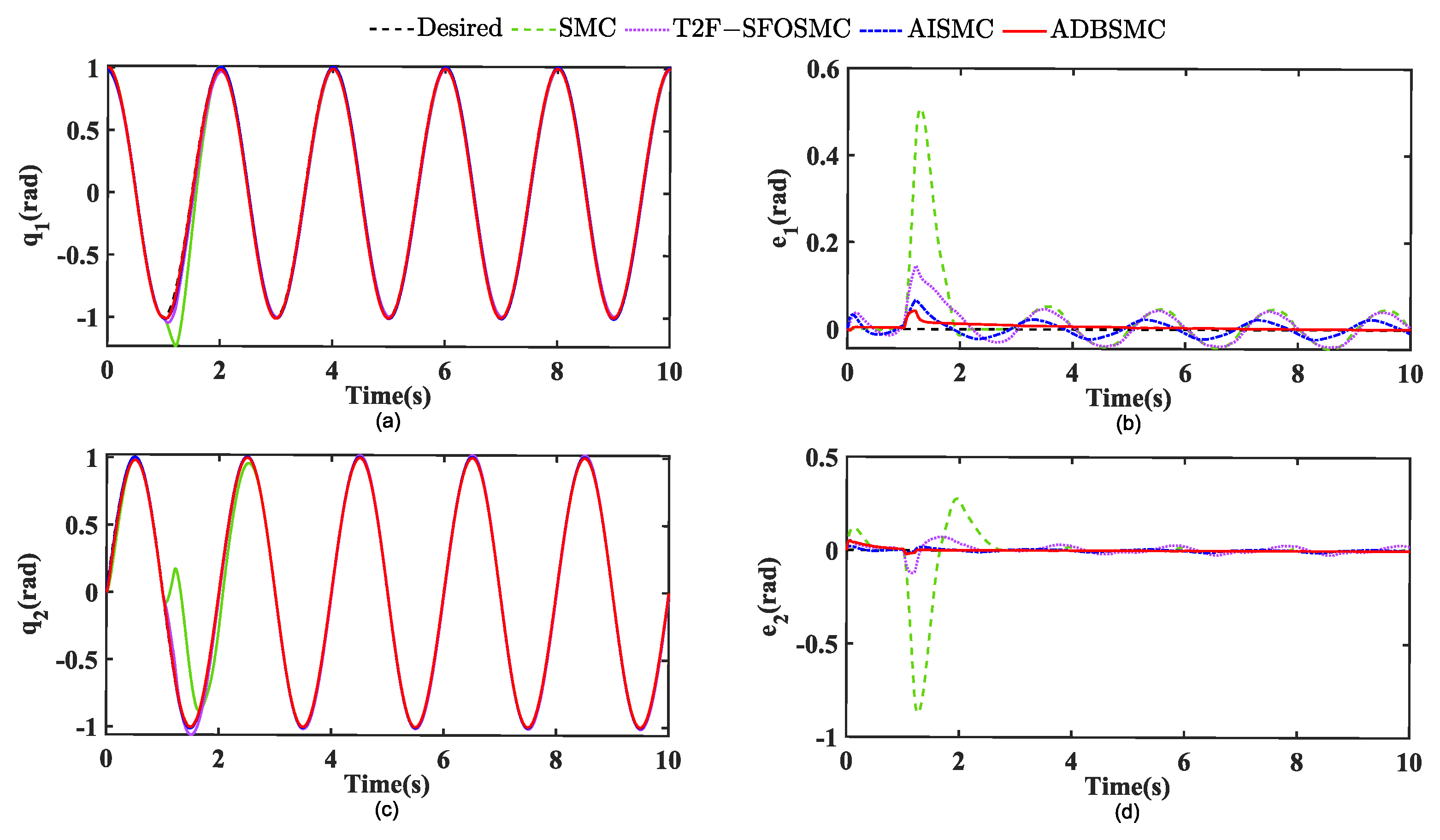
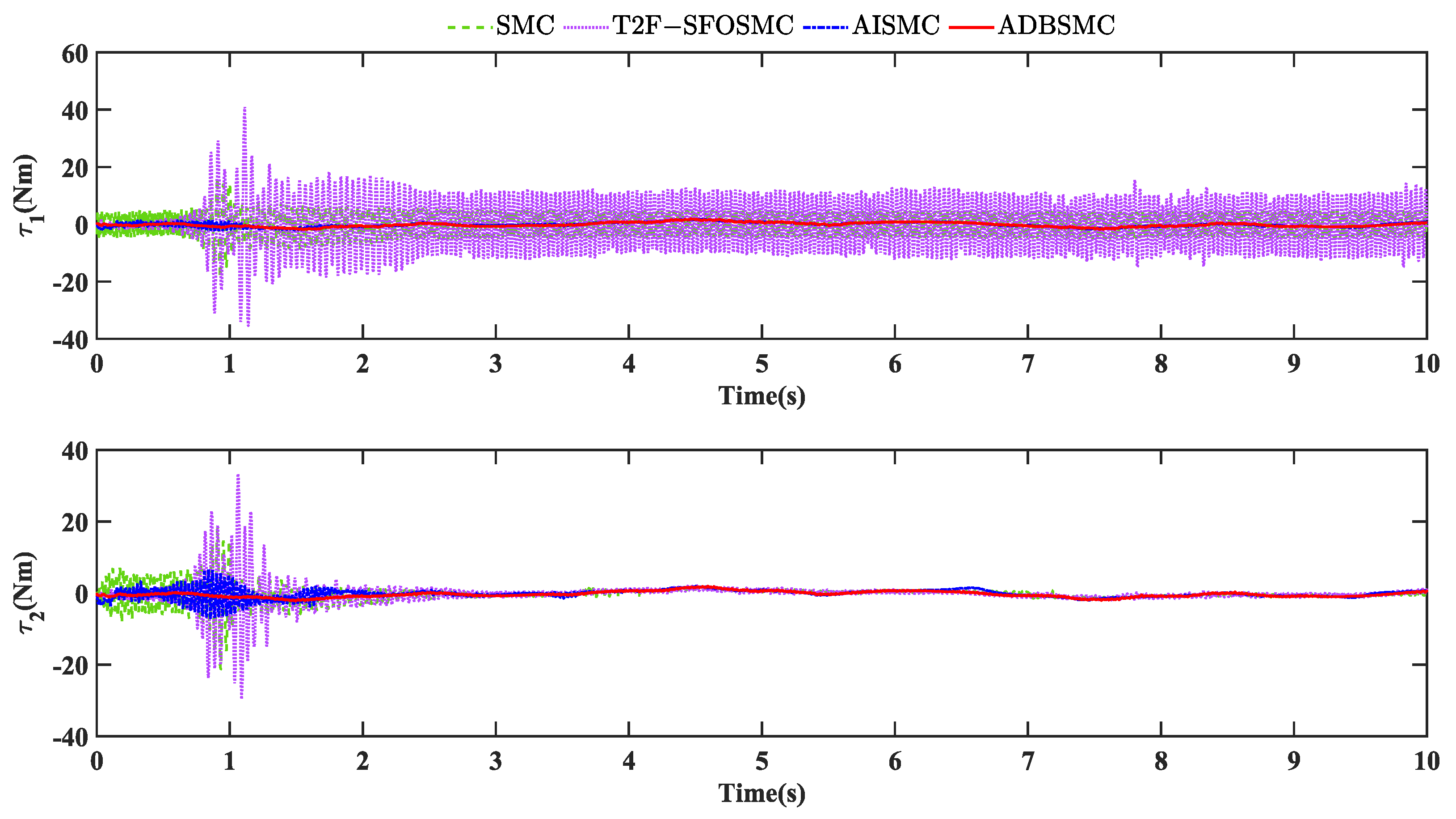
Figure 10 displays that in the presence of disturbances, the error remains minimal for all control methods, with the ADBSMC method exhibiting the most negligible deviation, suggesting its superior disturbance rejection capability. The control input torque, as shown in Figure 11, reveals more about the control strategies’ robustness. While all methods experience initial spikes, indicative of a response to the disturbance, the ADBSMC method demonstrates a more damped torque output over time, pointing to its effectiveness in disturbance compensation and its potential in maintaining system stability under erratic conditions.

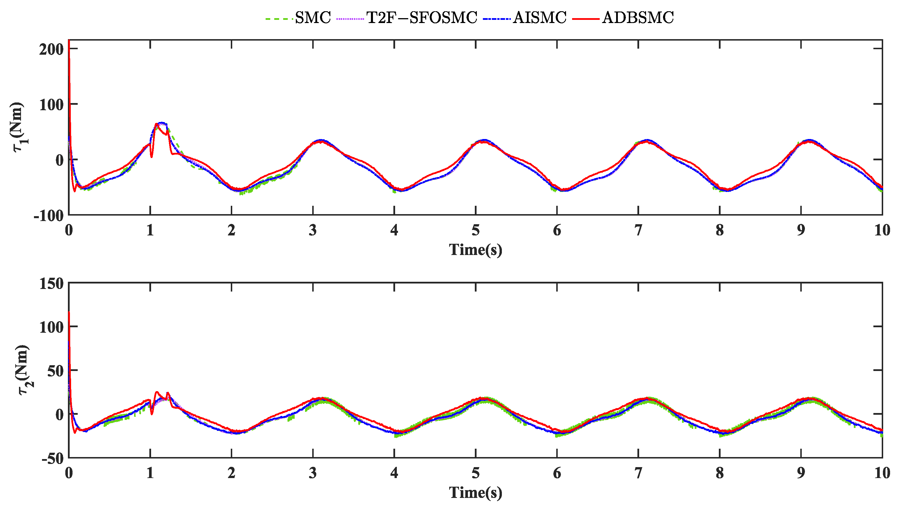
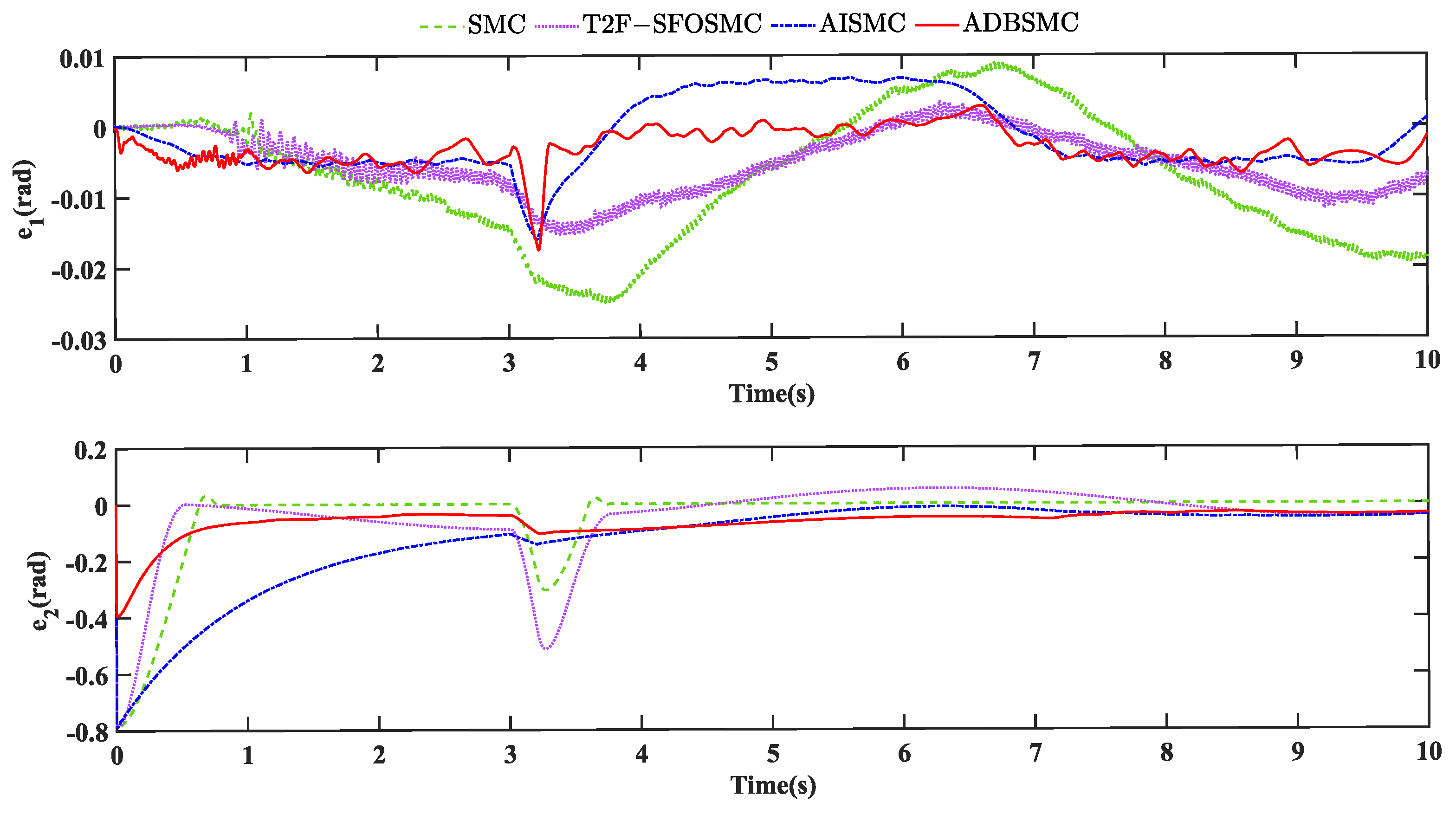
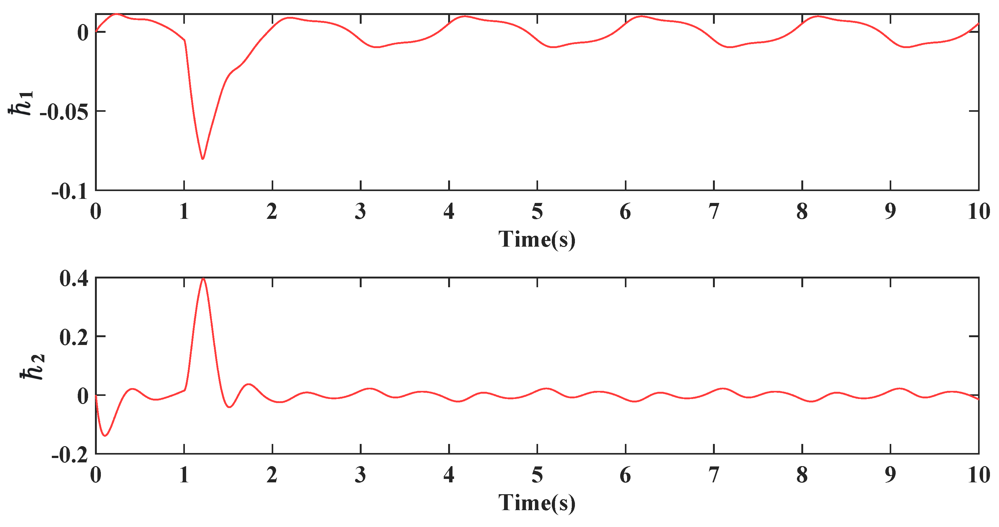
Figure 12 and Figure 13 illustrate the system’s response to a sudden impulse disturbance applied at 3.1 s, represented by a 10 N impact. Figure 12 shows a sharp response to the disturbance, with all control methods rapidly compensating for the error introduced. Notably, the ADBSMC maintains the error within the narrowest bounds, suggesting an effective handling of the abrupt change. Similarly, Figure 13 displays an immediate spike at the moment of impact, reflecting the controllers’ action to counteract the disturbance. The ADBSMC method shows a more composed response post impact, with a smoother return to the baseline torque level, indicating a robust disturbance rejection and a quicker stabilization compared with the other methods. These results underscore the ADBSMC’s potential for high-precision control in dynamic environments, where coping with sudden disturbances is critical for maintaining system performance and stability. Moreover, the margin of error is acceptable.

For better analysis, we calculated the root mean square error (RMSE) and maximum absolute error (MAE) for each case based on the experimental data, which are detailed in

Table 3. Comparison of interference errors under experimental Case One and Case Two.

Controller	Random Disturbance		Impact and Random Disturbance
	Position	Position	Position	Position
	RMSE (rad)	MAE (rad)	RMSE (rad)	MAE (rad)
SMC	0.0274	0.0283	0.0257	0.7652
T2F−SFOSMC	0.0071	0.0274	0.0064	0.8169
AISMC	0.0081	0.0136	0.0102	0.7852
ADBSMC	0.0029	0.0059	0.0007	0.3926

.

Table 3 shows that, as with the simulation results, our proposed controller maintains small RMSE and MAE values even under the influence of external disturbances compared with the SMC, T2F−SFOSMC, and AISMC controllers. This again demonstrates the robustness of our controllers in achieving excellent tracking performance under challenging conditions.

7. Conclusions

The ADBSMC controller proposed in this paper consistently demonstrates effective outcomes, mitigating challenges arising from modeling errors and parameter uncertainties inherent in nonlinear states. The incorporation of an adaptive algorithm enhances control effectiveness, eliminating the necessity for a priori knowledge and encompassing all boundary conditions. For position tracking, the RMSE of the ADBSMC controller is 47.71%, 89.83%, and 47.67% of those from controllers SMC, T2F−SFOSMC, and AISMC, respectively. For MAE, a similar result with RMSE can be obtained. Additionally, the integration of a disturbance observer facilitates both disturbance tracking and compensation. Nevertheless, the robotic arm system itself is complex and susceptible to motor torque saturation. Furthermore, there is always the possibility for online updated estimates of the dynamics of the system by using machine vision. Addressing these challenges may be the focus of future research endeavors to further enhance the overall performance of the proposed control system.

References

1. Xiao, J.; Dou, S.; Zhao, W.; Liu, H. Sensorless human-robot collaborative assembly considering load and friction compensation. IEEE Robot. Autom. Lett. 2021, 6, 5945–5952. [Google Scholar] [CrossRef]
2. Liu, C.; Wen, G.; Zhao, Z.; Sedaghati, R. Neural-network-based sliding-mode control of an uncertain robot using dynamic model approximated switching gain. IEEE Trans. Cybern. 2020, 51, 2339–2346. [Google Scholar] [CrossRef]
3. Schuster, M.; Bernstein, D.; Reck, P.; Hamaza, S.; Beitelschmidt, M. Automated aerial screwing with a fully actuated aerial manipulator. In Proceedings of the 2022 IEEE/RSJ International Conference on Intelligent Robots and Systems (IROS), Kyoto, Japan, 23–27 October 2022; pp. 3340–3347. [Google Scholar]
4. Razmjooei, H.; Shafiei, M.H.; Palli, G.; Arefi, M.M. Non-linear finite-time tracking control of uncertain robotic manipulators using time-varying disturbance observer-based sliding mode method. J. Intell. Robot. Syst. 2022, 104, 36. [Google Scholar] [CrossRef]
5. İlgen, S.; Durdu, A.; Gülbahçe, E.; Çakan, A.; Kalyoncu, M. The bees algorithm approach to determining smc controller parameters for the position control of a scara robot manipulator. Avrupa Bilim Teknol. Derg. 2022, 33, 267–273. [Google Scholar] [CrossRef]
6. Chotikunnan, P.; Chotikunnan, R. Dual design pid controller for robotic manipulator application. J. Robot. Control. 2023, 4, 23–34. [Google Scholar] [CrossRef]
7. Elsisi, M.; Mahmoud, K.; Lehtonen, M.; Darwish, M.M. Effective nonlinear model predictive control scheme tuned by improved nn for robotic manipulators. IEEE Access 2021, 9, 64278–64290. [Google Scholar] [CrossRef]
8. Chotikunnan, R.; Roongprasert, K.; Chotikunnan, P.; Imura, P.; Sangworasil, M.; Srisiriwat, A. Robotic Arm Design and Control Using MATLAB/Simulink. Int. J. Membr. Sci. Technol. 2023, 10, 2448–2459. [Google Scholar]
9. Ilgen, S.; Durdu, A.; Gülbahçe, E.; Çakan, A.; Kalyoncu, M. Optimal tuning of the smc parameters for a two two-link manipulator co-simulation control. Elektron. Elektrotechnika 2021, 27, 4–10. [Google Scholar] [CrossRef]
10. Ahmed, M.S.; Mary, A.H.; Jasim, H.H. Model and chattering free adaptive fuzzy smc for robotic manipulator systems. Tex. J. Eng. Technol. 2022, 8, 33–43. [Google Scholar]
11. Ji, P.; Li, C.; Ma, F. Sliding mode control of manipulator based on improved reaching law and sliding surface. Mathematics 2022, 10, 1935. [Google Scholar] [CrossRef]
12. Fei, J.; Ding, H. Adaptive sliding mode control of dynamic system using RBF neural network. Nonlinear Dyn. 2012, 10, 1563–1573. [Google Scholar] [CrossRef]
13. Carron, A.; Arcari, E.; Wermelinger, M.; Hewing, L.; Hutter, M.; Zeilinger, M.N. Data-driven model predictive control for trajectory tracking with a robotic arm. IEEE Robot. Autom. Lett. 2019, 4, 3758–3765. [Google Scholar] [CrossRef]
14. Xi, R.D.; Xiao, X.; Ma, T.N.; Yang, Z.X. Adaptive sliding mode disturbance observer based robust control for robot manipulators towards assembly assistance. IEEE Robot. Autom. Lett. 2022, 7, 6139–6146. [Google Scholar] [CrossRef]
15. Negrete-Chávez, D.Y.; Moreno, J.A. Second-order sliding mode output feedback controller with adaptation. Int. J. Adapt. Control. Signal Process. 2016, 30, 1523–1543. [Google Scholar] [CrossRef]
16. Edwards, C.; Shtessel, Y.B. Adaptive continuous higher order sliding mode control. Automatica 2016, 65, 183–190. [Google Scholar] [CrossRef]
17. Zhao, H.; Tao, B.; Ma, R.; Chen, B. Manipulator trajectory tracking based on adaptive sliding mode control. Concurr. Comput. Pract. Exp. 2022, 34, e7051. [Google Scholar] [CrossRef]
18. Zaare, S.; Soltanpour, M.R. Adaptive incremental sliding mode control for a robot manipulator. Mech. Syst. Signal Process. 2022, 163, 108165. [Google Scholar] [CrossRef]
19. Han, S.H.; Tran, M.S.; Tran, D.T. Adaptive sliding mode control for a robotic manipulator with unknown friction and unknown control direction. Appl. Sci. 2021, 11, 3919. [Google Scholar] [CrossRef]
20. Jerbi, H.; Al-Darraji, I.; Tsaramirsis, G.; Ladhar, L.; Omri, M. Hamilton–Jacobi Inequality Adaptive Robust Learning Tracking Controller of Wearable Robotic Knee System. Mathematics 2023, 11, 1351. [Google Scholar] [CrossRef]
21. Yin, F.; Wen, C.; Ji, Q.; Zhang, H.; Shao, H. A compensation sliding mode control for machining robotic manipulators based on nonlinear disturbance observer. Trans. Inst. Meas. Control. 2022, 44, 2336–2349. [Google Scholar] [CrossRef]
22. Shi, R.; Zhang, X.; Zhu, Z. A novel fixed-time sliding mode control for nonlinear manipulator systems based on adaptive disturbance observer. Asian J. Control. 2023, 25, 3144–3159. [Google Scholar] [CrossRef]
23. Xian, J.; Shen, L.; Chen, J.; Feng, W. Continuous sliding mode control of robotic manipulators based on time-varying disturbance estimation and compensation. IEEE Access 2022, 10, 43473–43480. [Google Scholar] [CrossRef]
24. Alshammari, O.; Kchaou, M.; Jerbi, H.; Ben Aoun, S.; Leiva, V. A fuzzy design for a sliding mode observer-based control scheme of Takagi-Sugeno Markov jump systems under imperfect premise matching with bio-economic and industrial applications. Mathematics 2022, 10, 3309. [Google Scholar] [CrossRef]
25. Kchaou, M.; Jerbi, H. Reliable H and passive fuzzy observer-based sliding mode control for nonlinear descriptor systems subject to actuator failure. Int. J. Fuzzy Syst. 2022, 24, 105–120. [Google Scholar] [CrossRef]
26. Sachan, S.; Swarnkar, P. Intelligent fractional order sliding mode based control for surgical robot manipulator. Electronics 2023, 12, 729. [Google Scholar] [CrossRef]
27. Wang, Y.; Zhang, Z.; Li, C.; Buss, M. Adaptive incremental sliding mode control for a robot manipulator. Mechatronics 2022, 82, 102717. [Google Scholar] [CrossRef]
28. Petrič, T.; Žlajpah, L. Kinematic model calibration of a collaborative redundant robot using a closed kinematic chain. Sci. Rep. 2023, 13, 17804. [Google Scholar] [CrossRef] [PubMed]
Figure 1. Schematic diagram of the proposed ADBSMC.
Electronics 13 00900 g001
Figure 2. Model of two-degrees-of-freedom manipulator.
Electronics 13 00900 g002
Figure 3. (a) Joint 1 trajectory tracking results; (b) Joint 1 tracking error results; (c) Joint 2 trajectory tracking results; (d) Joint 2 tracking error results.
Electronics 13 00900 g003
Figure 4. Control inputs results under SMC, T2F−SFOSMC, AISMC, and our proposed method.
Electronics 13 00900 g004
Figure 5. Autotuning parameter ( t ) of our proposed ADBSMC.
Electronics 13 00900 g005
Figure 6. (a) Joint 1 trajectory tracking results; (b) Joint 1 tracking error results; (c) Joint 2 trajectory tracking results; (d) Joint 2 tracking error results.
Electronics 13 00900 g006
Figure 7. Control inputs results under SMC, T2F−SFOSMC, AISMC, and our proposed method.
Electronics 13 00900 g007
Figure 8. Case Two: Autotuning parameter ( t ) of our proposed ADBSMC.
Electronics 13 00900 g008
Figure 9. Franka–Emika–Panda robot.
Electronics 13 00900 g009
Figure 10. Tracking error result under random disturbance.
Electronics 13 00900 g010
Figure 11. Control inputs results under random disturbance.
Electronics 13 00900 g011
Figure 12. Tracking error result under impact and random disturbance.
Electronics 13 00900 g012
Figure 13. Control inputs results under impact and random disturbance.
Electronics 13 00900 g013