Abstract
Deep Joint transmitter-receiver optimized communication system (Deep JTROCS) is a new physical layer communication system. It integrates the functions of various signal processing blocks into deep neural networks in the transmitter and receiver. Therefore, Deep JTROCS can approach the optimal state at the system level by the joint training of these neural networks. However, due to the non-differentiable feature of the channel, the back-propagation of Deep JTROCS training gradients is hindered which hinders the training of the neural networks in the transmitter. Although researchers have proposed methods to train transmitters using auxiliary tools such as channel models or feedback links, these tools are not available in many real-world communication scenarios, limiting the application of Deep JTROCS. In this paper, we propose a new method to use undertrained Deep JTROCS to transmit the training signals and use these signals to reconstruct the training gradient of the neural networks in the transmitter, thus avoiding the use of an additional reliable link. The experimental results show that the proposed method outperforms the additional link-based approach in different tasks and channels. In addition, experiments conducted on real wireless channels validate the practical feasibility of the method.
1. Introduction
Artificial intelligence (AI) is widely acknowledged as a pivotal technology for future 6G, with the potential to significantly impact the performance of wireless communication systems. This will further leverage the performance capabilities of communication systems to meet the requirements of future 6G applications, encompassing high reliability, high speed, low latency, and extensive connectivity.
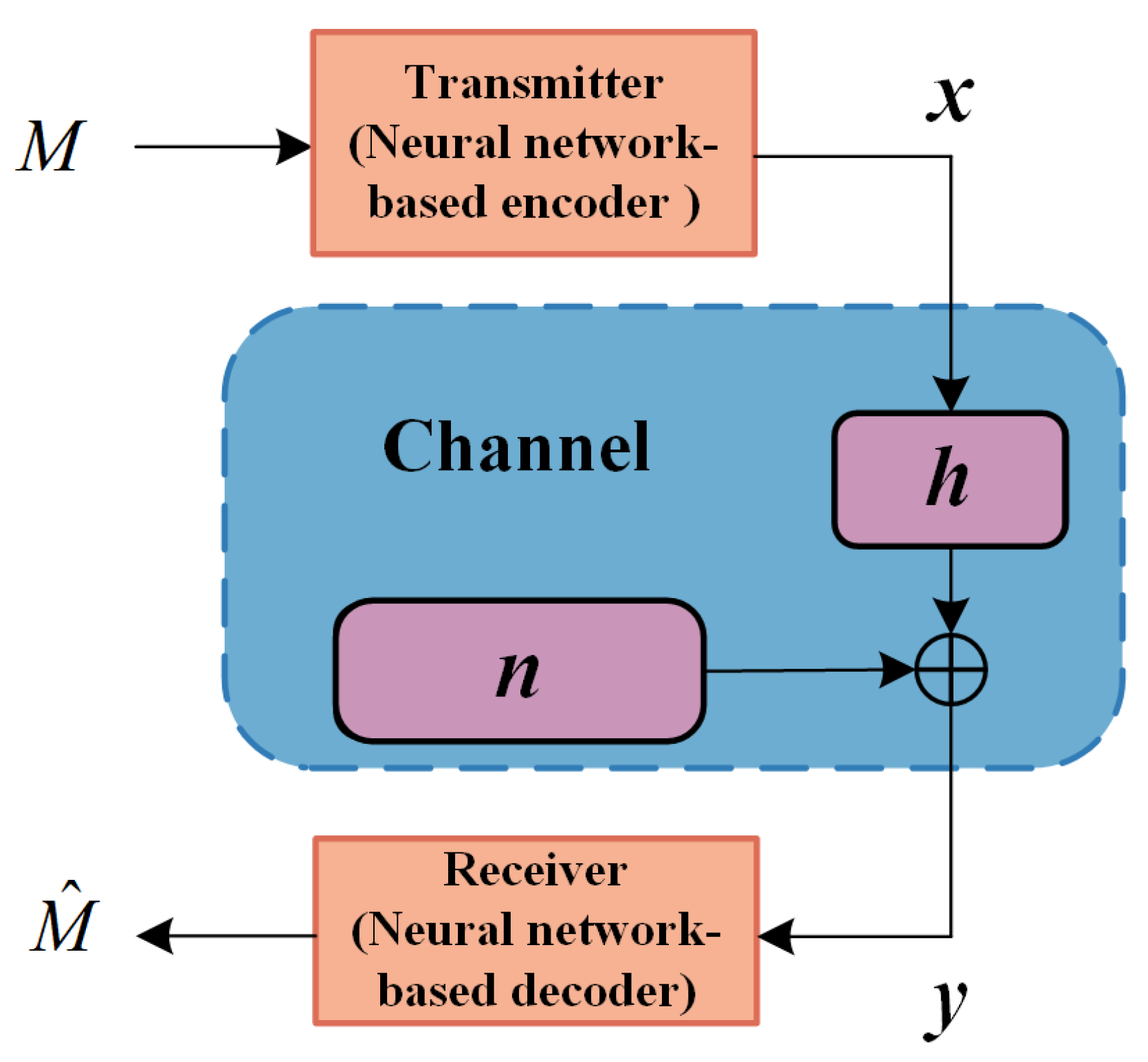
As a promising solution for combining AI with communication systems, the Deep Joint Transmitter-Receiver Optimized Communication System (Deep JTROCS) reshapes the structure of wireless communication systems at the physical layer. In Deep JTROCS, some or all of the digital signal processing functional modules in the transmitter and receiver, such as source coding, channel coding, modulation, source decoding, channel decoding and demodulation, etc., are integrated into a channel-spanning autoencoder consisting of deep neural networks, as shown in Figure 1, where the neural networks in the transmitter and the receiver are referred to as the encoder and decoder, respectively. During training, the encoder and decoder located at the two ends of the system’s working channel collaborate with each other to sense the channel and jointly adjust their parameters based on the channel state so that the communication system achieves better performance on its operating channel.

Figure 1.
The Deep Joint Transmitter-Receiver Optimized Communication System (Deep JTROCS).
Deep JTROCS flexibly adapts to different communication scenarios and gains performance improvements, such as semantic communication [1], orthogonal frequency division multiplexing (OFDM) [2], multiple input multiple output (MIMO) [3,4,5], non-orthogonal multiple access (NOMA) [6], constellation shaping [7] and fiber optic communication systems [8].
However, how to train Deep JTROCS is a difficult problem. The channel and some hardware device components, such as the antenna and the RF front-end, are non-differentiable, which block the back-propagation of the training gradients from the decoder to the encoder. Consequently, the encoder cannot be updated during training due to the unavailability of the gradients.
In some of the existing research, it is common to train Deep JTROCS using differentiable channel models instead of real channels to evaluate the performance of Deep JTROCS on different tasks. Ref. [9] adds a noise vector to the input data of the receiver to simulate the channel interference to the modulation signal, which establishes a complete end-to-end trainable communication system model. However, the channel model is so simple that it ignores the more complex impact of the channel on signals. Refs. [10,11] propose to insert the non-trainable but differentiable additive white Gaussian noise (AWGN) layer between the receiver and transmitter as a channel model. The additional layer has adjustable parameters related to noise variance, which makes the description of the ratio of energy per bit to noise power spectral density more accurate. This model reliably describes the effect of the AWGN channel on signal, but it is not suitable for other types of channels. Ref. [12] follows the conventional idea [13] which views the channel model as a time-varying linear system with additive noise. They use a neural network layer and an additive noise layer to implement the channel model. After the training, the channel model simulates different types of channels. In addition, the conditional generative adversarial networks (CGAN) [14] have been used to simulate different channel effects in [15,16]. Ref. [17] also proposes a residual-assisted GAN (RA-GAN) based training scheme for mitigating gradient vanishing and overfitting in GANs. In addition, Ref. [16] constructs an interesting method for transceiver systems that inserts a CGAN between the transmitter and receiver of each user or base station to simulate the channel. The method causes both transmitters and receivers to converge in training, which allows this system to achieve better results in channels where the uplink and downlink are similar. However, in most real-world low-signal-to-noise communication scenarios, the uplink and downlink have large differences so the method is only applicable to certain scenarios.
Using the channel model to train Deep JTROCS offers a major advantage: The training gradient that passes through the model provides enough information for the encoder in the transmitter to obtain complete channel state information (CSI). This allows the encoder to tune itself based on the entire CSI, resulting in improved performance. Nevertheless, building a channel model for a real channel is a daunting task. Modeling a communication channel in practice is challenging, as it involves transmitting and collecting massive signals from both ends of the real-world channel. If the collected signals lack sufficient channel change states, it may result in neural network over-fitting, leading to the poor performance of Deep JTROCS on real working channels. The acquisition of these signals and the construction of channel models necessitate substantial financial and human resources, leading to a diminished interest among technology developers in integrating Deep JTROCS into actual communication systems. Therefore, Deep JTROCS training based on channel models is not an ideal solution.
To solve the above problem, researchers also propose some approaches that directly train Deep JTROCS without a channel model. Ref. [18] proposes a reinforcement learning-based approach to train encoders in Deep JTROCS. Ref. [19] investigates a gradient-free training method based on a cubic Kalman filter to perform geometric constellation shaping. Ref. [20] proposes two solutions, signal reduction and signal prediction, and verifies the feasibility of both solutions in practical wireless communication systems with super-exotropic architectures, band-pass channel noise and quantization noise. Ref. [21] proposes the use of random perturbation techniques to train deep learning-based communication systems in real channels without assuming channel models. Ref. [22] eliminates the limitation of joint training through meta-learning. In this method, online gradient meta-learning of the decoder is combined with joint training of the encoder through pilot transmission and the use of feedback links. Ref. [23] utilizes a neural estimator of mutual information that relies only on channel samples to optimize the encoder for maximizing mutual information.
Although the above methods allow Deep JTROCS to be trained on real channels, the encoder in the Deep JTROCS transmitter must be updated with the necessary training information available in the receiver, such as the decoder’s loss function or the receiver’s received signals. The training information must be feedback to the transmitter via an additional and reliable low-error communication link. Hence, the practical utility of Deep JTROCS is constrained by the dependence on a low error feedback link. If a conventional communication system is used to provide training information as the feedback link, the question would arise as to why Deep JTROCS, which is complex to train, should be used if the conventional system works appropriately. In addition, untrained Deep JTROCS is not suitable for use as feedback links in these methods due to its large transmission errors.
In this paper, we propose a new training method to solve the above problem. Its main feature is that it can employ untrained and unreliable Deep JTROCS to transmit training signals and employ these signals to reconstruct the training gradient of the encoder. The update of the Deep JTROCS encoder thus is independent of the training information of the receiver, making it feasible to train the transmitter without requiring a feedback link.
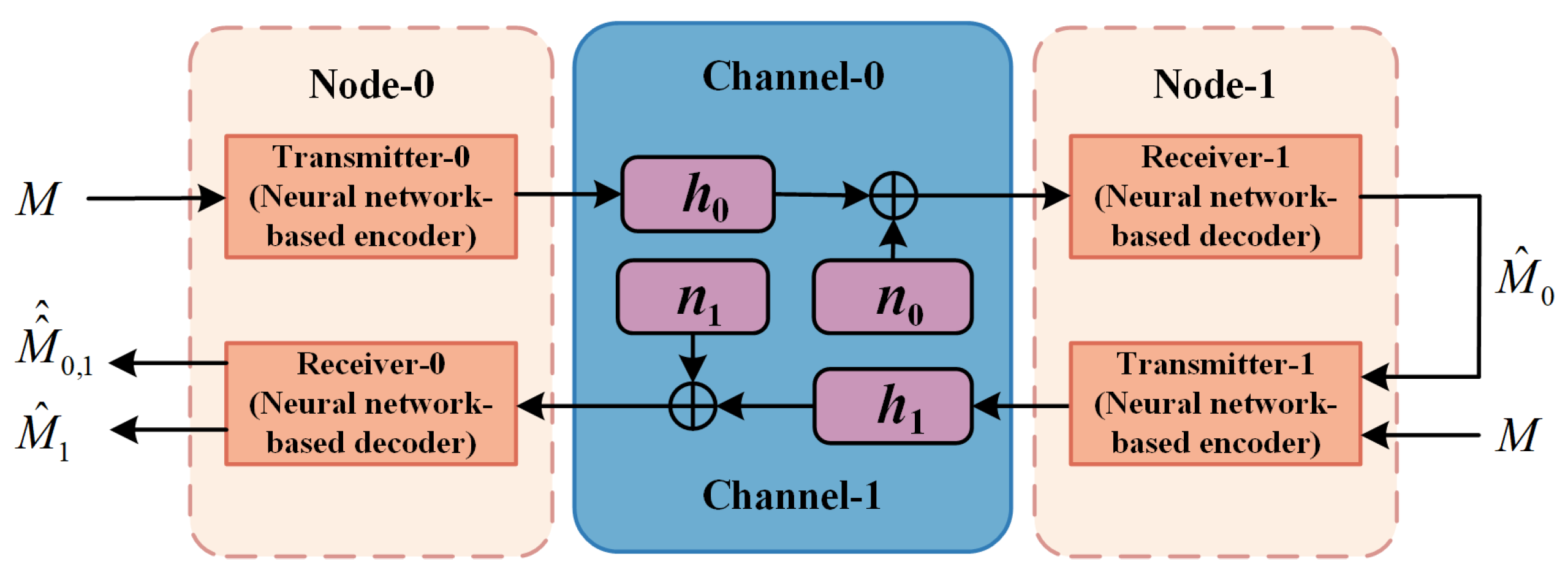
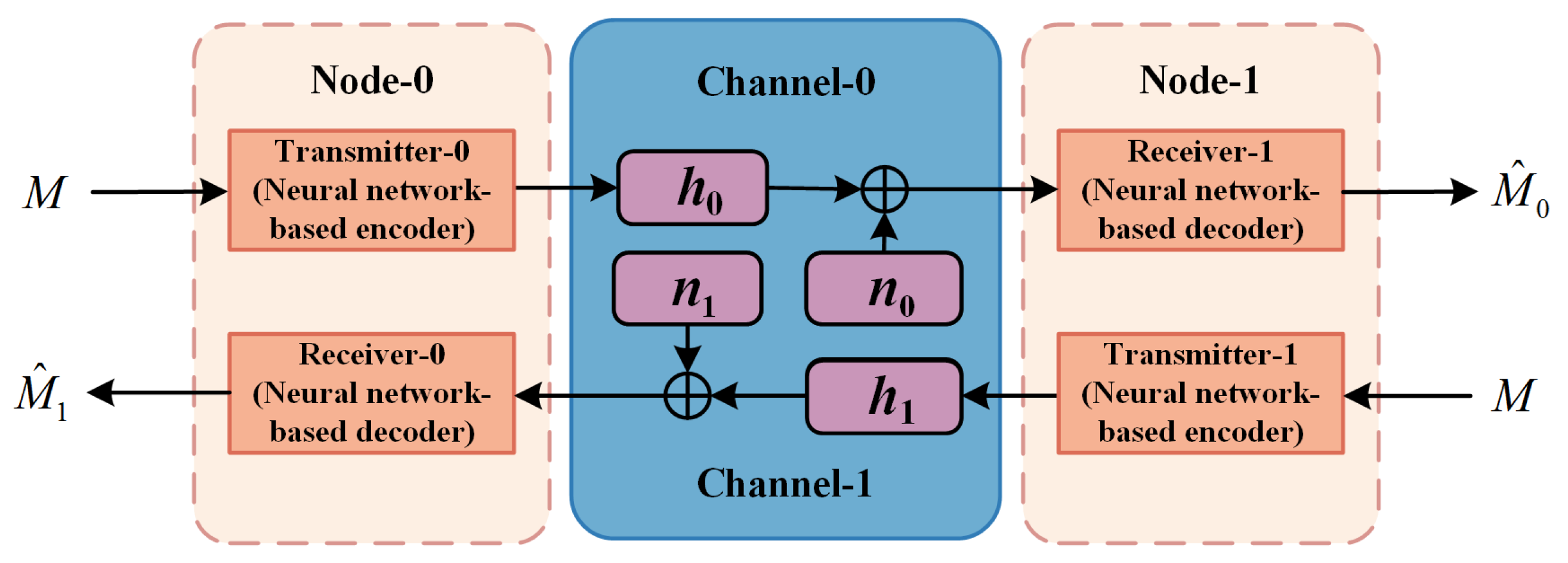
Specifically, we first combine two Deep JTROCS into a dual-node intelligence communication system (DNICS), as shown in Figure 2, where each node has a neural network-based transmitter and receiver. Then, the nodes send training signals to each other and forward the received training signals. Finally, these direct and forwarded training signals are used to estimate the channel state and to reconstruct the training gradients of the transmitters in the nodes.
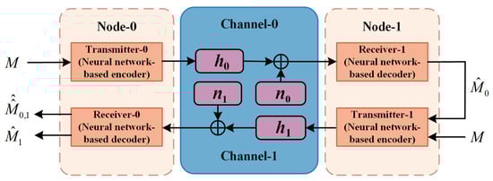
Figure 2.
The dual-node intelligence communication system (DNICS) consisting of two Deep JTROCS.
The proposed training method can effectively train DNICS without the need for auxiliary tools such as channel models or reliable feedback links. This allows for the training of two communication nodes to adapt to the communication environment without the reliance on channel models or training information from the receiver, irrespective of their location, distance, or the complexity of the communication environment.
Additionally, we also implement real-time online training of a DNICS on a real-world channel in the experiment, which indicates that the proposed method has solved the training problem of Deep JTROCS. Deep JTROCS, therefore, has the basis to be applied in real communication scenarios.
The main contributions of our work are summarized as follows:
- We propose a new Deep JTROCS training approach, which combines two Deep JTROCS into a DNICS and allows the unreliable Deep JTROCS to transmit and forward training signals to evaluate the channel state and reconstruct the training gradient of the transmitter.
- The experimental results show that the proposed method can work with different types of sources and channels. When the difference between uplink and downlink is large, the proposed method can still work well.
- We implement a DNICS, which can be trained online in real-time without any auxiliary tools, on a real-world channel.
2. Problem Description
The transmitting signal M of Deep JTROCS is a number or sequence that comes from a discrete set , which is encoded by the Deep JTROCS transmitter,
where f, and x denote the neural network-based encoder in the transmitter, the encoder parameters and the encoder output, respectively.
x then is sent into the channel,
where h and are two stochastic variables that denote the channel response and additive noise, respectively. Note, that the channel described in (2) is a broad definition that also includes the physical devices that interfere with the training of the neural network, such as antennas and RF-front ends, etc.
y is a damaged version of x, the Deep JTROCS receiver uses it to rebuild the source signal,
where the , g and represent the reconstruction signal, the neural network-based decoder in the receiver and the decoder parameters, respectively.
In a reliable communication system, the reconstructed signal must be sufficiently similar to M. We, therefore, need to adjust the parameters of the neural network in the transmitter and receiver to minimize the impact of the channel on Deep JTROCS in training.
where is the loss function of the receiver which describes the overall system error.
However, the real channel is non-differentiable and the neural network in the transmitter does not have the training gradient available. The system can be trained by (4) when only the channel model is used in place of the real channel. Therefore, only the decoder in the receiver is trained by the supervised learning directly, as shown in (5).
To train the transmitter on the real channels, an efficient idea is to use the loss function of the decoder to reconstruct the gradient of the encoder, which makes the transmitter know the error of the whole system; Ref. [18] gives a feasible and specific way to implement this, as shown in (6),
where S, and are the batch size, the loss function of the receiver and the gradient of the output of the encoder after relaxation (26), respectively.
Nevertheless, this approach is not available in many real-world scenarios because it requires an additional reliable link to transmit from the receiver to the transmitter, but such a low-error reliable link does not exist in many scenarios.
3. The Proposed Training Approach
An effective way to avoid the use of additional communication links in the encoder training is to find an alternative function that is available at the transmitter side to replace the in (6).
The common communication system usually consists of multiple user nodes that contain both transmitters and receivers, and signals are transmitted and forwarded between these nodes. We can use these transmitted and forwarded signals to find the alternative function of . Therefore, we build the DNICS based on Deep JTROCS to analyze the transmission and forwarding of the signals in the node-based communication system.
3.1. The Dual-Node Intelligence Communication System Model
The DNICS, as shown in Figure 2, is a minimal model of the node-based communication system that describes the system with only two nodes. In DNICS, the transmitter and the receiver from different Deep JTROCS are constituted to be a node, which represents a single user or a network with multiple users.
The signals in DNICS can be transmitted between Node-0 and Node-1 to each other. According to (1)–(3), the direct reconstruction signals and in Figure 3 can be described as
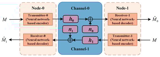
Figure 3.
The signal transmission in DNICS.
For a practical communication system, the reconstructed signals should be as similar as possible to the source signals, and the similarity is described by the loss functions (9) and (10). The smaller the loss function, the more stable the communication system.
The loss is calculated from the cross entropy (CE) (11) of the digital signals or the mean square error (MSE) (12) of the analog signals, respectively.
where k, p and N denote the sample point index of z and , the probability distributions, and the length of the samples.
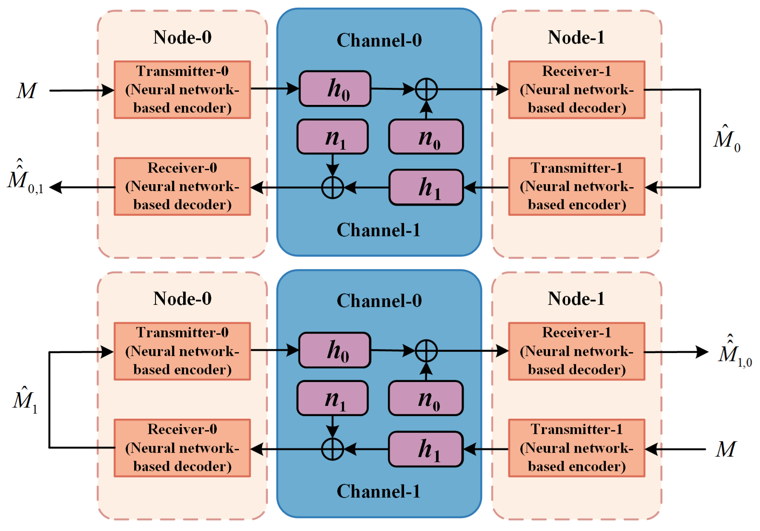
In DNICS, and are also forwarded back to their source nodes and are reconstructed as and , as shown in Figure 4.
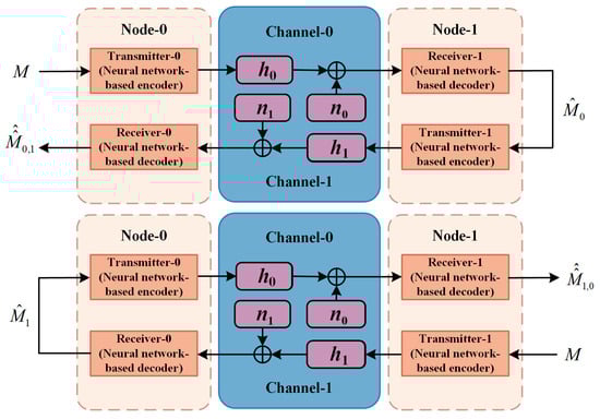
Figure 4.
The signal forwarding in DNICS.
Obviously, we can use these signals transmitted and forwarded in DNICS to find the desired alternative function.
3.2. The Alternative Function
Assuming that the channel is relatively stable, i.e., the changes in the distributions of and are not significant, and the encoder g and decoder f do not correct their parameters and during transmission of the signal, will be constantly approaching , when is approaching M.
where → indicates that the vector to its left is constantly approaching the vector to its right. (17) is also written as
The condition in (18) is negligible because the training of Deep JTROCS is the process it describes.
Therefore, is a desirable function that is used in place of the loss function to avoid transmitting the decoder loss function of Node-1, because both and are available at Node-0, as shown in Figure 2. Similarly, the encoder in Node-1 is trained by .
is an ideal function as the loss function for training the encoder in Transmitter-i. It effectively characterizes an approximation of the error of Deep JTROCS on Channel-i, with the difference between this approximation and the actual error attributed to the varying states of Channel-j () at different times. Computing using and is equivalent to channel estimation for Channel-i, implicitly providing partial channel state information for Transmitter-i when the acquisition times of and are very close (i.e., when the channel state does not change significantly).
3.3. Training of Encoders in DNICS
According to [18], the training gradient of the encoder in Node-i is obtained by finding the partial derivative of the variable with respect to the loss function (21).
where , and are the expectation, the loss value of decoder in Node-j and the stochastic channel, respectively. (22) is also rewritten as (23).
where is the Dirac distribution approximated by the Gauss distribution with a very small standard deviation .
where and are the mean and standard deviation, respectively.
According to (19) and (20), we use and , which are available at Node-i, to train the encoder in Node-i, as shown in (27). The specific training procedure of the encoders is given in Algorithm 1.
| Algorithm 1 The training algorithm of encoders. |
|
3.4. Training of DNICS
The encoders and decoders in DNICS are trained alternately, as shown in Algorithm 2, where Transmitter-i and Receivers-i denote the transmitter and receiver in the Node-i, respectively. Note, that the encoder is updated first and the decoder then follows their change.
| Algorithm 2 The alternating training algorithm. |
|
The decoders are directly trained by supervised learning (5). The specific training process of the receiver is given in Algorithm 3.
| Algorithm 3 Training algorithm of decoders. |
|
3.5. The Win-Win Phenomenon in the Training of DNICS
We observe an interesting win-win phenomenon in training where the two Deep JTROCS in DNICS help each other to reduce their errors.
When the loss value (10) of the Deep JTROCS link (8) decreases with the updating of the encoder and decoder parameters during the training, the error of (8) and (13) decreases, which favors the reduction in the Node-0 loss value of the encoder in the middle, thus reducing the loss value (9) of the Deep JTROCS link (7).
It allows our approach to complete the training in fewer epochs than [18] and also makes the training easier to converge.
4. Experiments
In this section, the proposed approach is compared with the channel model-based MA [12] and the feedback link-based MF [18] approaches on different tasks, such as the transmission of digital symbols, binary symbol sequences, and analog signals. The performance of these training approaches is evaluated by the performance of the trained Deep JTROCS (or Deep JTROCS in DNICS). The better the performance of the trained communication system, the better the performance of the approach.
The dataset for the transmission of digital symbols and binary symbol sequences consists of randomly generated symbols, while the dataset for the transmission of analog signals consists of randomly intercepted music clip samples. The labels of the samples in these datasets are the samples themselves. Specific details about the datasets are given in the respective experiment subsections.
The different channel states in the experiments are simulated by the channel models. However, only MA uses these channel models directly to back-propagate the gradients, and neither MF nor our approach uses these channel models to transmit the training gradients.
The structures of the encoders and decoders in Deep JTROCS or are different in different tasks, which are given in specific subsections. The neural networks are trained by the Stochastic Gradient Descent (SGD) and Adam [24] optimizers, respectively, and the learning rates are set to . The optimizer selection and setting results are obtained from experiments.
Additionally, this work focuses on the training approach for neural networks in Deep JTROCS. Consequently, we utilize metrics commonly employed to evaluate neural networks, such as accuracy, to describe the performance of training approaches in experiments, rather than traditional communication system metrics like bit error rate.
4.1. Transmission of Digital Symbols
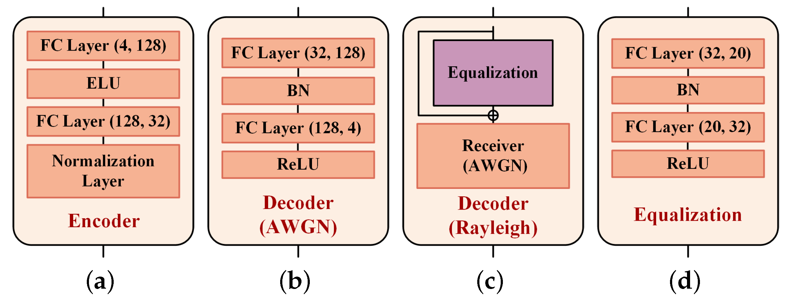
In this experiment, Deep JTROCS is trained to transmit digital symbols on AWGN and Rayleigh channels. The structures of the encoder and decoder are shown in Figure 5. The encoder consists of two fully connected (FC) layers and a normalization layer. The first FC layer has 128 ELU [25] activated neurons, and the other layer has 32 neurons without activation function. The normalization layer limits the output amplitude of the neural network to meet the system limits on output power. For the AWGN channel, the decoder is implemented by two FC layers with batch normalization (BN) [26] and ReLU [27] activation. Their neuron numbers are 128 and 4, respectively. For the Rayleigh channel, the decoder is composed of an additional equalization and the receiver of the AWGN channel. The equalization is used to estimate the channel response. It is a neural network with two FC layers, where the first FC layer has 20 hyperbolic tangent (Tanh) activated neurons, and the other layer has 32 neurons without activation function.
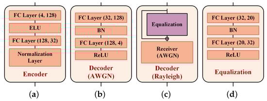
Figure 5.
The neural network structure of transmitter and receiver in transmission of digital symbol. (a) Encoder; (b) Decoder-A; (c) Decoder-R; (d) Equalization.
The experimental dataset consists of a training set, a validation set and a testing set containing 16,384, 8192 and 8192 samples. Each sample in these datasets is a digital symbol represented by a one-hot vector of length 4.
Table 1 and Table 2 show the test accuracy of DNICS and Deep JTROCS on AWGN and Rayleigh simulation channels, respectively. The MA and MF in the tables denote Deep JTROCS trained by the channel model [12] and the reliable feedback link [18], respectively. Ours-0 shows the performances with a different signal-to-noise ratio (SNR) in different channel directions, and one direction of the channel remains 0 dB SNR. Ours-1 denotes the Deep JTROCS performance of DNICS trained on the channels with the same SNR in different directions. The values inside and outside the brackets indicate the accuracy in different directions, respectively.

Table 1.
The accuracy of symbol transmission on Additive white Gaussian noise (AWGN) channels.
Table 2.
The accuracy of symbol transmission on Rayleigh channels.
The results show that DNICS trained by our approach achieves similar accuracy to that of Deep JTROCS trained by MA and MF. As the SNR decreases, the accuracy of the communication system decreases regardless of the training method used. When SNR is small enough, e.g., SNR = −10 dB, the accuracy of MA is better than that of MF and Ours because the channel model provides more complete state information of the simulated experimental channel for training the communication system than other approaches. However, the channel model is not a real channel and it does not provide real CSI for the training of Deep JTROCS; instead, our approach trains two Deep JTROCS directly on their working channel online and in real time.
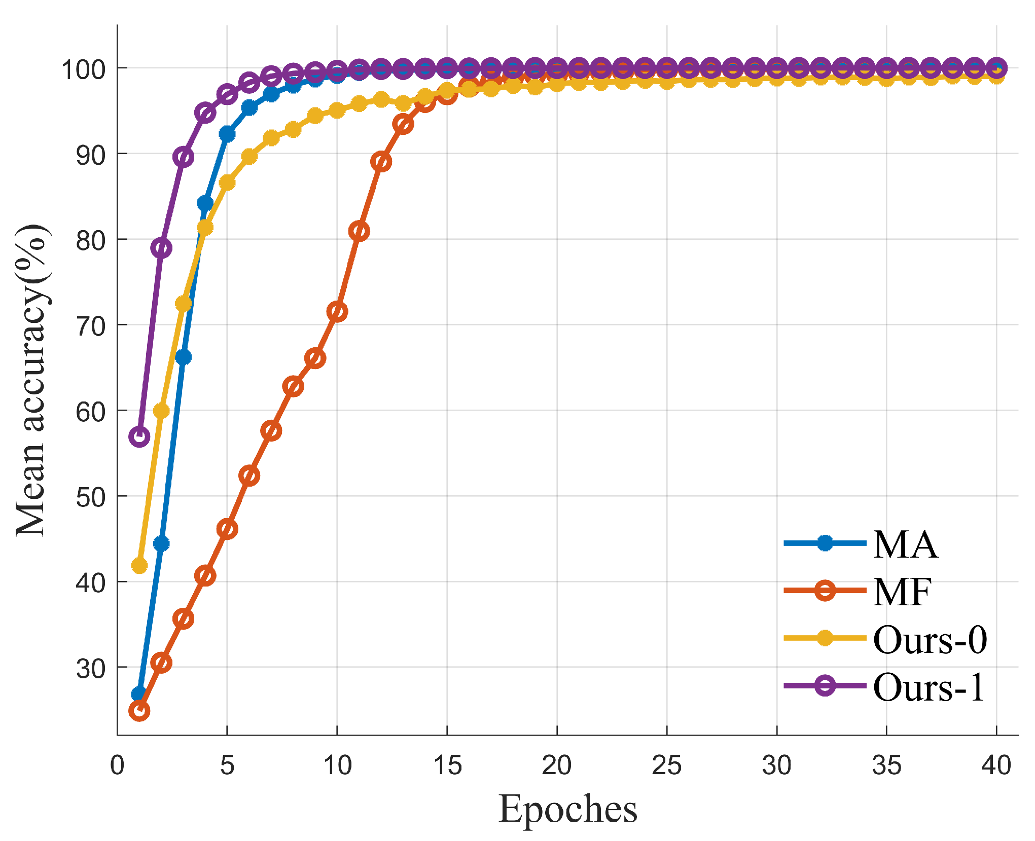
Figure 6 shows the variation in training accuracy of the trained Deep JTROCS over the first 40 training epochs. All these curves are obtained with the same training parameters, where the batch size is 128, the learning rate is and the channel is AWGN. The SNR of the channel is 0 dB in MA and MF, 0 dB (−5 dB) and 0 dB (0 dB) in Ours-0 and Ours-1, where the numbers inside and outside the brackets indicate the SNR in different channel directions, respectively. The accuracy of Ours-0 and Ours-1 is the mean of two Deep JTROCS in two channel directions.

Figure 6.
Accuracy and epoch evolution of training.
Figure 6 indicates that the Deep JTROCS trained by our approach requires fewer training epochs to reach 100% accuracy than Deep JTROCS trained by FM and MA at 0 dB. We believe that the win-win phenomenon in our proposed approach accelerates the convergence of Deep JTROCS in training.
4.2. Transmission of Binary Symbol Sequence
In order to finely observe the performance differences of Deep JTROCS trained by different approaches, we used square waves composed of repeated sample points to represent the binary symbol sequence and used the mean accuracy of the sample points to evaluate the performance of trained system structures. In addition, we added the bandwidth limit of the Deep JTROCS in this experiment to further simulate the real communication environment.
The experimental dataset contains 8192 samples, of which 90% are the training set, 5% are the validation set and 5% are the test set. Each sample contains 512 randomly generated binary symbols, and each symbol is represented by 32 repeated sample points with the values of 1 or 0.
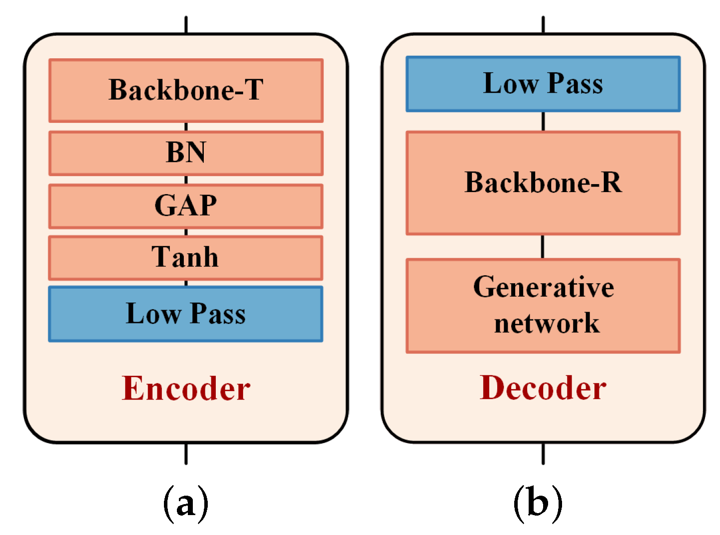
The encoder and decoder are implemented by the 1D convolution neural networks (CNN), as illustrated in Figure 7. The encoder consists of a backbone network, a BN layer, a global average pooling (GAP) layer, a Tanh layer and a low-pass filter. The backbone is the SEResNet-18 [28,29] without the final average pooling layer and full connection layer. It is used to extract the features and encode the input samples. The GAP layer maps the output to the size of , where 8192 denotes the length of network output and 2 indicates that the output signal has the in-phase and the quadrature components. The BN and tanh layers restrict the amplitude of the network output signal. The low-pass filter layer is used to limit the bandwidth of the output signals. The decoder of receivers is designed as an encoder-decoder structure to reduce the noise [30]. It consists of a backbone network (SEResNet-18) and a generative network composed of five fractionally-strided convolution layers with an output GAP layer. The hyperparameters of these fractionally-strided convolution layers are shown in Table 3. In addition, a low-pass filter is placed in front of the decoder to filter some noise out of the working bandwidth.
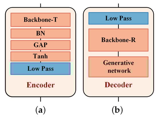
Figure 7.
The structure of encoder and decoder in transmission of binary symbol sequence. (a) Encoder; (b) Decoder.
Table 3.
The hyperparameters of the fractionally-strided convolution layers in the decoder.
Table 4 and Table 5 show the experimental results on AWGN and Rayleigh channels, respectively. Note, that the results in the table are the accuracy per sample-point in the transmitted symbols.
Table 4.
The accuracy of binary symbol sequence transmission on AWGN channels.
Table 5.
The accuracy of binary symbol sequence transmission on Rayleigh channels.
Specifically, the accuracy of Ours-1 is very close to that of MA, while the accuracy of MF and Ours-0 are lower than that of Ours-1 and MA. The system trained by Ours-1 benefits from the channel estimation in the forwarding mechanism and achieves comparable performance to MA. However, when the SNR of two directions is different, the direction of the channel with a smaller SNR generates a larger transmission error, which increases the error of the forwarded signal and reduces the accuracy of Deep JTROCS in the direction of the larger SNR.
4.3. Transmission of Analog Signals
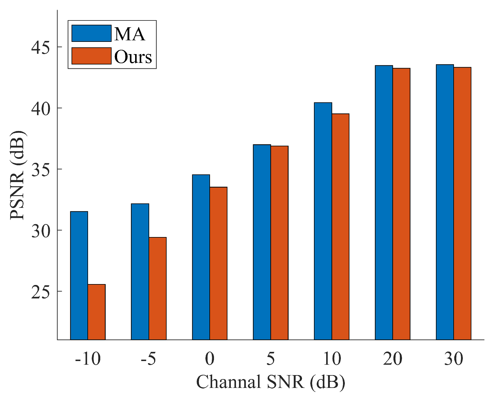
The experiment shows the ability of Deep JTROCS trained with our approach to recover the signal amplitude at different SNRs. The results are shown in Figure 8 and Figure 9, where Deep JTROCS trained by the MA is used as the control group.
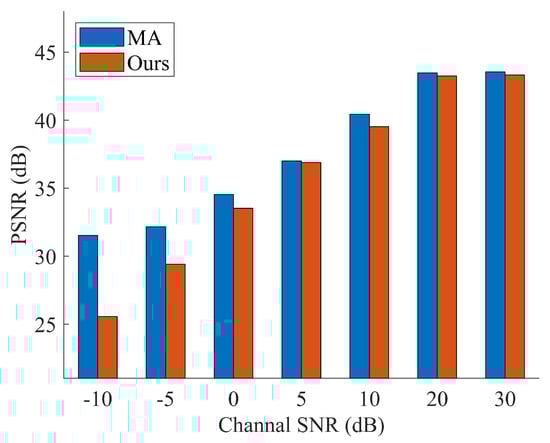
Figure 8.
The Peak Signal-to-noise ratio (PSNR) of reconstructed signals on AWGN channels.
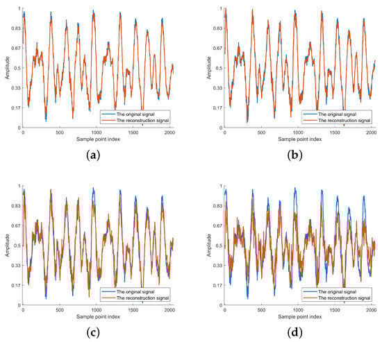
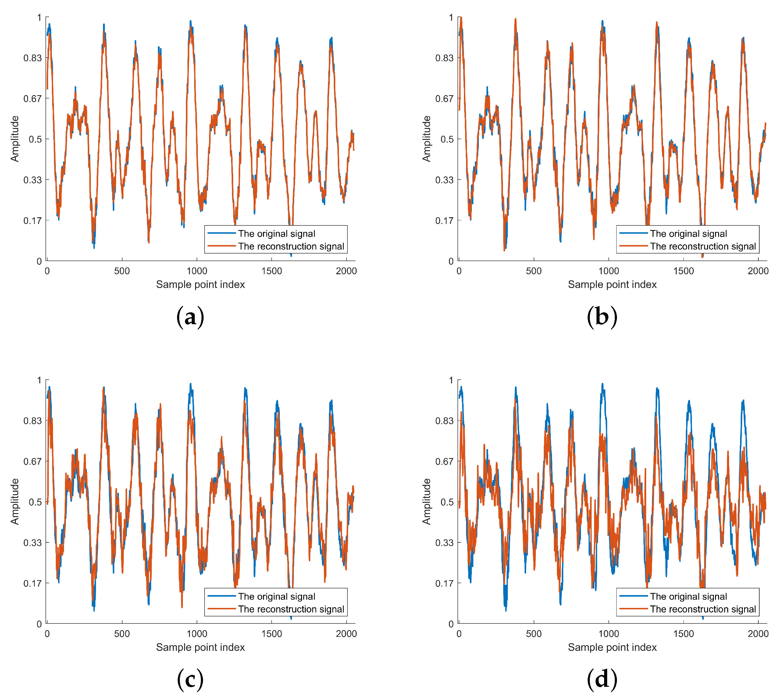
Figure 9.
The reconstructed signal of Deep JTROCS trained by proposed approach. (a) 30 dB; (b) 10 dB; (c) 0 dB; (d) −5 dB.
The experimental signal samples are taken randomly from 11 pieces of music with a sampling rate of 44.1 kHz, and each sample contains 2048 sample points whose values are quantified to a range from 0 to 1 with a minimum quantization interval of ; 90% and 10% samples from the first 8 pieces of music are used for the training and validation, respectively, while the samples from the remaining three pieces of music are used for the test.
The training loss is calculated by the MSE and the quality of the reconstructed signal is evaluated by the PSNR (28),
where z and are normalized to .
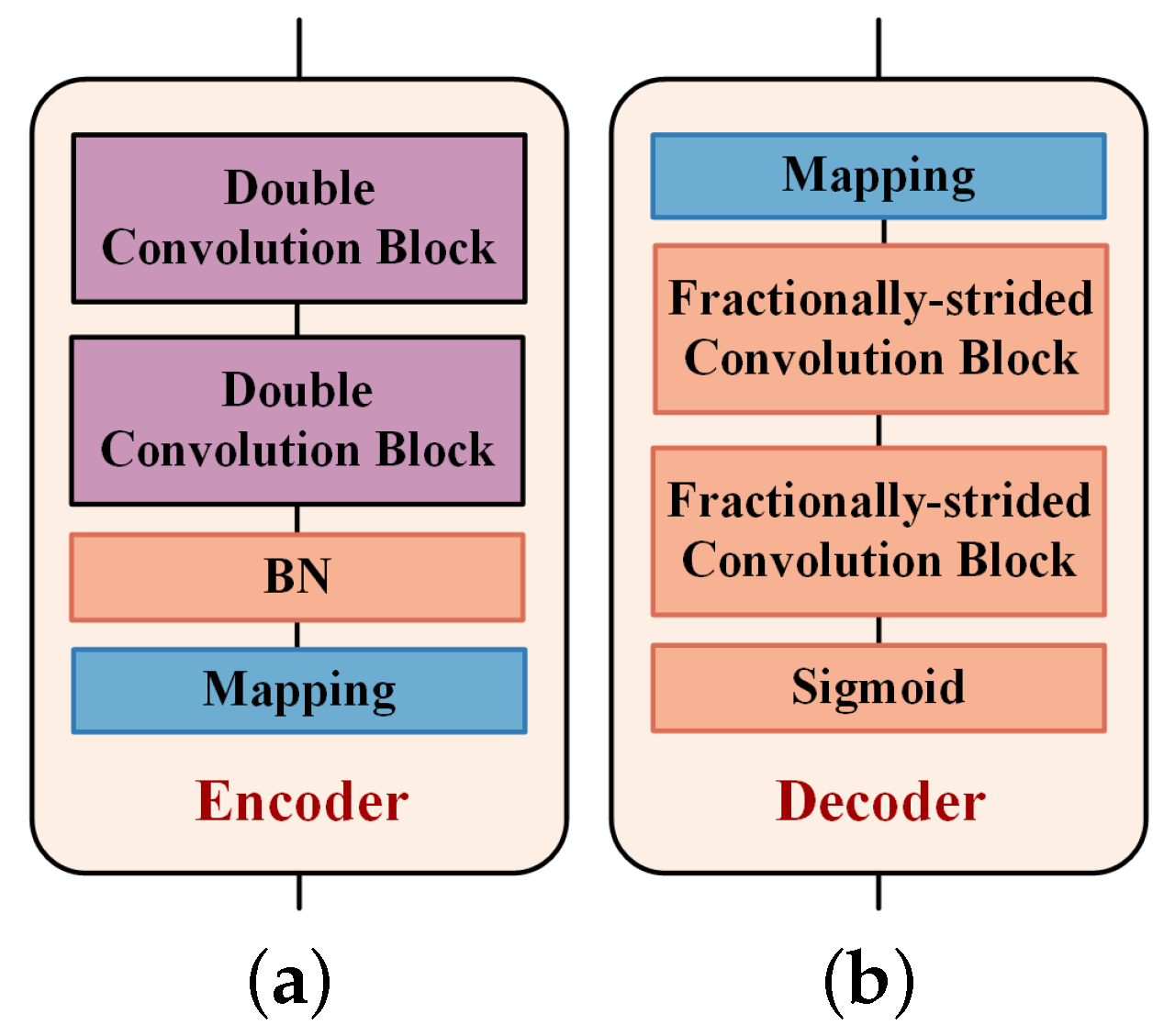
The encoder and decoder are illustrated in Figure 10, where the encoder includes two double convolution blocks, a Sigmoid layer and a mapping function, and the decoder includes a mapping function, two fractionally-strided convolution blocks and a Sigmoid layer. The double convolution block consists of two 1D convolution layers with BN, a ReLU activation layer and a maximum pooling layer. The fractionally-strided convolution block consists of two 1D fractionally-strided convolution layers with a BN and a ReLU activation layer. The mapping function in the transmitter and receiver reshapes the input data to the size of and , respectively.
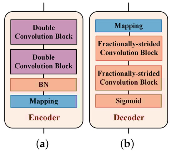
Figure 10.
The neural network structure of transmitter and receiver in symbol sequence experiment. (a) Encoder; (b) Decoder.
Figure 8 shows the comparison between MA and Our-1. Obviously, the performance of the two Deep JTROCS is very similar at high SNR. As the SNR increases, the PSNRs also increase in very close increments. However, at low SNR, the performance of Our-1 is lower than that of MA. This difference in performance is due to the fact that the MA method provides Deep JTROCS with complete channel information, but in real communication environments it is difficult to construct a channel model with complete channel information to train Deep JTROCS.
Figure 9 shows the original signal M and the reconstructed signal of Deep JTROCS trained by our approach at different SNRs. Obviously, the distortion of becomes more and more severe as the SNR decreases. However, the main contours of M are still preserved at low SNRs. This suggests that we can use methods similar to image restoration to repair transmitted signals with high-frequency distortion.
4.4. Summary
The experimental results of the three different tasks indicate that the compared training approaches in the experiment yield similar performance in these tasks. Specifically, the accuracy of MA surpasses that of MF and Ours, owing to the channel model’s capability to furnish comprehensive CSI for the encoders, in contrast to other methodologies. Our approach implicitly estimates the channel state and delivers partial channel state information for Transmitter-i, thereby achieving performance superior to MF and approaching that of MA.
Although all three approaches demonstrate very similar performance, our approach stands out due to its superior practicality. This is attributed to its capability to provide real-time and online training for Deep JTROCS without relying on auxiliary tools, such as channel models and feedback links.
5. Over-the-Air Experiment
To verify the applicability of our approach to real-world channels, we trained DNICS on a composite over-the-air channel. The results are compared with Deep JTROCS trained by MF using a local area network (LAN) as the noise-free feedback link.
5.1. Experimental Setup
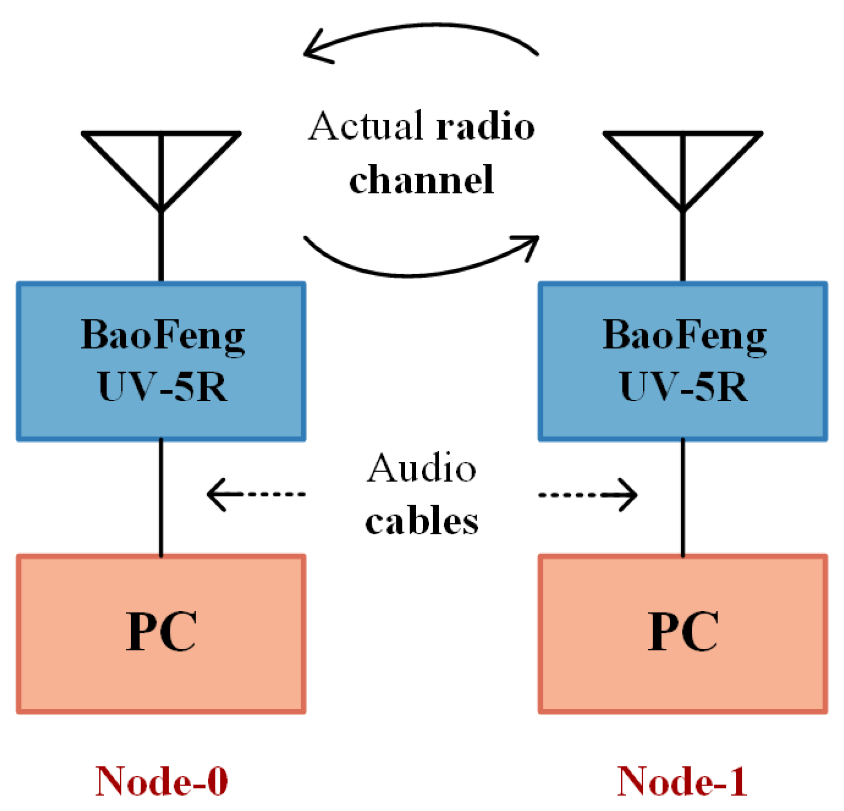
Figure 11 gives an overview of the experimental testbed. The encoders and decoders are located in two personal computers (PCs), and the composite channel consists of two audio cables, two FM intercoms (BaoFeng UV-5R) and a radio channel. The testbed is located in our office of no more than 20 square meters, and the radio channel is an unobstructed line of sight (LOS) of approximately 3 m with multi-path effects. The location of the intercoms remains constant during the training.
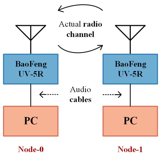
Figure 11.
Testbed overview.
The training task and the neural network structure are consistent with these in Section 4.1, the only difference is the systems transmit binary symbols. The training sample is firstly randomly generated and then distributed to each communication node.
The synchronization of the signals is solved in a two-stage way. In the first stage, a large time window is used to capture the transmitted signal. For example, a signal that lasts 1 s needs to be captured using a window of more than 1 s. In the second stage, the position of each symbol is located by detecting the preambles inserted in signals.
5.2. Result
Figure 12 shows that the variation in accuracy of Deep JTROCS over the first 170 training epochs, where Node-0, Node-1 and MF denote the accuracy variation of two nodes of DNICS trained by our approach and Deep JTROCS trained by MF, respectively. After no more than 150 epochs, the accuracy of both Deep JTROCS are improved to 100%. Additionally, Figure 12 also shows that DNICS requires fewer epochs for convergence than the MF-trained Deep JTROCS, but its growth is unstable. We speculate that this is the result of the win-win effect of our method.
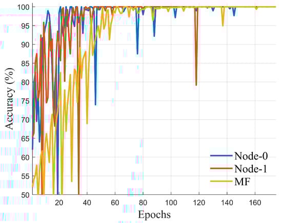
Figure 12.
Evolution of accuracy.
This experiment demonstrates that our method can train Deep JTROCS in real-time online over complex real channels without any auxiliary tools.
6. Conclusions
In this paper, we propose a new training approach for Deep JTROCS that combines two Deep JTROCS into a DNICS and alternately updates the encoders and decoders. Specifically, the encoders are updated by the damage of the transmitted signals in the channel, which is calculated from the forwarding and direct reconstruction signals in the DNICS, and the decoders are trained by supervised learning. Therefore, the proposed approach makes Deep JTROCS more practical as Deep JTROCS can be trained on the real-world channel and without any tools. Furthermore, we experimentally observe that the Deep JTROCS in DNICS reinforce each other in a win-win manner, accelerating the convergence of accuracy during training.
Theoretically, Deep JTROCS senses the channel and achieves optimum communications performance by, for example, adjusting the transmit power and timing of the signal. Although our training approach provides the transmitter with a loss to describe the damage caused by the channel to the transmitted signal, this value does not provide the transmitter with full CSI. Therefore, in the future, we continue to search for system architectures and training approaches that provide full CSI to the transmitter of Deep JTROCS.
Author Contributions
Conceptualization, W.S.; Investigation, Y.H.; Methodology, W.S. and Y.H.; Validation, T.Y., Z.W. and Y.M.; Writing—original draft, W.S.; Writing—review and editing, W.S. and Y.H. All authors have read and agreed to the published version of the manuscript.
Funding
This research was funded by The LongYuan Youth Innovation and Entrepreneurship Talent (Individual) Project grant number 2023LQGR38.
Data Availability Statement
The data presented in this study are available on request from the corresponding author. The data are not publicly available due to the music copyright.
Conflicts of Interest
Author Yuchen He was employed by the company The Silk Road Fantian (Gansu) Communication Technology Co., Ltd. The remaining authors declare that the research was conducted in the absence of any commercial or financial relationships that could be construed as potential conflicts of interest.
References
- Weng, Z.; Qin, Z. Semantic Communication Systems for Speech Transmission. IEEE J. Sel. Areas Commun. 2021, 39, 2434–2444. [Google Scholar] [CrossRef]
- Felix, A.; Cammerer, S.; Dörner, S.; Hoydis, J.; Ten Brink, S. OFDM-Autoencoder for End-to-End Learning of Communications Systems. In Proceedings of the 2018 IEEE 19th International Workshop on Signal Processing Advances in Wireless Communications (SPAWC), Kalamata, Greece, 25–28 June 2018; pp. 1–5. [Google Scholar] [CrossRef]
- Li, J.; Zhang, Q.; Xin, X.; Tao, Y.; Tian, Q.; Tian, F.; Chen, D.; Shen, Y.; Cao, G.; Gao, Z.; et al. Deep Learning-Based Massive MIMO CSI Feedback. In Proceedings of the 2019 18th International Conference on Optical Communications and Networks (ICOCN), Huangshan, China, 5–8 August 2019; pp. 1–3. [Google Scholar] [CrossRef]
- Ji, S.; Li, M. CLNet: Complex Input Lightweight Neural Network Designed for Massive MIMO CSI Feedback. IEEE Wirel. Commun. Lett. 2021, 10, 2318–2322. [Google Scholar] [CrossRef]
- Guo, J.; Wen, C.K.; Jin, S. Deep Learning-Based CSI Feedback for Beamforming in Single- and Multi-Cell Massive MIMO Systems. IEEE J. Sel. Areas Commun. 2021, 39, 1872–1884. [Google Scholar] [CrossRef]
- Ye, N.; Li, X.; Yu, H.; Zhao, L.; Liu, W.; Hou, X. DeepNOMA: A Unified Framework for NOMA Using Deep Multi-Task Learning. IEEE Trans. Wirel. Commun. 2020, 19, 2208–2225. [Google Scholar] [CrossRef]
- Aoudia, F.A.; Hoydis, J. Joint Learning of Probabilistic and Geometric Shaping for Coded Modulation Systems. In Proceedings of the GLOBECOM 2020—2020 IEEE Global Communications Conference, Taipei, Taiwan, 7–11 December 2020; pp. 1–6. [Google Scholar] [CrossRef]
- Li, M.; Wang, D.; Cui, Q.; Zhang, Z.; Deng, L.; Zhang, M. End-to-end Learning for Optical Fiber Communication with Data-driven Channel Model. In Proceedings of the 2020 Opto-Electronics and Communications Conference (OECC), Taipei, Taiwan, 4–8 October 2020; pp. 1–3. [Google Scholar] [CrossRef]
- Varasteh, M.; Piovano, E.; Clerckx, B. A Learning Approach to Wireless Information and Power Transfer Signal and System Design. In Proceedings of the ICASSP 2019—2019 IEEE International Conference on Acoustics, Speech and Signal Processing (ICASSP), Brighton, UK, 12–17 May 2019; IEEE: Piscataway, NJ, USA. [Google Scholar] [CrossRef]
- O’Shea, T.; Hoydis, J. An Introduction to Deep Learning for the Physical Layer. IEEE Trans. Cogn. Commun. Netw. 2017, 3, 563–575. [Google Scholar] [CrossRef]
- Morocho-Cayamcela, M.E.; Njoku, J.N.; Park, J.; Lim, W. Learning to Communicate with Autoencoders: Rethinking Wireless Systems with Deep Learning. In Proceedings of the 2020 International Conference on Artificial Intelligence in Information and Communication (ICAIIC), Fukuoka, Japan, 19–21 February 2020; IEEE: Piscataway, NJ, USA, 2020. [Google Scholar] [CrossRef]
- Ye, H.; Li, G.Y.; Juang, B.H.F. Deep Learning based End-to-End Wireless Communication Systems without Pilots. IEEE Trans. Cogn. Commun. Netw. 2021, 7, 702–714. [Google Scholar] [CrossRef]
- Rappaport, T.S. Wireless Communications: Principles and Practice; Prentice Hall PTR: Upper Saddle River, NJ, USA, 1996; Volume 2. [Google Scholar]
- Mirza, M.; Osindero, S. Conditional Generative Adversarial Nets. arXiv 2014, arXiv:1411.1784. [Google Scholar]
- Ye, H.; Li, G.Y.; Juang, B.H.F.; Sivanesan, K. Channel Agnostic End-to-End Learning Based Communication Systems with Conditional GAN. In Proceedings of the 2018 IEEE Globecom Workshops (GC Wkshps), Abu Dhabi, United Arab Emirates, 9–13 December 2018; IEEE: Piscataway, NJ, USA, 2018. [Google Scholar] [CrossRef]
- Baek, S.; Moon, J.; Park, J.; Song, C.; Lee, I. Real-Time Machine Learning Methods for Two-Way End-to-End Wireless Communication Systems. IEEE Internet Things J. 2022, 9, 22983–22992. [Google Scholar] [CrossRef]
- Jiang, H.; Dai, L. End-to-End Learning of Communication System without Known Channel. In Proceedings of the ICC 2021—IEEE International Conference on Communications, Online, 14–23 June 2021; pp. 1–5. [Google Scholar] [CrossRef]
- Aoudia, F.A.; Hoydis, J. Model-Free Training of End-to-End Communication Systems. IEEE J. Sel. Areas Commun. 2019, 37, 2503–2516. [Google Scholar] [CrossRef]
- Jovanovic, O.; Yankov, M.P.; Da Ros, F.; Zibar, D. Gradient-Free Training of Autoencoders for Non-Differentiable Communication Channels. J. Light. Technol. 2021, 39, 6381–6391. [Google Scholar] [CrossRef]
- Chen, Z. Signal Restoration and Prediction for End-to-End Learning of Practical Wireless Communication System. In Proceedings of the 2022 IEEE 19th International Conference on Mobile Ad Hoc and Smart Systems (MASS), Denver, Colorado, 20–22 October 2022; pp. 654–660. [Google Scholar] [CrossRef]
- Raj, V.; Kalyani, S. Backpropagating through the Air: Deep Learning at Physical Layer without Channel Models. IEEE Commun. Lett. 2018, 22, 2278–2281. [Google Scholar] [CrossRef]
- Park, S.; Simeone, O.; Kang, J. End-to-End Fast Training of Communication Links without a Channel Model via Online Meta-Learning. In Proceedings of the 2020 IEEE 21st International Workshop on Signal Processing Advances in Wireless Communications (SPAWC), Atlanta, GA, USA, 26–29 May 2020; pp. 1–5. [Google Scholar] [CrossRef]
- Fritschek, R.; Schaefer, R.F.; Wunder, G. Deep Learning for Channel Coding via Neural Mutual Information Estimation. In Proceedings of the 2019 IEEE 20th International Workshop on Signal Processing Advances in Wireless Communications (SPAWC), Cannes, France, 2–5 July 2019; pp. 1–5. [Google Scholar] [CrossRef]
- Kingma, D.P.; Ba, J. Adam: A Method for Stochastic Optimization. arXiv 2014, arXiv:1412.6980. [Google Scholar]
- Clevert, D.A.; Unterthiner, T.; Hochreiter, S. Fast and Accurate Deep Network Learning by Exponential Linear Units (ELUs). arXiv 2015, arXiv:1511.07289. [Google Scholar]
- Ioffe, S.; Szegedy, C. Batch Normalization: Accelerating Deep Network Training by Reducing Internal Covariate Shift. arXiv 2015, arXiv:1502.03167. [Google Scholar]
- Glorot, X.; Bordes, A.; Bengio, Y. Deep Sparse Rectifier Neural Networks. In Proceedings of the 14th International Conference on Artificial Intelligence and Statisitics (AISTATS) 2011, Fort Lauderdale, FL, USA, 11–13 April 2011; Volume 15, pp. 315–323. [Google Scholar]
- He, K.; Zhang, X.; Ren, S.; Sun, J. Deep Residual Learning for Image Recognition. arXiv 2015, arXiv:1512.03385. [Google Scholar]
- Hu, J.; Shen, L.; Albanie, S.; Sun, G.; Wu, E. Squeeze-and-Excitation Networks. arXiv 2017, arXiv:1709.01507. [Google Scholar]
- Hinton, G.E.; Salakhutdinov, R.R. Reducing the Dimensionality of Data with Neural Networks. Science 2006, 313, 504–507. [Google Scholar] [CrossRef] [PubMed]

Disclaimer/Publisher’s Note: The statements, opinions and data contained in all publications are solely those of the individual author(s) and contributor(s) and not of MDPI and/or the editor(s). MDPI and/or the editor(s) disclaim responsibility for any injury to people or property resulting from any ideas, methods, instructions or products referred to in the content. |
© 2024 by the authors. Licensee MDPI, Basel, Switzerland. This article is an open access article distributed under the terms and conditions of the Creative Commons Attribution (CC BY) license (https://creativecommons.org/licenses/by/4.0/).