Cognitive Enhancement of Robot Path Planning and Environmental Perception Based on Gmapping Algorithm Optimization

Abstract

In the logistics warehouse environment, the autonomous navigation and environment perception of the logistics sorting robot are two key challenges. To deal with the complex obstacles and cargo layout in a warehouse, this study focuses on improving the robot perception and navigation system to achieve efficient path planning and safe motion control. For this purpose, a scheme based on an improved Gmapping algorithm is proposed to construct a high-precision map inside a warehouse through the efficient scanning and processing of environmental data by robots. While the improved algorithm effectively integrates sensor data with robot position information to realize the real-time modeling and analysis of warehouse environments. Consequently, the precise mapping results provide a reliable navigation basis for the robot, enabling it to make intelligent path planning and obstacle avoidance decisions in unknown or dynamic environments. The experimental results show that the robot using the improved Gmapping algorithm has high accuracy and robustness in identifying obstacles and an effectively reduced navigation error, thus improving the intelligence level and efficiency of logistics operations. The improved algorithm significantly enhances obstacle detection rates, increasing them by 4.05%. Simultaneously, it successfully reduces map size accuracy errors by 1.4% and angle accuracy errors by 0.5%. Additionally, the accuracy of the robot’s travel distance improves by 2.4%, and the mapping time is reduced by nine seconds. Significant progress has been made in achieving high-precision environmental perception and intelligent navigation, providing reliable technical support and solutions for autonomous operations in logistics warehouses.

1. Introduction

With the rapid evolution of e-commerce and supply chain management, warehousing and logistics sorting as an important field has become increasingly prominent [1]. In the complex network of the supply chain, the role of logistics sorting is crucial [2], which includes the classification, distribution, and packaging of various types of goods according to the order or destination [3]. In large warehouses and sorting centers, efficient and accurate sorting operations are critical to reducing logistics costs, improving customer service levels, and strengthening market competitiveness. To achieve efficient logistics sorting, automation technology and sorting robots are widely used in the field of logistics warehousing [4]. Automated sorting systems can significantly improve sorting speed and accuracy [5], thereby reducing labor costs and sorting error rates [6]. However, in the process of automatic sorting, the robot must have the ability to identify and avoid various obstacles to ensure safe and efficient operation [7].

The core tasks of the logistics sorting robot are to realize autonomous navigation in a dynamic and complex storage environment and to have the ability for obstacle recognition and collision avoidance. At present, many researchers are focusing on research and development in the field of logistics sorting robots and have proposed a variety of excellent design schemes and implementation strategies. Chen Yun [8] established a warehouse shelf model, introduced the Poisson distribution to simulate the influence of unknown factors; and established a three-color grid map, which can safely and effectively design the optimal path in the storage environment under the influence of unknown factors and solve the problem of blind search and deadlock. Aiming to solve the multi-automatic guided vehicle (multi-AGV) path problem in logistics and warehousing, a non-dominated sorting differential evolution (NSDE) algorithm was advocated by Duan and Liu [9] to minimize the number of AGVs and the maximum pickup time. It can adjust the picking points in the area, optimize the picking path, and improve the picking efficiency. Wu et al. [10] put forward an FAGV hybrid dynamic path planning algorithm based on improved A* and improved DWA. The improved A* algorithm can plan a globally optimal path that is more suitable for FAGV. The improved DWA evaluation function can ensure that the local path of FAGV is closer to the global path, and the algorithm can dynamically avoid obstacles without being far from the globally optimal path. Yuan Xianfeng and Dong Lin et al. [11] introduced an improved grey wolf optimization algorithm (IGWO) to improve the shortcomings of grey wolf optimization (GWO) in avoiding the premature local optimum and falling into the local optimum. The improved algorithm can plan a shorter and safer path. To improve the accuracy of the ant colony algorithm to find the path and reduce the number of turns, Chen Tao et al. recommended a jump point search-improved ant colony optimization hybrid algorithm. The initial pheromone concentration distribution obtained by the jump point is introduced to guide the algorithm to find the path, which accelerates the early iteration speed of the algorithm. It shows good performance in path finding accuracy and reducing the number of turns [12]. Yang Dong, Wu Yaohua, and Huo Dengya [13] advocated for an effective method to evaluate the picking efficiency and time of the system under the single instruction operation cycle by analyzing the cross-channel shuttle access system. The objective function of the minimum total cost of the system is constructed under the condition of satisfying the customer’s demand, which can lead to the design of a more reasonable storage system under the minimum cost control. Zhang Honglin et al. [14] simultaneously optimized the key issues in automated warehouses, namely, task scheduling (TS) and multi-agent path discovery (MAPF). They put forward a task scheduling algorithm based on enhanced HEFT, a heuristic MAPF algorithm, and a TS-MAPF algorithm to solve this combinatorial optimization problem. These new algorithms perform well. Achirei and Stefan Daniel et al. [15] proposed an object detector to better understand the robot environment and newly acquired datasets. The model is optimized to run on a mobile platform installed on the robot. A model-based predictive controller is introduced. Based on the target map obtained by a customized training CNN detector and lidar data, the omnidirectional robot is guided to a specific position in the logistics environment. Target detection helps the omnidirectional mobile robot obtain a safe, optimized, and efficient path.

The purpose of this paper is to study and explore a method to improve the Gmapping algorithm and the performance of logistics sorting robots in storage environments, especially in autonomous navigation and obstacle recognition. As a probabilistic SLAM algorithm, the Gmapping algorithm is of great significance to constructing maps and locating robots in unknown environments in real time and has been successfully applied in many fields [16]. This study combines laser sensor data and visual odometry to establish a high-resolution grid map to describe the warehouse environment more accurately. The enhanced algorithm initiates environmental scanning preprocessing using a laser rangefinder, obtaining highly accurate three-dimensional data of the surroundings. Subsequently, this laser rangefinder data is fused with visual odometry from a monocular camera. The improved Gmapping algorithm, thus refined, amalgamates information from the laser rangefinder and visual odometry to achieve a more precise mapping of the logistics warehouse environment. In practical implementation, the laser rangefinder contributes high-precision distance information, facilitating the construction of a detailed environmental map. Simultaneously, visual odometry from the monocular camera tracks the camera’s motion, providing crucial position and orientation data. The fusion of these two sensor modalities optimizes the Gmapping algorithm, tailoring it to mapping tasks within the logistics warehouse setting and achieving a high-precision map of the warehouse environment.

The ultimate goal is to realize the accurate mapping of the logistics warehouse environment, serving as a reliable foundation for subsequent autonomous navigation and path planning. This improved Gmapping algorithm, which integrates laser rangefinder and visual odometry data, enhances the perception accuracy of obstacles, goods, and warehouse structures. It provides robust support for the intelligent navigation and operations of logistics robots in complex environments. This will realize the autonomous positioning of the logistics sorting robot and ensure that it can move stably and accurately in the environment.

2. Gmapping Algorithm

The Gmapping algorithm takes the RBPF SLAM algorithm as its core to optimize the proposal distribution. Lidar data are introduced into the proposal distribution. This is based on the principle of probability filtering and uses the laser sensor data to construct an environment map and estimate the robot’s position in real time [17]. 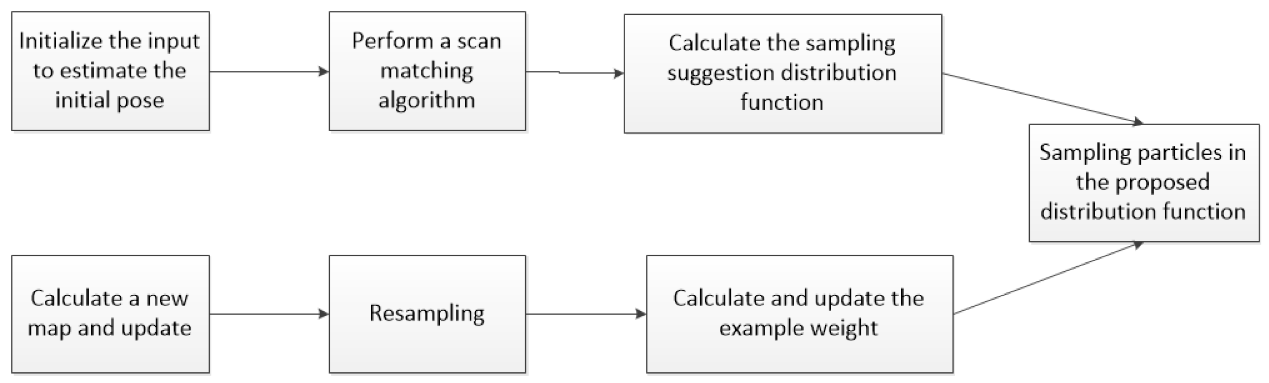By dividing the map into grids, Gmapping can efficiently deal with large-scale environments, and because of the use of particle filtering technology, it also performs well in nonlinear and dynamic environments, making it an important tool in the field of autonomous navigation and map building [18]. At the same time, for the particle dissipation problem, an adaptive resampling strategy is put forward to improve computational efficiency. The Gmapping algorithm encompasses several key steps in Simultaneous Localization and Mapping (SLAM) [19]. It begins by initializing the input to estimate the robot’s initial pose, incorporating position and orientation. Through a scan matching algorithm, the current sensor readings are compared with the existing map, refining the robot’s pose estimation. A sampling suggestion distribution function is then calculated, guiding the selection of new particles for resampling. These particles contribute to the calculation of a new map, subsequently updated based on the likelihood of observed sensor data. Resampling ensures the retention of probable poses, and weights are assigned to particles according to their agreement with the sensor data. The algorithm iteratively refines the robot’s pose estimation and updates the map, providing a probabilistic framework for effective SLAM in dynamic and unknown environments [20]. The principle of the algorithm is shown in Figure 1.

2.1. RBPF SLAM

The RBPF-SLAM algorithm employs a clever method to decompose the Simultaneous Localization and Mapping (SLAM) problem into two key sub-problems: the localization of the robot itself and the location estimation of the environmental features [21]. This idea of splitting helps us deal with this complex task more effectively [22]. First, the particle filter algorithm is utilized to estimate the robot’s position along the entire path by tracking many particles, thereby achieving high-precision positioning of the robot. Then, the extended Kalman filter algorithm is applied to establish an independent EKF for each environmental feature to estimate its position. This step transforms the location estimation problem of environmental features into a series of relatively simplified sub-problems; each EKF corresponds to a specific environmental feature. Through this decomposition and combination method, the SLAM problem can be solved more effectively, the accuracy and robustness of positioning and map construction can be improved, and the state space dimension during sampling can be reduced to simplify the calculation [23].

The implementation process of the RBPF algorithm is as follows:

(1) Sampling: According to the suggested distribution, samples are taken from the particle set at time t − 1 to obtain the prior distribution set of particles at time t. In this process, it is recommended that the distribution adopts the robot’s motion model, which describes the robot’s motion between time t − 1 and time t to help predict the new particle state. This step allows us to generate new candidate particles based on the prediction of the motion model in SLAM (Simultaneous Localization and Mapping) to update the robot’s position and map construction.

(2) Calculate the weight: By calculating the weight of each particle, the contribution of each particle to the estimation process can be quantified. These weights reflect the difference between the proposal distribution and the target posterior distribution. This measure of the degree of difference helps to determine the relative contribution of each particle, making it more focused on the particles that are more important for problem solving when estimating the posterior distribution of the target. This is a process based on the importance sampling principle, in which the weight of the first particle is used to indicate its relative importance in estimating the posterior distribution of the target, thereby helping to improve the accuracy and effectiveness of the estimation. The formula for calculating particle weight can be expressed as follows:

$${\tilde{\omega }}_t^{\left(i\right)}=\frac{p\left(x_{1:t}^{\left(i\right)}\left|z_{1:t}^{\left(i\right)}\right.,c_{1:t-1}^{\left(i\right)}\right)}{\Pi \left(x_{1:t}^{\left(i\right)}\left|z_{1:t}^{\left(i\right)}\right.,c_{1:t-1}^{\left(i\right)}\right)}$$

(1)

In the formula, $w$ is the particle weight, $p$ is the posterior probability, the observed value is $z_{1:t}=z_1,z_2,z_3,\dots ,z_t$ , the estimated trajectory of the robot is $x_{1:t}=x_1,x_2,x_3,\dots ,x_t$ , and the control quantity is $c_{1:t}=c_1,c_2,c_3,\dots ,c_t$ .

(3) Resampling: By resampling according to the weight of each particle, we select and extract M particles from the temporary particle set. This process aims to retain the particles with higher weights to ensure that they occupy a greater proportion in the new particle set. New M particles will be generated through this resampling process, forming a new final particle set. The set, after being subjected to weighted sampling, more accurately reflects the importance of the particles and contributes to the enhancement of performance and accuracy within the SLAM system.

(4) Update the map: For each particle, the map is updated in real time by combining the sensor observation data and the current pose information of the robot, especially for each feature object in the map. This process allows each particle to track and update the feature objects in the map in the SLAM system to continuously improve the accuracy and detail of the map, thereby improving the robot’s autonomous navigation and map construction capabilities in an unknown environment.

2.2. Grid Map

Grid mapping is the most widely used mapping technique in the current field of robotics. It divides the surrounding environment into multiple grids, with each grid storing occupancy or elevation information. For typical scenarios, a two-dimensional grid map is commonly used, where the color of each grid cell represents the state of that area [24].

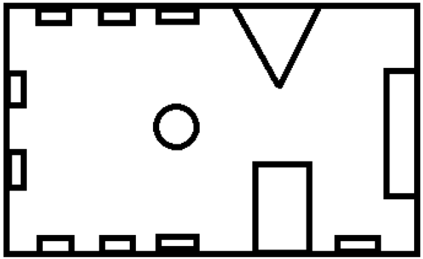
As shown in Figure 2, the black areas represent indoor boundaries, rectangular and triangular obstacles, and double-layered logistics sorting stations. White areas indicate open spaces that have been explored indoors, while dark gray areas represent spaces not detected by the laser radar.

For each grid, $p(s=1)$ represents the probability of being in a free state, while $p(s=0)$ represents the probability of being in an occupied state. The sum of these probabilities equals 1. Here, $s$ denotes the grid, and $z$ represents the radar observation. By using the ratio of probabilities between the two states to denote the current state of the grid, it can be expressed as

$$Odd(s)=\frac{p(s=1)}{p(s=0)}$$

(2)

When the observation value (z~{0,1}) of the lidar is updated, the corresponding grid immediately updates the grid state to be

$$Odd(s|z)=\frac{p(s=1|z)}{p(s=0|z)}$$

(3)

Here, $p(s=0|z)$ represents the probability of being in a free state given z, while $p(s=1|z)$ represents the probability of being in an occupied state given z. This equation can be likened to a conditional probability problem, where $Odd(s|z)$ represents the state of the grid given the occurrence of z.

Based on Bayes’ theorem, the following two equations are derived:

$$p(s=1|z)=\frac{p(z|s=1)p(s=1)}{p(z)}$$

(4)

$$p(s=0|z)=\frac{p(z|s=0)p(s=0)}{p(z)}$$

(5)

Substituting the above equations into Equation (3) yields

$$\left\{\begin{array}{c}Odd(s|z)=\frac{p(s=1|z)}{p(s=0|z)}\\ Odd(s|z)=\frac{p(z|s=1)p(s=1)}{p(z|s=0)p(s=0)}\\ Odd(s|z)=\frac{p(z|s=1)}{p(z|s=0)}\ast \frac{p(s=1)}{p(s=0)}\\ Odd(s|z)=\frac{p(z|s=1)}{p(z|s=0)}\ast Odd(s)\end{array}\right.$$

(6)

By taking the logarithm of both sides of the equation, we obtain

$$logOdd(s|z)=log\frac{p(z|s=1)}{p(z|s=0)}+logOdd(s)$$

(7)

This equation represents another change in the grid state, denoted by $logOdd(s)$ for a single grid. Now, in this equation, the term involving the measurement is denoted by $log\frac{p(z|s=1)}{p(z|s=0)}$ , which is referred to as the measurement model. The observation state for a grid by the laser radar is either occupied or free, as shown in Equation (8).

$$\left\{\begin{array}{c}lofree=log\frac{p(z=0|s=1)}{p(z=0|s=0)}\\ looccu=log\frac{p(z=1|s=1)}{p(z=1|s=0)}\end{array}\right.$$

(8)

We can use $logOdd(s)$ to represent the state $s$ of grid S. Therefore, we can further simplify the update rules for the grid map to

$$S^{+}=S^{-}+log\frac{p(z|s=1)}{p(z|s=0)}$$

(9)

Here, $S^{+}$ and $S^{-}$ respectively represent the state of grid \(s\) after and before the measurement.

2.3. Resampling Strategy

To efficiently manage computational resources and reduce particle depletion, the Gmapping algorithm introduces an important threshold mechanism [25]. The core idea of this strategy is to perform resampling only when it falls below a set threshold; otherwise, it remains unchanged. This implies that particles deemed important are not frequently replaced, effectively enhancing computational efficiency and algorithm stability. This mechanism introduces more intelligent management into the filtering process of Gmapping, enabling better adaptation to dynamic environments and resource utilization demands. Considering that resampling occurs in each iteration, this not only wastes computational resources but also leads to particle depletion. The threshold for resampling can be expressed as

$$N_{eff}=\frac{1}{{\displaystyle {\displaystyle \sum }_{i=1}^N}{\left({\tilde{\omega }}_t^{\left(i\right)}\right)}^2}$$

(10)

where $N_{eff}$ represents the resampling threshold, and ${\tilde{\omega }}^{(i)}$ represents the normalized weight of the $i$-th particle.

2.4. Gmapping Algorithm Flow

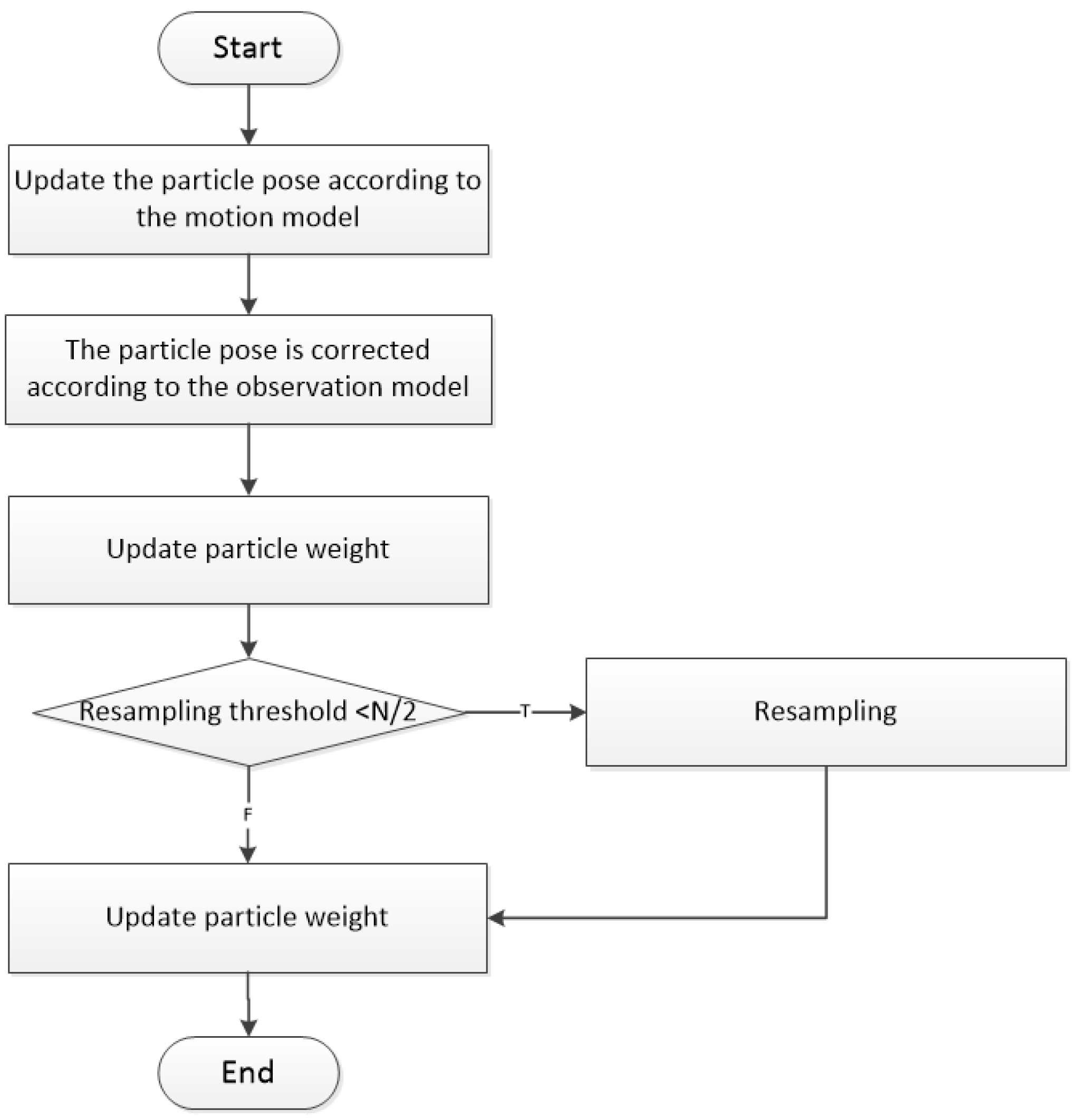
The Gmapping algorithm initially estimates the real-time location of the robot using probabilistic filtering techniques, and then it effectively represents and constructs an environment map using grid maps. In each iteration loop, Gmapping performs laser data updates, aiding in estimating the robot’s position and updating the map of the surrounding environment [26]. Crucially, the algorithm also introduces an importance threshold mechanism, allowing resampling only when the importance of the particles falls below a predefined threshold. This enhances computational resource utilization efficiency and reduces particle dissipation. Gmapping stands out for its efficient adaptation to dynamic environments, simultaneously achieving localization and map construction. As a result, it finds widespread application in solving problems related to autonomous navigation and SLAM. The Gmapping algorithm operates through a series of steps to enable Simultaneous Localization and Mapping (SLAM). Initially, the algorithm constructs the map with the robot’s initial position and orientation. Subsequently, the robot employs a laser rangefinder to scan the surrounding environment, updating its motion model based on odometry data. The measurement model is then updated by comparing the laser data with the existing map, establishing data associations, and refining the map’s occupancy status. Through particle filtering, weights are assigned to particles based on their agreement with the observed sensor data, facilitating resampling to retain more probable particles. The algorithm iteratively refines the robot’s pose estimation, updates the map, and outputs a refined map and the robot’s current position. The algorithm’s workflow is depicted in Figure 3.

3. Visual Odometry

Visual odometry (VO), an essential perception technology, finds widespread application in fields like mobile robotics and autonomous driving vehicles. Its core task involves estimating the camera’s motion in the world coordinate system by processing consecutive frames of images, enabling autonomous navigation and localization [27].

The working principle of visual odometry is based on computer vision and image processing techniques. This principle determines the camera’s motion in three-dimensional space by analyzing feature points or descriptors in adjacent image frames, such as corners, edges, or ORB features. By tracking the positional changes of these feature points across different image frames, VO computes the camera’s pose changes, encompassing translation and rotation [28].

Visual odometry finds extensive application in areas including autonomous driving vehicles [29], drones, robots, and more. It is utilized in these domains for real-time autonomous navigation and localization, aiding in obstacle avoidance, path planning, task execution, etc. Additionally, VO can be combined with data from other sensors like Inertial Measurement Units (IMUs) or Global Positioning Systems (GPSs) to enhance the accuracy and robustness of localization. The implementation steps are as follows:

(1) Feature Extraction: Extracting feature points from consecutive image frames is a computer vision technique used to identify and mark prominent key points within images. These feature points are typically local areas within the image, such as corners (vertices), edges, or regions with texture variations, possessing unique discernible properties across different images.

(2) Feature Matching: By comparing feature points in adjacent image frames, the system establishes correspondences between them, achieving key point matching. This matching process relies on feature descriptors like SIFT or ORB. Scale-Invariant Feature Transform (SIFT) is a computer vision algorithm designed for detecting and describing key feature points in images. It achieves this by filtering the image at different scales and orientations, extracting features that are insensitive to scale and rotation changes. SIFT finds widespread application in areas such as image matching and object recognition due to its high robustness to variations in images. ORB (Oriented FAST and Rotated BRIEF) is a feature detection and description algorithm commonly used in computer vision. It combines the efficiency of the FAST key point detector with the robustness of the BRIEF descriptor, providing a fast and reliable method for feature extraction in image processing tasks like object recognition and tracking. It provides a numerical representation to describe the appearance and structural features of each feature point. It enables the system to determine correspondences precisely and reliably between feature points across different frames.

(3) Motion Estimation: By leveraging the correspondences of feature points, the system estimates the camera’s relative motion between two consecutive image frames. This relative motion typically includes the estimation of a translation vector (describing the camera’s displacement) and a rotation matrix (describing the camera’s pose transformation).

The translation vector describes the displacement and direction of the camera from one image frame to the next. By comparing the positional differences of corresponding feature points between frames, the system computes the camera’s translation vector. This often involves utilizing matched feature points to estimate relative displacement, aligning one frame with another through translation correction. The rotation matrix describes the camera’s rotation from one frame to another. By analyzing the relative directional differences between corresponding feature points, the system estimates the camera’s rotation matrix, allowing content in one frame to be rotated to match that in another frame, achieving precise image alignment.

(4) Integration and Accumulation: By using estimates of relative motion, the system estimates the camera’s global motion cumulatively. This involves accumulating the camera’s motion at each time step (typically represented by translation vectors and rotation matrices) to derive the camera’s trajectory. This cumulative approach enables the system to track the camera’s movement from its initial position to its current position, considering both transitional and rotational motion at each time step to construct the camera’s global motion path.

(5) Scale Estimation: Visual odometry cannot directly estimate scale (actual object distances), requiring additional information for scale estimation. This can be achieved through data provided by other sensors (like LiDAR or GPS). LiDAR offers precise 3D point cloud information about the camera’s location, aiding in determining scale. GPS provides global position information for large-scale localization [30]. The fusion of visual odometry data with information from these sensors allows for a more accurate scale estimation. Another approach involves using specific scene features to estimate scale, such as identifying and tracking specific objects or markers in the scene, like traffic signs, ground markings, or objects of known sizes. Measuring the pixel distances of these features in images allows them to be mapped to real-world scales. This method often requires scene modeling and pre-measurement.

(6) Error Optimization: In practical applications, the estimated results might be influenced by various factors, including noise and cumulative errors. To enhance trajectory estimation accuracy, optimization techniques are typically employed, with bundle adjustment being a common approach. Bundle adjustment aims to improve the estimation of camera trajectories by minimizing estimation errors and achieving more accurate results.

4. Laser Radar Data Preprocessing

Mobile robots utilize LiDAR technology for external environment perception [31]. LiDAR enables pose estimation and the construction of 2D maps for mobile robots [32] through the processing of scanned data [33]. In this technology, the forward direction of the 2D LiDAR is defined as the polar axis, while the rotation center of the LiDAR ranging core is set as the pole, establishing a polar coordinate system. The data obtained by the 2D LiDAR in the form of point clouds can be represented as

$$N=\left\{\left({\lambda }_1,{\phi }_1\right)|i=1,2,3,\dots .,n\right\}$$

(11)

In the equation, $N$ represents the collected LiDAR point cloud data, ${\lambda }_1$ stands for the distance detected by the LiDAR for the $i$-th set of point cloud data, and ${\phi }_1$ denotes the fixed angle detected by the LiDAR for the $i$-th set of point cloud data.

The polar coordinate representation form of the pair (11) is converted to the rectangular coordinate representation form, and the conversion formula is

$$\left\{\begin{array}{c}{x}_i={\lambda }_i\cos {\phi }_i\\ y_i={\lambda }_i\sin {\phi }_i\end{array}\right.$$

(12)

In the equation, $x_i$ represents the x-axis coordinate value in the Cartesian coordinate system for the $i$-th set of point cloud data, $y_i$ stands for the y-axis coordinate value in the Cartesian coordinate system for the $i$-th set of point cloud data, and ${\phi }_i$ denotes the fixed angle detected by the $i$-th set of point cloud data.

The transformed point cloud data collected by the LiDAR can be represented as

$$N=\left\{\left(x_i,y_i\right)i=1,2,3,\dots .,n\right\}$$

(13)

In the equation, $N$ represents the point cloud dataset, $x_i$ stands for the x-axis coordinate value in the Cartesian coordinate system for the $i$-th set of point cloud data, and $y_i$ denotes the y-axis coordinate value in the Cartesian coordinate system for the $i$-th set of point cloud data.

During the motion of a mobile robot, crucial information is acquired through LiDAR technology, which is used to capture various observational data, including measurements of distance and angular orientation between objects and the mobile robot itself. These observations play a vital role in the navigation, localization, and environmental perception of the mobile robot. Therefore, the observational quantity of a mobile robot can be represented in the following manner:

(1) Distance Observation: This represents measurements of the distance between objects and the mobile robot. This information provides the relative positions of objects within the environment, aiding the robot in path planning for obstacle avoidance and distance estimation.

(2) Angular Observation: This represents the angle between objects and the robot’s coordinate system. Typically used to determine the orientation of objects relative to the robot, it allows the robot to track targets or rotate itself to adapt to the environment.

Thus, the observational quantity of a logistics sorting robot can be represented as

$$M={\left[p,w\right]}^T$$

(14)

In the equation, $M$ represents the observational quantity of the logistics sorting robot, $p$ stands for the distance between the object being measured and the robot, and $w$ denotes the angular velocity.

The pose of a mobile robot moving on a plane can usually be described by a plane position coordinate $\left(X,Y\right)$ and a rotation angle $\theta$ (representing direction or angle), forming a three-dimensional vector ${\left(X,Y,\theta \right)}^T$ , where $X$ and $Y$ represent the position coordinates of the robot on the plane, and a represents the orientation or rotation angle of the robot. Then, the observation model obtained by the $i$-th laser of the mobile robot at time t can be expressed as

$$M_i\left(t\right)=H\left(X_r\left(t\right)\right)+{\eta }_i\left(t\right)$$

(15)

where is the abstract function of time $t$ , $X_r\left(t\right)$ is the position of the mobile robot at time $t$ , and ${\eta }_i\left(t\right)$ is the noise of the sensor at time $t$ .

The two-dimensional lidar sensor can obtain two key observations between the measured object and the mobile robot itself during the scanning process: distance ($p$) and angle ($\theta$). The distance observation represents the distance between the measured object and the robot itself, measured by the lidar. Each laser beam will return a distance observation value, which reflects the distance between the object and the robot. Distance observation is usually measured in meters. The angle observation represents the direction angle of the laser beam, which is usually described relative to the robot’s coordinate system or the global coordinate system. Therefore, the observation model during the scanning process can be expressed as

$$M_i\left(t\right)=\left[\begin{array}{c}{p}_i\left(t\right)\\ w_i\left(t\right)\end{array}\right]=\left[\begin{array}{c}\sqrt{{\left(x_i-x_r\left(t\right)\right)}^2+{\left(y_i-y_r\left(t\right)\right)}^2}\\ \arctan \left(\frac{y_i-Y\left(t\right)}{x_i-X\left(t\right)}\right)-\theta \left(t\right)\end{array}\right]+{\eta }_i\left(t\right)$$

(16)

In the formula, $M_i\left(t\right)$ is the observation model obtained by the I-beam laser logistics sorting robot at time $t$ , $p_i\left(t\right)$ is the distance between the I-beam laser at time $t$ and the robot, $w_i\left(t\right)$ is the angular velocity when the I-beam laser at time t is detected, $\theta \left(t\right)$ is the angle between the measured object and the mobile robot at time $t$ , $x_r\left(t\right)$ is the coordinate value of the logistics sorting robot in the x-axis direction at time $t$ , and $y_r\left(t\right)$ is the coordinate value of the logistics sorting robot in the y-axis direction at time $t$ . 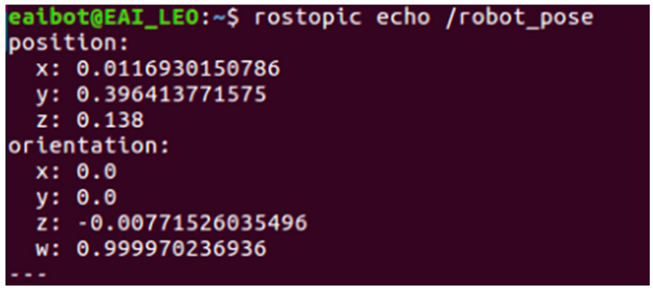Figure 4 shows the coordinates converted by the car at a certain position during the experiment.

5. Monocular Camera Coordinate Transformation

Before using machine vision measurement technology for high-precision measurement, camera calibration is first performed to obtain the internal and external parameters of the camera [34]. The camera involves the world coordinate system $\left(X_w,Y_w,Z_w\right)$ , camera coordinate system $\left(X_s,Y_s,Z_s\right)$ , imaging coordinate system $\left(x,y\right)$ , and pixel coordinate system $\left(u_0,v_0\right)$ in the process of imaging transformation. To determine the position of the camera in space, the coordinate position is transformed from the world coordinate system to the camera coordinate system through the rotation matrix, $R$ , and the translation matrix, $T$ . The transformation between the two coordinate systems is

$$\left[\begin{array}{c}{X}_s\\ Y_s\\ Z_s\end{array}\right]=R\left[\begin{array}{c}{X}_w\\ Y_w\\ Z_w\end{array}\right]+T$$

(17)

In the formula, $R$ is a 3 × 3 orthogonal unit matrix, and $T$ is a 3 × 1 shift matrix.

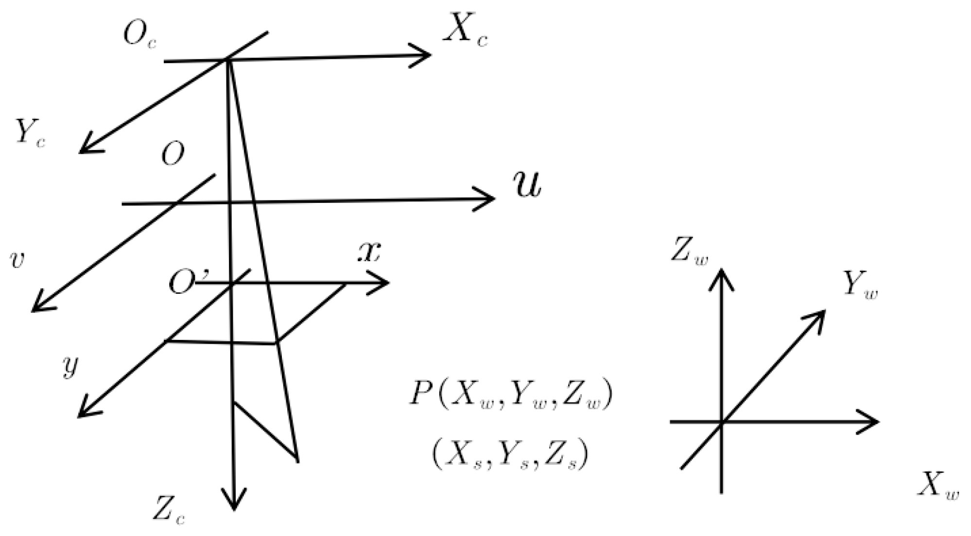
In the process of imaging, four different coordinate systems are involved, which play a vital role in capturing and analyzing the position and shape information of objects. The object coordinate system represents the position of the object in three-dimensional space and provides the coordinate information of the object in the real world [35]. The camera coordinate system is relative to the object coordinate system, and it describes the position and direction of the camera or imaging device and provides a reference frame for subsequent imaging. The imaging plane coordinate system is a coordinate system representing the pixel coordinates on the image plane, and it provides a tool for measuring the position of the object in the image. There is a key projection relationship between the camera coordinate system and the imaging plane coordinate system. This relationship defines how the actual point of the object is mapped to the imaging point, which is usually achieved by perspective projection or affine transformation. These four coordinate systems and the projection relationship between them are of great significance in the fields of computer vision and image processing. The projection relationship between the actual point of the object and the imaging point is shown in Figure 5.

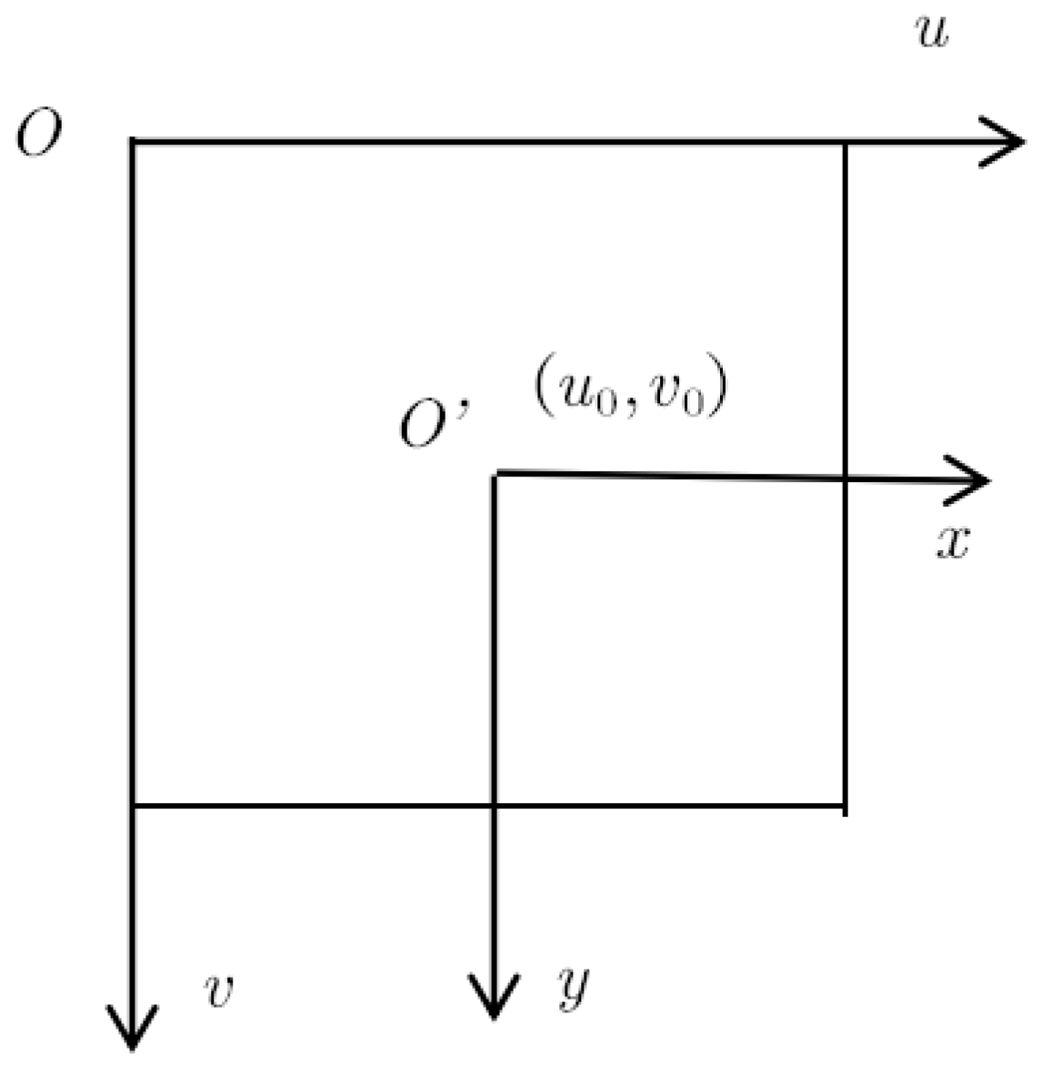
In image processing, the image coordinate unit in the image physical coordinate system is a millimeter, while in the image pixel coordinate system, the image coordinate unit is a pixel. The two coordinate systems are located on the same plane, and the relationship between them is shown in Figure 6, which describes the mapping and connection between them in detail. This transformation relationship between coordinate systems is of great significance in the field of image processing and computer vision, and it is used to accurately measure and analyze the position and size information in the image.

If the homogeneous coordinate of a point in space in the world coordinate system is $\left(X_w,Y_w,Z_w,1\right)$ , and the homogeneous coordinate in the camera coordinate system is $\left(X_s,Y_s,Z_s,1\right)$ , according to the standard transformation relationship in the field of image processing and computer vision, the transformation between the pixel coordinate system and the world coordinate system can be expressed as

$$Z_s\left[\begin{array}{c}u\\ v\\ 1\end{array}\right]=\left[\begin{array}{cccc}c& 0& u_0& 0\\ 0& d& v_0& 0\\ 0& 0& 1& 0\end{array}\right]\left[\begin{array}{cc}R& T\\ O^T& 1\end{array}\right]\left[\begin{array}{c}{X}_w\\ Y_w\\ Z_w\end{array}\right]$$

(18)

In the formula, $c=fldx$ , $d=fldy$ represents the equivalent focal length. $f$ is the focal length; $dx$ and $dy$ are the physical sizes of each pixel in the x-axis and y-axis directions of the imaging coordinate system, respectively. $\left(u_0,v_0\right)$ is the optical center coordinate; $O$ is a 3 × 1 zero matrix.

Most optical systems have imperfections in the imaging process, which will lead to the distortion of the captured image [36]. When considering radial distortion and centrifugal distortion, there is a specific relationship between the coordinates of the actual object and the coordinates under ideal conditions [37]. The relationship between the two can be expressed as

$$RK=D$$

(19)

In the formula, $R$ is the real coordinate, $K$ is the conversion coefficient, and $D$ is the ideal coordinate.

Real coordinates, transformation coefficients, and ideal coordinates can be expressed as

$$R={\left[\begin{array}{cc}x{r}^2& y{r}^2\\ x{r}^4& y{r}^4\\ x{r}^6& y{r}^6\\ \left(2x^2+r^2\right)& 2xy\\ 2xy& \left(r^2+2y^2\right)\end{array}\right]}^T$$

(20)

$$K=\left[l_1 l_2 l_3 t_1 t_2\right]$$

(21)

$$D=\left[\begin{array}{c}{u}_0-u\\ v_0-v\end{array}\right]$$

(22)

where $r^2=x^2+y^2$ denotes the square of the distance from any point in the image to the center of the distortion. $x=u-u_0$ , $y=v-v_0$ , $\left(u,v\right)$ is the ideal image position. $\left(u_0,v_0\right)$ is the actual image position; $l_1 ,l_2 \mathrm{and} l_3$ are the radial distortion coefficients. $t_1 \mathrm{and} t_2$ are the tangential distortion coefficients. Figure 7 shows the adjustment of the robot camera distortion during the experiment.

6. Experimental Process and Result Analysis

6.1. Experimental Schematic Design

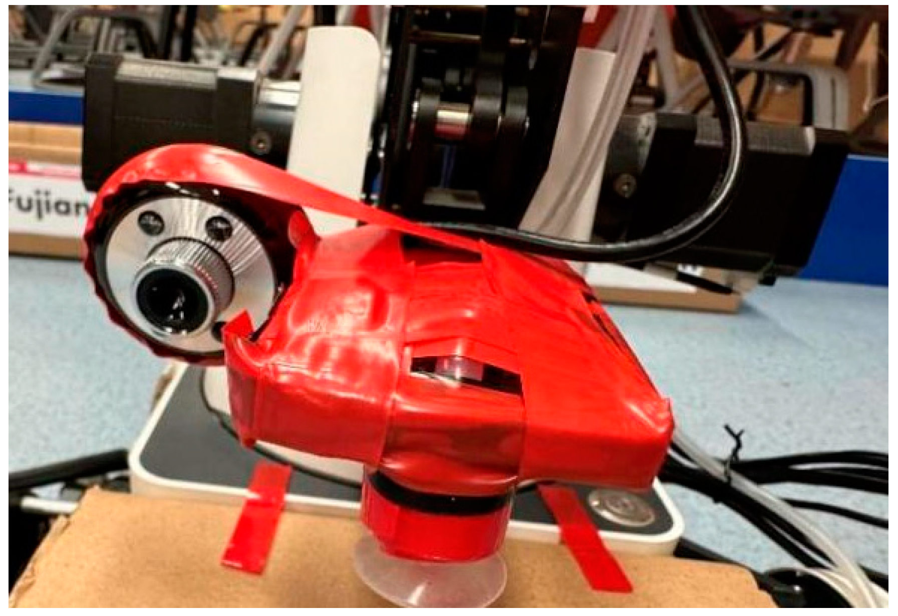
An LEO mobile robot is used as the mobile platform, equipped with a variety of key sensors, including an EAI G1 laser radar and an Obi mid-light depth camera. These sensors work together to allow LEO robots to achieve high-precision map construction, obstacle perception, and autonomous navigation in different environments, providing powerful perception capabilities for adapting to various application scenarios, as shown in Figure 8.

The EAI G1 laser radar has unique performance characteristics, such as an angular resolution, maximum ranging distance, and accuracy, while the Obi mid-light depth camera has high-resolution depth perception capabilities. The combined application of these two sensors provides robots with comprehensive sensing data, enabling them to efficiently perceive the surrounding environment, perform map construction, and perform complex navigation tasks.

Table 1. The specific parameters of EAI G1 laser radar.

Parameter	Value
Location principle	Range of triangle
Angle resolution	0.5 degrees
Maximal detectable range	15 m
Accuracy of ranging	−1%–+1%

and

Table 2. Obi middle light depth camera-specific parameters.

Parameter	Value
Type	Obi middle light mini
Ranging distance	0.4 m–2 m
Range of angles	Upward 16 degrees elevation angle Downward 24 degrees pitch angle 24.5 degrees wide angle left and right
Maximum sample rate	25 Hz

show the specific parameters of the radar and camera, respectively.

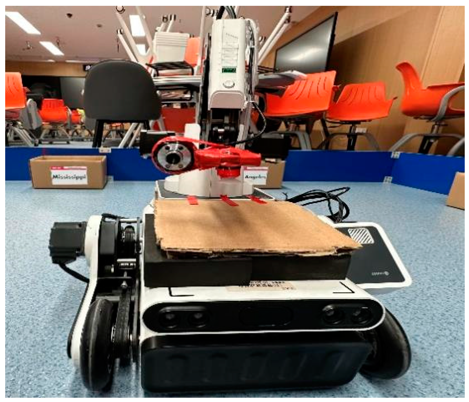
The upper computer of the robot uses a Huawei laptop, equipped with the Ubuntu 18.04 operating system, and it has the ROS (Robot Operating System) software (V1.0) platform installed. The overall height of the robot is 0.42 m. This configuration enables the robot to have powerful computing and control capabilities, providing a stable operating environment and software support for various robot applications. Figure 9 shows the logistics sorting robot used in the experiment.

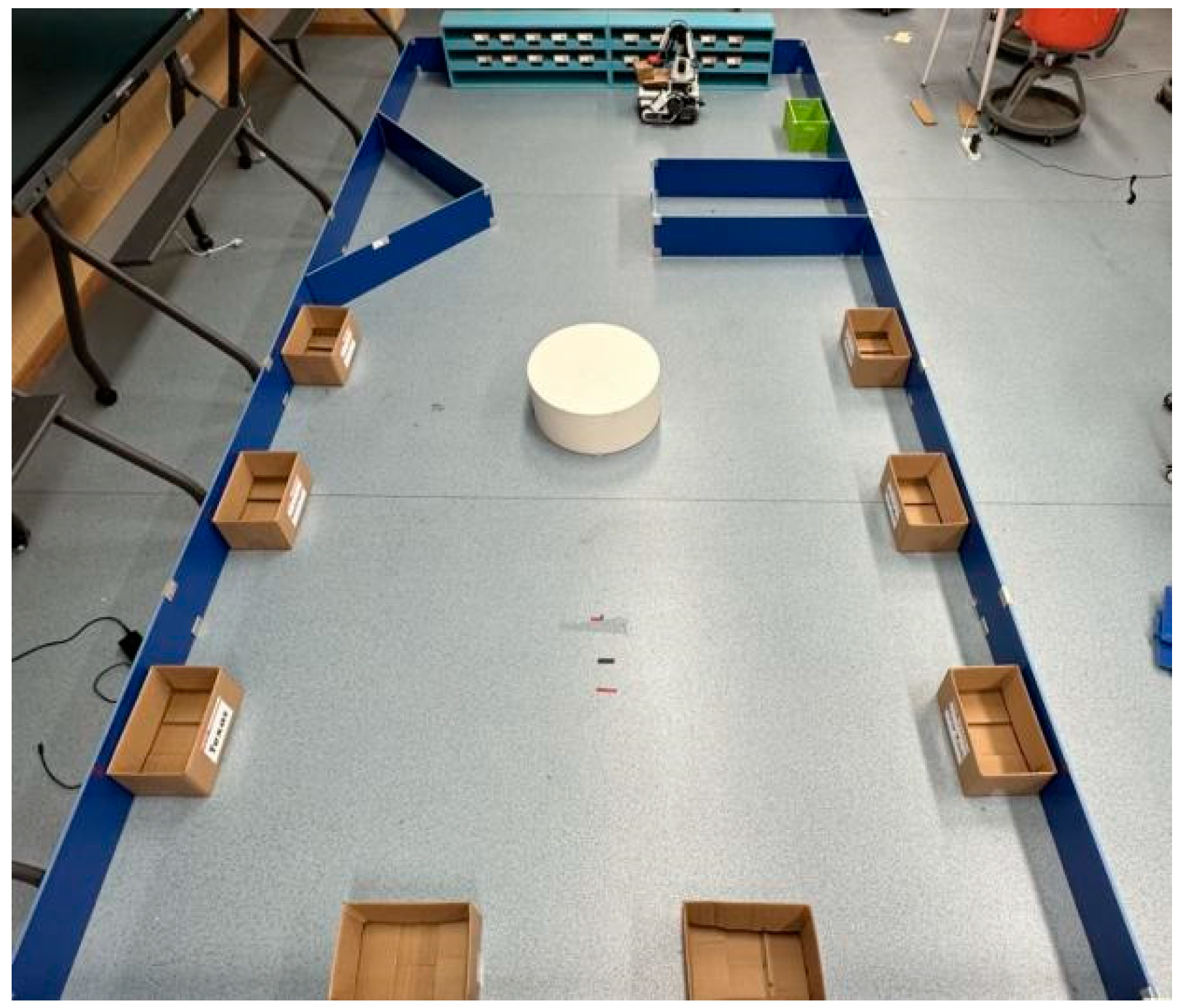
The warehouse environment simulation experiment site is 5.12 m long and 2.51 m wide, providing a spacious working space suitable for various navigation experiments and obstacle avoidance application scenarios, allowing for diverse testing, research, and experiments. The specific experimental site is shown in Figure 10.

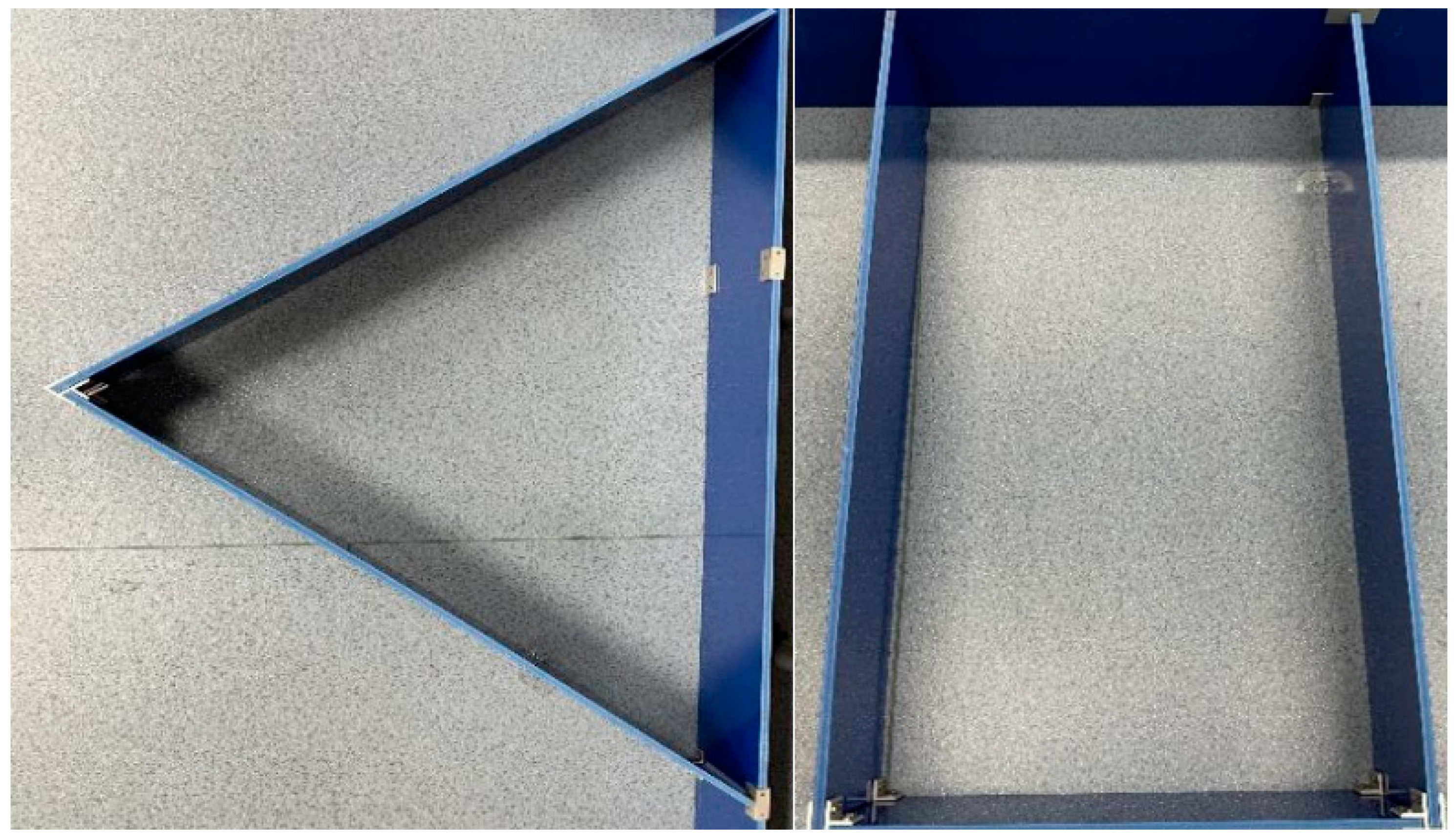
Objects of various shapes and sizes are placed on the site to simulate the complex environment of the logistics warehouse and provide rich experimental conditions. Specifically, they include triangular obstacles with three sides of 100.3 cm, 101.85 cm, and 20.05 cm and rectangular obstacles with a length of 100.35 cm, a width of 53.92 cm, and a height of 20 cm. This diversity of obstacle shapes and sizes provides conditions closer to those of practical applications for logistics navigation and obstacle avoidance experiments, enabling research to more comprehensively evaluate and improve the performance of logistics vehicles. The specific experimental site obstacles are shown in Figure 11.

6.2. Analysis of the Effect

To present the significant advantages of the Gmapping algorithm more fully in guiding sorting robots to avoid obstacles in logistics warehouses, the researchers carry out several performance evaluations, which include a measurement of the mapping time and an evaluation of the obstacle detection rate and accuracy to ensure the efficient construction of the map and verify its reliability in identifying obstacles. At the same time, a quantitative analysis of the size and angle accuracy of the map is carried out to ensure that the generated map matches the actual environment. These comprehensive performance indicators enable the researchers to fully analyze the practical application value of the improved Gmapping algorithm in the navigation of logistics sorting robots.

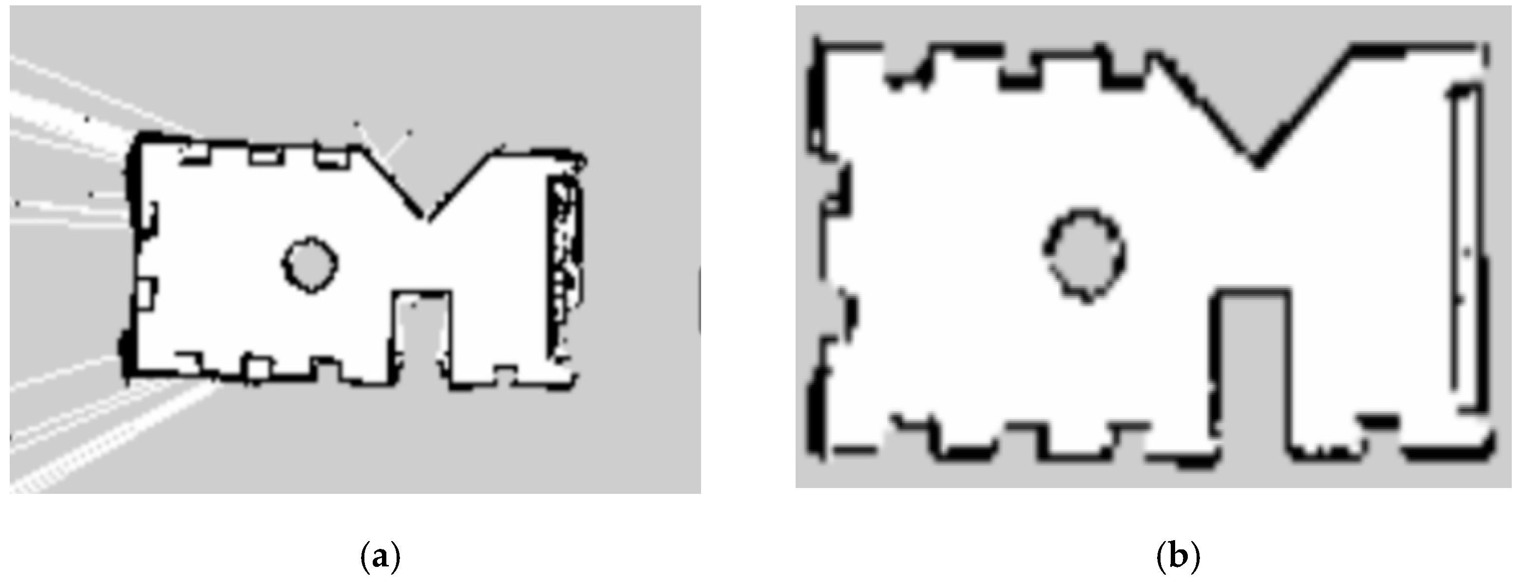
Figure 12 shows the reference map obtained from the actual measurement. Figure 13a shows the grid map established by the Gmapping algorithm, and Figure 13b shows the grid map established by the improved Gmapping algorithm in this research. From the mapping results, it can be observed that the original Gmapping algorithm has problems such as overlapping and confusion in the edge areas of the map and the incomplete detection of some obstacles. The map generated by the improved algorithm is clearer and neater than the map of the original Gmapping algorithm, and the edges do not overlap, thus more accurately reflecting the real environment and providing more reliable map data.

(1) Mapping time and obstacle detection rate

To obtain stable mapping time data, 15 map constructions are carried out, and the average time is calculated. In addition, the obstacle detection rate $f$ is set, which represents the ratio of obstacles successfully detected in the map established by the sensor. By measuring the total side length $S_1$ of the obstacle detected in the map generated by the sensor, a quantitative index of the obstacle detection accuracy can be obtained. At the same time, to verify the accuracy of the map, the total side length $S_2$ of the actual obstacle is referenced, which provides an important measure of the map accuracy. By comparing the obstacle side length $S_1$ in the map generated by the sensor with the obstacle side length $S_2$ in the actual environment, the performance of the Gmapping algorithm in construction and obstacle detection can be evaluated to ensure that the robot can reliably avoid obstacles in the logistics warehouse.

$$f=S_1/S_2$$

(23)

The obstacle detection rate and mapping time are shown in

Table 3. Obstacle detection rate and mapping time.

Parameter	Gmapping Algorithm	Improved Algorithm
Obstacle detection rate/(%)	92.26	96.31
Mapping time/(s)	196	187

.

In the experiments conducted in Table 3, the performance of the Gmapping algorithm in obstacle detection is 92.26%, and the average time required for mapping is 196 s. However, the improved algorithm significantly improves the obstacle detection rate and maintains high efficiency in mapping speed. The average mapping time is only 187 s.

(2) Accuracy of walking distance

To evaluate the accuracy of the car’s walking distance, the actual distance of the car’s walking is measured three times, and these actual distances are compared with the values of the car’s wheeled odometer. By comparing the actual measured distance and the distance estimated by the odometer, the accuracy of the car’s walking distance is calculated. This process helps to analyze the accuracy and error level in the movement of the car, which helps to better understand and improve the performance of the navigation system. The measurement results are shown in

Table 4. Accuracy measurement of odometer.

Parameter	Actual Measuring	Gmapping Value	Improved Algorithm Mapping Value
First walking distance/cm	100	95.3	97.3
Second walking distance/cm	50	47.7	47.9
Third walking distance/cm	100	94.6	99.5
Average error/(%)		4.9	2.5

.

It can be seen in Table 4 that the accuracy error of the Gmapping algorithm in the wheel odometer is 4.9%. When estimating the position and direction of the robot, there is a big gap with the actual measured value, which may lead to inaccurate maps and trajectories in mapping and positioning. The improved algorithm has an error of 2.5% in terms of the accuracy of the wheel odometer, which reduces the gap between the actual measurement value and the actual measurement value and can more accurately estimate the position and direction of the robot.

(3) Map size accuracy and angle accuracy

To evaluate the dimensional accuracy and angular accuracy of the map, three line segments and three angles are selected for measurement and an error analysis. By measuring the actual length of these line segments and the corresponding length in the map and by measuring the actual angle and the corresponding angle in the map, the accuracy of the size and angle of the map can be determined. This process helps to identify possible scaling errors or rotation errors in the map and provides a relationship between the actual accuracy and modeling accuracy of the map. This detailed analysis helps to determine the applicability of the map, especially for applications such as autonomous navigation robots, to ensure that they can accurately navigate and avoid obstacles in the actual environment. The results of the measurement and error analysis are shown in

Table 5. Measurement results and error analysis.

Parameter	Actual Measuring	Gmapping Algorithm Value	Improved Algorithm Mapping Value
Line segment 1/m	5.105	5.305	5.225
Line segment 2/m	2.485	2.595	2.575
Line segment 3/m	1.018	1.095	1.075
Angle 1/(degree)	89.5	90.7	90.4
Angle 2/(degree)	132.6	135.2	134.7
Angle 3/(degree)	90.2	91.7	91.2
Average error of line segment (%)		5.2	3.8
Angular error average (%)		1.7	1.2

.

The map size accuracy error of the Gmapping algorithm is 5.2%, while the improved algorithm reduces it to 3.8%. This shows that the improved algorithm is more accurate in estimating the size of objects in the map. The angle accuracy of the Gmapping algorithm is 1.7%, while the improved algorithm increases it to 1.2%. The improved algorithm more accurately estimates the angle and direction of the objects in the map, which can help the robot better avoid obstacles and perform tasks. 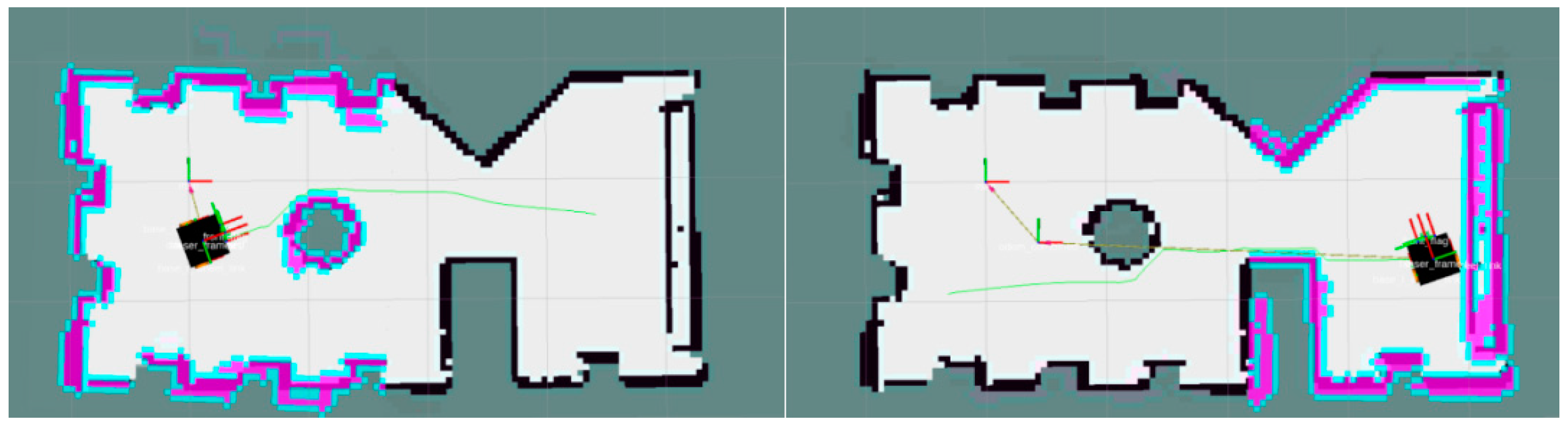Figure 14 and Figure 15 show the navigation processes of the Gmapping algorithm and the improved algorithm, respectively. The improved algorithm is more regular and clearer, which is conducive to the accurate identification of obstacles in the process of walking.

In summary, extensive empirical research was conducted by enhancing the Gmapping algorithm and comparing it with other relevant works in the current field. A set of standard validation metrics, including but not limited to obstacle detection rates, map size accuracy errors, and angle accuracy errors, was employed to ensure a comprehensive validation of the improved algorithm’s performance in various aspects. These metrics not only assessed the accuracy and robustness of the algorithm but also provided an objective basis for comparison with existing works. The experimental results, obtained by contrasting the performance of the improved algorithm with that of the traditional Gmapping algorithm, highlighted its significant advantages in high-resolution map construction and localization accuracy. These comparative results robustly support the effectiveness of the improved algorithm, ensuring that readers gain a comprehensive understanding of its performance and superiority.

Table 6. Comprehensive comparison of performance indicators for the improved algorithm.

Parameter	Gmapping Algorithm	Improved Algorithm
Obstacle detection rate/(%)	92.26	96.31
Mapping time/(s)	196	187
Accuracy of walking distance/(%)	95.1	97.5
Map size accuracy/(%)	94.8	96.2
angle accuracy/(%)	98.3	98.8

serves as a comprehensive comparison table of the performance indicators, vividly presenting the numerical differences detected in the experiments and highlighting the superior performance of the improved algorithm.

The improved algorithm demonstrates a high level of robustness in adapting to environmental color conditions. Its mapping process relies primarily on laser scan data provided by sensors; thus, it is unaffected by environmental colors. Therefore, whether indoors or outdoors, in bright or dim environments, the improved algorithm can accurately create maps. In terms of stability, the improved algorithm also exhibits satisfactory performance. It can effectively handle sensor data noise and uncertainty, maintaining map accuracy and continuity during long-term operation. Through optimization and parameter adjustments, we further enhance its stability to ensure reliable operation in various environmental conditions. Moreover, the improved algorithm demonstrates excellent adaptability, capable of adapting to diverse environments and scenarios. Whether indoors or outdoors, on flat terrain or complex terrain, the improved algorithm can efficiently perform map construction and path planning. Additionally, it can respond to changes in dynamic environments and promptly update map information to adapt to new circumstances.

7. Conclusions

Building upon the traditional Gmapping algorithm, this research integrates laser sensor data with visual odometry to craft a high-resolution grid map, significantly enhancing mapping and positioning accuracy. The improved algorithm significantly enhances obstacle detection rates, increasing them by 4.05%. Simultaneously, it successfully reduces map size accuracy errors by 1.4% and angle accuracy errors by 0.5%. Additionally, the accuracy of the robot’s travel distance improves by 2.4%, and the mapping time is reduced by nine seconds. The improvement made to the Gmapping algorithm, through the integration of laser sensor data with visual odometry, has significantly advanced map construction and localization accuracy. Simultaneously, it has had profound impacts on addressing diverse and complex logistics environments. The enhanced algorithm excels in constructing high-resolution maps, effectively capturing rich details within logistics warehouses. This enables robots to comprehensively and precisely perceive their surroundings, facilitating intelligent and efficient task execution in complex logistics scenarios. The collaborative effect of laser sensors and visual odometry enhances the adaptability of robots in different environments, enabling them to make rapid and accurate decisions, thereby increasing the flexibility of logistics sorting robots in complex environments. Moreover, the construction of high-resolution maps provides a solid foundation for various applications of other intelligent robots. For instance, in warehouse management, intra-warehouse transportation, and goods sorting, robots can accurately perceive and adapt to real-time changes within the warehouse, enhancing the overall efficiency and operability of the entire logistics system. This holds significant implications for the automation of logistics and the enhancement of supply chain efficiency.

The research not only positively impacts the field of logistics but also generates a series of significant effects in other domains. The enhanced accuracy in map construction and localization serves as a reliable foundation for the navigation of logistics robots, with potential applications in tasks such as automated warehousing, intra-warehouse transportation, and goods sorting, ultimately improving supply chain efficiency. Technological advancements also offer insights for intelligent traffic systems and urban planning, promoting the smart management of urban traffic, improving road utilization efficiency, and reducing traffic congestion. The continuous progress in robot technology is expected to drive the development of related industries, including the research and application of technologies such as laser sensors and visual odometry, fostering innovation and economic growth in these sectors.

There are still many challenges and opportunities in this field awaiting further study. The performance of visual odometry may vary under different environments and conditions, so more work is needed to improve its stability and adaptability. In addition, data fusion algorithms also need to be continuously improved to better integrate various sensor data.

References

- Xu, X.; Xue, Z.; Zhao, Y. Research on an Algorithm of Express Parcel Sorting Based on Deeper Learning and Multi-Information Recognition. Sensors 2022, 22, 6705. [Google Scholar] [CrossRef] [PubMed]
- Han, S.; Liu, X.; Han, X.; Wang, G.; Wu, S. Visual sorting of express parcels based on multi-task deep learning. Sensors 2020, 20, 6785. [Google Scholar] [CrossRef]
- Xue, T.; Li, L.; Shuang, L.; Zhiping, D.; Ming, P. Path planning of mobile robot based on improved ant colony algorithm for logistics. Math. Biosci. Eng. 2021, 18, 3034–3045. [Google Scholar] [CrossRef] [PubMed]
- Ma, J.; Yang, S.; Jing, H. Intelligent Warehouse Robot Scheduling System Using a Modified Nondominated Sorting Algorithm. Discret. Dyn. Nat. Soc. 2022, 2022, 2021535. [Google Scholar] [CrossRef]
- Zhao, Y.; Xie, K.; Liu, Q.; Li, Y.; Wu, T. Laser Based Navigation in Asymmetry and Complex Environment. Symmetry 2022, 14, 253. [Google Scholar] [CrossRef]
- Liu, H.; Zhou, L.; Zhao, J.; Wang, F.; Yang, J.; Liang, K.; Li, Z. Deep-Learning-Based Accurate Identification of Warehouse Goods for Robot Picking Operations. Sustainability 2022, 14, 7781. [Google Scholar] [CrossRef]
- Ren, C.; Ji, H.; Liu, X.; Teng, J.; Xu, H. Visual Sorting of Express Packages Based on the Multi-Dimensional Fusion Method under Complex Logistics Sorting. Entropy 2023, 25, 298. [Google Scholar] [CrossRef]
- Chen, Y.; Wu, J.; He, C.; Zhang, S. Intelligent Warehouse Robot Path Planning Based on Improved Ant Colony Algorithm. IEEE ACCESS 2023, 11, 360–12367. [Google Scholar] [CrossRef]
- Duan, L.; Liu, Y.; Li, H.; Park, K.H.; Cao, K. Nondominated Sorting Differential Evolution Algorithm to Solve the Biobjective Multi-AGV Routing Problem in Hazardous Chemicals Warehouse. Math. Probl. Eng. 2022, 2022, 3785039. [Google Scholar] [CrossRef]
- Wu, B.; Chi, X.; Zhao, C.; Zhang, W.; Lu, Y.; Jiang, D. Dynamic Path Planning for Forklift AGV Based on Smoothing A* and Improved DWA Hybrid Algorithm. Sensors 2022, 22, 7079. [Google Scholar] [CrossRef]
- Dong, L.; Yuan, X.; Yan, B.; Song, Y.; Xu, Q.; Yang, X. An Improved Grey Wolf Optimization with Multi-Strategy Ensemble for Robot Path Planning. Sensors 2022, 22, 6843. [Google Scholar] [CrossRef]
- Chen, T.; Chen, S.; Zhang, K.; Qiu, G.; Li, Q.; Chen, X. A jump point search improved ant colony hybrid optimization algorithm for path planning of mobile robot. Int. J. Adv. Robot. Syst. 2022, 19, 17298806221127953. [Google Scholar] [CrossRef]
- Yang, D.; Wu, Y.; Huo, D. Research on Design of Cross-Aisles Shuttle-Based Storage/Retrieval System Based on Improved Particle Swarm Optimization. IEEE Access 2021, 9, 67786–67796. [Google Scholar] [CrossRef]
- Honglin, Z.; Yaohua, W.; Jinchang, H.; Yanyan, W. Collaborative optimization of task scheduling and multi-agent path planning in automated warehouses. Complex Intell. Syst. 2023, 9, 5937–5948. [Google Scholar] [CrossRef]
- Achirei, S.D.; Mocanu, R.; Popovici, A.T.; Dosoftei, C.C. Model-Predictive Control for Omnidirectional Mobile Robots in Logistic Environments Based on Object Detection Using CNNs. Sensors 2023, 23, 4992. [Google Scholar] [CrossRef]
- Trejos, K.; Rincón, L.; Bolaños, M.; Fallas, J.; Marín, L. 2D SLAM Algorithms Characterization, Calibration, and Comparison Considering Pose Error, Map Accuracy as Well as CPU and Memory Usage †. Sensors 2022, 22, 6903. [Google Scholar] [CrossRef]
- Zhao, J.; Liu, S.; Li, J. Research and Implementation of Autonomous Navigation for Mobile Robots Based on SLAM Algorithm under ROS. Sensors 2022, 22, 4172. [Google Scholar] [CrossRef]
- Zhao, K.; Ning, L. Hybrid Navigation Method for Multiple Robots Facing Dynamic Obstacles. Tsinghua Science And Technology 2022, 27, 894–901. [Google Scholar] [CrossRef]
- Peng, G.; Zhou, Y.; Hu, L.; Xiao, L.; Sun, Z.; Wu, Z.; Zhu, X. VILO SLAM: Tightly Coupled Binocular Vision-Inertia SLAM Combined with LiDAR. Sensors 2023, 23, 4588. [Google Scholar] [CrossRef] [PubMed]
- Zhao, X.; Zuo, T.; Hu, X. OFM-SLAM: A Visual Semantic SLAM for Dynamic Indoor Environments. Math. Probl. Eng. 2021, 2021, 5538840. [Google Scholar] [CrossRef]
- Cai, Y.; Qin, T. Design of Multisensor Mobile Robot Vision Based on the RBPF-SLAM Algorithm. Math. Probl. Eng. 2022, 2022, 1518968. [Google Scholar] [CrossRef]
- Li, N.; Zhou, F.; Yao, K.; Hu, X.; Wang, R. Multisensor Fusion SLAM Research Based on Improved RBPF-SLAM Algorithm. J. Sens. 2023, 2023, 3100646. [Google Scholar] [CrossRef]
- Viset, F.; Helmons, R.; Kok, M. An Extended Kalman Filter for Magnetic Field SLAM Using Gaussian Process Regression. Sensors 2022, 22, 2833. [Google Scholar] [CrossRef]
- Cheng, C.; Wang, C.; Yang, D.; Liu, W.; Zhang, F. Underwater Localization and Mapping Based on Multi-Beam Forward Looking Sonar. Front. Neurorobotics 2022, 15, 801956. [Google Scholar] [CrossRef]
- Zhao, J.; Li, J.; Zhou, J. Research on Two-Round Self-Balancing Robot SLAM Based on the Gmapping Algorithm. Sensors 2023, 23, 2489. [Google Scholar] [CrossRef] [PubMed]
- Rahman, A. Penerapan SLAM Gmapping dengan Robot Operating System Menggunakan Laser Scanner pada Turtlebot. J. Rekayasa Elektr. 2020, 16, 103–109. [Google Scholar] [CrossRef]
- Yan, F.; Li, Z.; Zhou, Z. Robust and efficient edge-based visual odometry. Comput. Vis. Media 2022, 8, 467–481. [Google Scholar] [CrossRef]
- Saha, A.; Dhara, B.C.; Umer, S.; AlZubi, A.A.; Alanazi, J.M.; Yurii, K. CORB2I-SLAM: An Adaptive Collaborative Visual-Inertial SLAM for Multiple Robots. Electronics 2022, 11, 2814. [Google Scholar] [CrossRef]
- Song, H.; Zhao, Z.; Ren, B.; Xue, Z.; Li, J.; Zhang, H. Study on Optimization Method of Visual Odometry Based on Feature Matching. Math. Probl. Eng. 2022, 2022, 6785066. [Google Scholar] [CrossRef]
- Clavijo, M.; Jiménez, F.; Serradilla, F.; Díaz-Álvarez, A. Assessment of CNN-Based Models for Odometry Estimation Methods with LiDAR. Mathematics 2022, 10, 3234. [Google Scholar] [CrossRef]
- Tibebu, H.; De-Silva, V.; Artaud, C.; Pina, R.; Shi, X. Towards Interpretable Camera and LiDAR Data Fusion for Autonomous Ground Vehicles Localisation. Sensors 2022, 22, 8021. [Google Scholar] [CrossRef] [PubMed]
- Gonzalez, P.; Mora, A.; Garrido, S.; Barber, R.; Moreno, L. Multi-LiDAR Mapping for Scene Segmentation in Indoor Environments for Mobile Robots. Sensors 2022, 22, 3690. [Google Scholar] [CrossRef] [PubMed]
- Jia, Z.; Liu, H.; Zheng, H.; Fan, S.; Liu, Z. An Intelligent Inspection Robot for Underground Cable Trenches Based on Adaptive 2D-SLAM. Machines 2022, 10, 1011. [Google Scholar] [CrossRef]
- Wu, Z.; Li, F.; Zhu, Y.; Lu, K.; Wu, M. Design of a Robust System Architecture for Tracking Vehicle on Highway Based on Monocular Camera. Sensors 2022, 22, 3359. [Google Scholar] [CrossRef]
- Zhao, M.; Zhou, D.; Song, X.; Chen, X.; Zhang, L. DiT-SLAM: Real-Time Dense Visual-Inertial SLAM with Implicit Depth Representation and Tightly-Coupled Graph Optimization. Sensors 2022, 22, 3389. [Google Scholar] [CrossRef]
- Jin, Z.; Li, Z.; Gan, T.; Fu, Z.; Zhang, C.; He, Z.; Zhang, H.; Wang, P.; Liu, J.; Ye, X. A Novel Central Camera Calibration Method Recording Point-to-Point Distortion for Vision-Based Human Activity Recognition. Sensors 2022, 22, 3524. [Google Scholar] [CrossRef]
- Guo, K.; Ye, H.; Chen, H.; Gao, X. A New Method for Absolute Pose Estimation with Unknown Focal Length and Radial Distortion. Sensors 2022, 22, 1841. [Google Scholar] [CrossRef] [PubMed]
Figure 1.
Gmapping algorithm schematic diagram.
Figure 2.
Two-dimensional occupancy grid map.
Figure 3.
Flowchart of Gmapping algorithm.
Figure 4.
Car location information in the experiment.
Figure 5.
Imaging linear model.
Figure 6.
Image pixel coordinate system.
Figure 7.
Adjustment distortion chart.
Figure 8.
Obi mid-light depth camera.
Figure 9.
Experimental logistics sorting robot.
Figure 10.
Logistics scene field map.
Figure 11.
The real map of obstacles.
Figure 12.
The actual measurement reference diagram.
Figure 13.
(a) Gmapping algorithm grid map; (b) improved Gmapping algorithm grid map.
Figure 14.
Gmapping algorithm navigation process.
Figure 15.
Improved Gmapping algorithm navigation process.