1. Introduction
The internet age has seen a vast amount of developments in all aspects of the internet and information and technology. Such technology includes, but is not limited to, media, especially digital media such as videos, images, and audio. All of these are vulnerable to hacking and thereby raise a security risk, as unauthorized personnel could access information. To solve this problem, computer scientists and information security engineers have developed some techniques, and these techniques include cryptography [
1] and data hiding techniques [
2]. The aforementioned problems are mainly a result of shared channels [
3]. Cryptography mainly refers to using a mathematical function such as a hashing function to encode a message such that it cannot be understood and is unusable without a decryption key [
4].
Steganography [
5] is one of the many data-hiding techniques available. In steganography, many types of media can be used, which include images, videos, and audio. Steganography is simply a method of embedding messages into any of these already-mentioned media types. Steganography should not be confused with cryptography, but should be understood as information hiding. Of note is that encrypted messages can also be hidden in these types of media.
In information hiding, the aforementioned multimedia may suffer permanent distortion depending on the data-hiding technique used. Sometimes, permanent distortion cannot be tolerated; therefore, many different reversible data-hiding schemes have been proposed. These data-hiding schemes are meant to extract information and recover the cover image in a lossless manner [
6,
7,
8,
9,
10,
11,
12,
13,
14,
15,
16,
17,
18,
19,
20,
21]. Some of these reversible data-hiding schemes (RDH) include difference expansion (DE); histogram shifting (HS) [
6], from which the proposed method draws some ideas; prediction error (PE) [
7,
10,
19], from which some ideas were drawn; and pixel value ordering (PVO) [
13,
14,
15,
16,
20,
21], which shall be compared with the proposed method in the results section of this paper. Reversible data hiding [
15] involves embedding information into host data while maintaining the ability to fully recover both the original host data and the hidden information. This method ensures that no data loss occurs during the embedding process, allowing for accurate retrieval. Reversible data hiding also allows for the integrity of the host data to be preserved, making it suitable for applications where accuracy is crucial. For example, in hospitals, information can be hidden in medical images, and both the hidden data and the original medical image should be recoverable. Non-reversible data hiding, on the other hand, involves embedding information in a way that compromises the ability to fully recover the original host data. This method is often used for security or copyright protection, but comes with inherent data loss.
The above schemes can generate different types of resolution images. Although not mentioned above, one scheme to generate high-resolution images is image interpolation [
8,
12]. It is, therefore, needless to say that interpolation can be used in combination with other schemes to generate a better algorithm with a good imperceptibility and embedding capacity. The interpolated image usually has different values as compared to the original image, and through this, data hiding can occur at a larger scale. Some of the known existing interpolation methods include neighboring pixels, enhanced neighboring mean interpolation, and modified neighbor mean interpolation, among many others.
During the embedding process in data hiding, one or more stego images are generated depending on the data hiding algorithm used. A stego image, short for steganography image, refers to an image that has been altered to conceal the presence of hidden information.
In this paper, we propose a four-stage interpolation-reversible data-hiding method with high visual image quality and a high embedding capacity (EC). In the first stage, we downsize the original image using selected fixed pixels. In the second stage, we interpolate the downsized image pixels to obtain new pixels, and from there, we move on to stage three, where we calculate the prediction errors. The last stage involves adjusting the prediction errors using the given secret binary message. During the last stage, shifting and embedding are performed with a maximum of one bit, thus increasing the embedding capacity of the proposed method.
The rest of this paper is organized into four sections. In
Section 2, related works are reviewed. In
Section 3, the proposed method is described. In
Section 4, the experimental results are shown and discussed. The conclusions are presented in
Section 5.
2. Related Works
This section introduces and reviews various reversible data-hiding methods, including enhanced neighbor mean interpolation (ENMI), the conventional PEE method, and the pixel-based pixel value ordering (PVO) method. The conceptual basis of our method aligns with the aforementioned schemes, which are further elaborated in the following section.
2.1. Conventional Prediction Error Expansion
Thodi et al. [
9] introduced a novel prediction expansion (PEE) method within the context of reversible data hiding. In their proposed approach, they employed gradient-adjusted prediction (GAP) to predict the pixel values of the cover image subsequent to determining the predicted sequence. Prediction errors were computed across the cover pixels, and the prediction error sequence guided the prediction of pixel values. The resulting prediction error sequence was utilized to generate prediction error histograms (PEHs). Subsequently, secret messages could be embedded by expanding and shifting the histogram. This process led to the creation of a stego image. The embedding procedure for the aforementioned PEE method adheres to the following sequence:
Step 1. Divide the cover image
C into 2 × 2 non-overlapping blocks, as shown in
Figure 1. Here,
x1, shown in a yellow highlight, is the current pixel, and
ci,
i = 1 to 3, are the neighboring pixels.
Step 2. Contemplate the present pixel
x1 employ the gradient-adjusted prediction (GAP) predictor, as depicted in Equation (1), to derive the predicted pixel
x̂i.
Step 3. Compute the prediction error
Pi by considering neighboring pixels and the predicted image, utilizing Equation (2).
Step 4. Aggregate all prediction errors Pi to formulate a histogram.
Step 5. Identify the threshold
T and employ Equation (3) to conceal the binary secret in an expanding and shifting manner.
Step 6. Utilize Equation (4) to calculate the stego-pixel
x′i. Repeat this process for all stego pixels, culminating in the construction of the stego image
S. 2.2. Pixel-Based Pixel Value Ordering Predictor
In 2007, an improved PVO method called pixel-based pixel value (PPVO) was proposed by Qu and Kim [
10]. According to their proposition, their method could predict pixels using sorted context pixels. The smallest and largest pixel values were used to predict the value, and this meant that their method could predict almost all pixels, thus preserving more space for carrying secret messages, thereby increasing the embedding capacity. Their embedding process can be summarized in the following steps:
Step 1. Process pixels to avoid overflow/underflow by changing the boundary pixels of images 0 and 255 to 1 and 254, respectively, and then recording the processed pixel positions on a location map (LM).
Step 2. Select context pixels, define neighboring pixels, and predict pixels C.
Step 3. Determine the maximum and minimum pixel values within the context of the prediction context pixels,
Cmax and
Cmin, respectively. Throughout the data embedding phase, classify each prediction pixel of
t into one of four sets,
W1–W4, using Equation (5).
Step 4. Using Equation (6), determine the pre-predicted value
Ptd. If the pixels are not in any of the above-discussed sets, the pixels cannot hide any secret bit.
Step 5. The prediction error
e is computed utilizing Equation (7).
Step 6. The binary secret bit is embedded into the prediction error
e, and a new prediction error
e’ is obtained based on Equation (8).
Step7. Compute the stego pixel
t’ by using Equation (9).
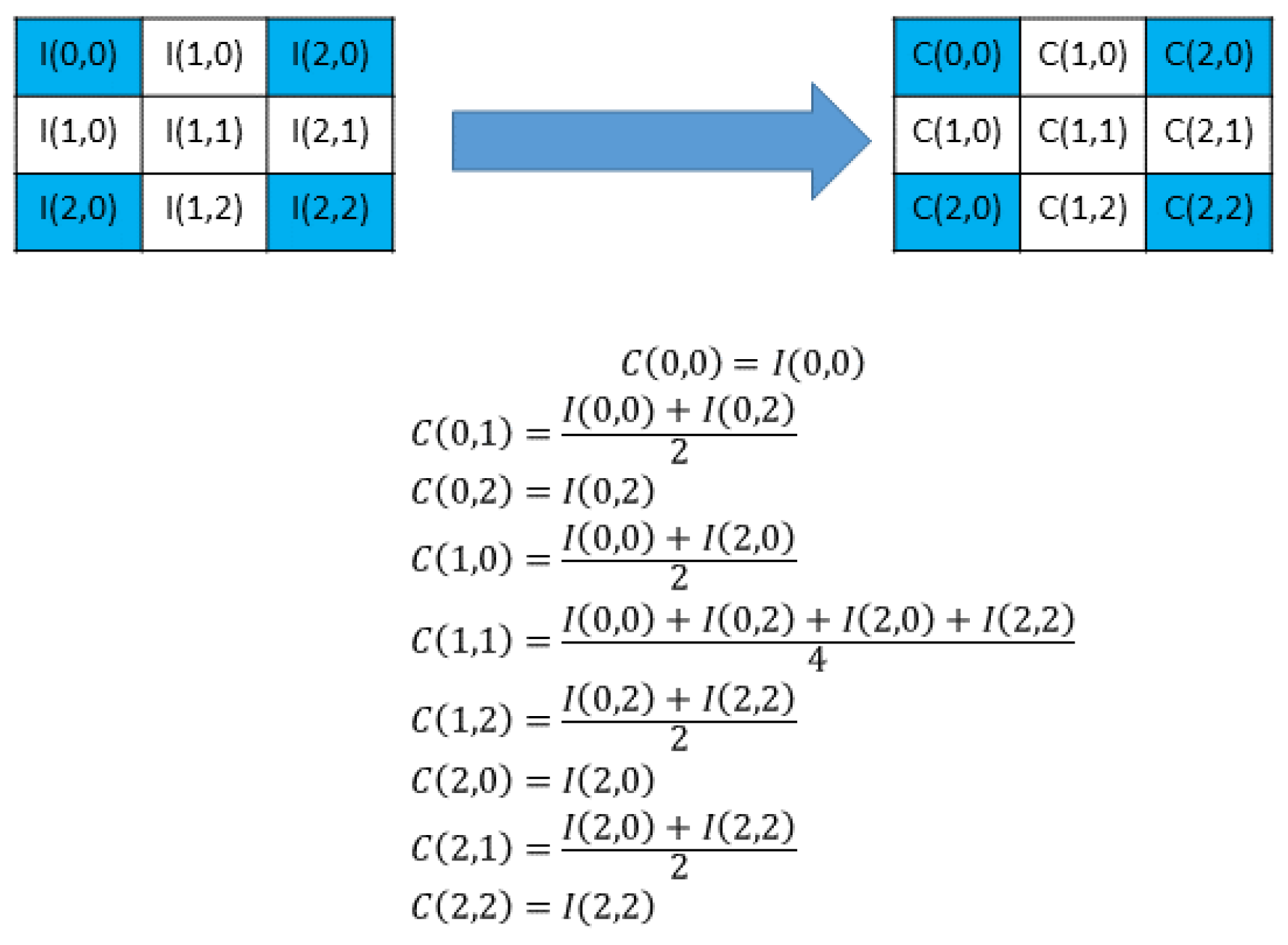
2.3. Enhanced Neighbor Mean Interpolation (ENMI)
To enhance the visual quality of magnified images, Chang et al. [
11] introduced an extension of the interpolation method proposed by Lee and Huang [
12], known as interpolation by neighboring pixels (NMI). Using this approach, the computational procedure for diagonal pixels in NMI was substituted with the average of the four closest original pixels, as depicted in
Figure 2. It is important to emphasize that this modification adheres strictly to the original equation and format. The blue color in
Figure 2 shows the fixed pixels.
2.4. Research Motivation
The previously mentioned techniques, namely, conventional prediction error expansion and pixel-based pixel value ordering predictor, demonstrate proficiency in generating stego images characterized by elevated PSNR values. Nevertheless, these methodologies exhibit shortcomings in terms of security and embedding capacity. A primary deficiency in conventional prediction error expansion lies in its susceptibility to sophisticated attacks. The method is vulnerable to statistical analysis, which may enable adversaries to discern patterns and potentially unveil concealed information.
Conventional prediction error expansion facilitates data concealment within prediction errors; however, its embedding capacity is constrained. The method encounters challenges accommodating larger volumes of data without compromising the quality of the resultant stego content. Such limitations pose practical hindrances in applications necessitating substantial data-hiding capabilities. Analogously, the pixel-based pixel value ordering predictor method faces analogous constraints.
To facilitate the secure transmission of larger volumes of data, we propose a high-payload scheme grounded in interpolation and histogram shifting. In
Section 3, we describe our proposed method.
3. Proposed Method
This section provides a detailed introduction to the proposed method, which is based on enhanced neighbor mean interpolation (ENMI) [
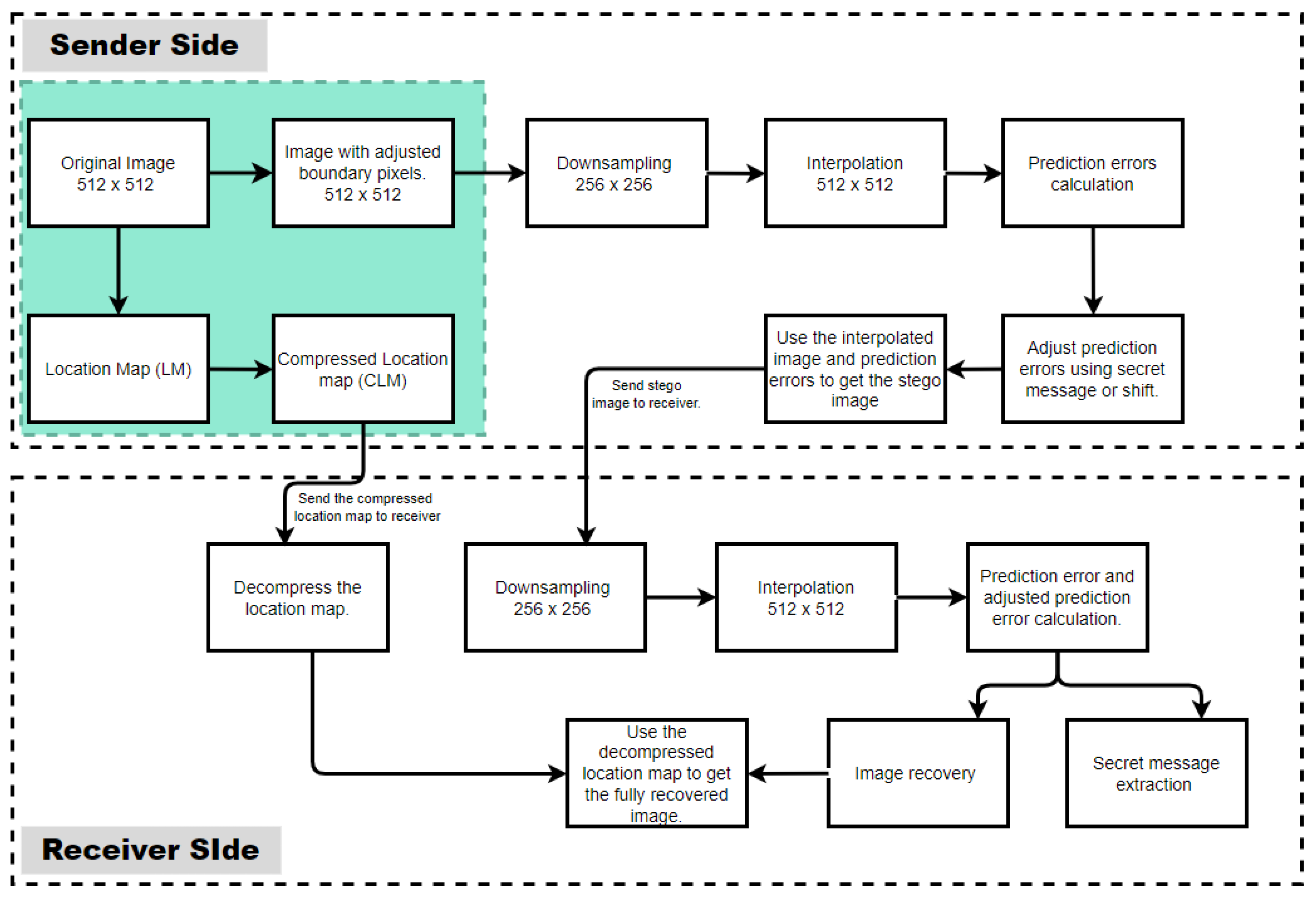
11]. The framework of the proposed method is depicted in
Figure 3. On the sender side, prior to the embedding process, the image boundary pixels are adjusted, and the adjusted pixel locations are recorded in a location map (LM), which is then compressed into a compressed location map (CLM), shown with a blue background in
Figure 3. The image with adjusted boundary pixels is then downsampled. The downsized image with fixed pixel values is used to make an interpolated image. Prediction errors are then calculated. These prediction errors are then adjusted using the secret message (bits) or by shifting. On the receiver side, we first downsample the received stego image and then perform image interpolation. Prediction errors are calculated and adjusted to recover the image and also to extract the secret message. The received compressed location map (LM) is decompressed, the decompressed location map is used to readjust the recovered image, and a fully recovered image is attained. The proposed method was adapted from Chang et al. [
11], although it does not follow the same procedures as ENMI [
11].
3.1. Overflow/Underflow
Prior to delving into a comprehensive discussion of the proposed method, it is imperative to acknowledge that the introduced approach is vulnerable to underflow and overflow at the boundary pixels of 0 and 255. This susceptibility may give rise to minor distortions. The distortion in this method may not be severe, since embedding and shifting are accomplished by −3 and 3, as shall be discussed below. To avoid this situation, the boundary pixels 0 and 255 were changed by 3 units. The grounds for changing by one unit are based on the shifting and embedding being conducted by a three-value unit (3 and −3). As an illustration, 0 has been altered to 3, and 255 has been adjusted to 252. These boundary pixels necessitate preprocessing, after which a location map (LM) is employed to retain pixel information, ensuring pixel reversibility. Utilizing arithmetic coding, the LM can be condensed to generate a compressed location map (CLM).
3.2. Embedding
The embedding process is conducted in a series of steps to obtain the stego image. These steps include downsampling, the interpolation process, calculation of prediction errors, adjustments to prediction errors, and secret embedding and generation of the stego image.
3.2.1. Downsampling
In this step, the image has to be sampled using certain fixed pixel values. The choice of fixed pixel values for utilization during the downsampling process can be executed through various methods, and these methodologies do not impact the performance of the proposed method. For illustration in this method, odd pixel positions were selected as the fixed pixel positions from both the row
R and column
C., i.e.,
where
n is an infinite positive odd number. Please note that both
C and
R must be odd if the pixel position is to be considered as a fixed pixel position. The downsampled pixel is referred to as
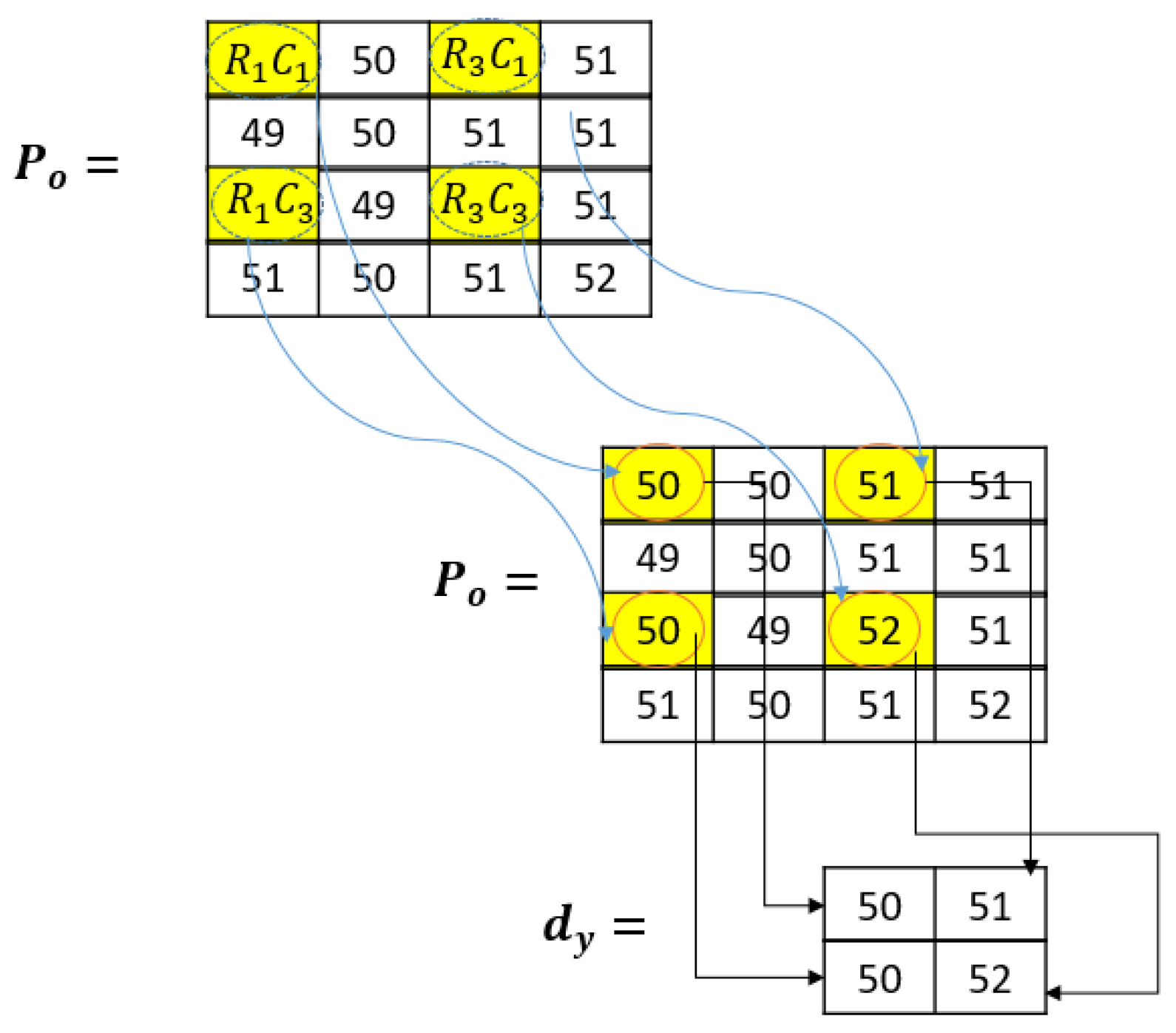
dy. The selected fixed pixel position values are used as the downsampled pixels.
Figure 4 is an example to demonstrate this. The yellow highlight represents the fixed pixel positions while the arrows show these fixed pixel positions which are used during downsampling:
In this example, the downsampling process is demonstrated using four fixed pixels selected through the row and column odd position number system discussed above. Here, R1C1 represents row R = 1 and column C = 1. The same goes for the rest of the highlighted pixel positions. These pixel positions are all from odd positions. Pixel 51 comes from the odd position RC (3,1). The downsampling is shown in the last part of the above image as pixels 50, 51, 50, and 52.
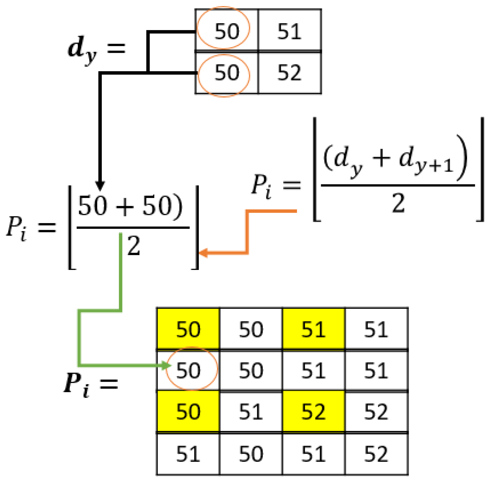
3.2.2. Interpolation
The next step after the downsampling is interpolation. Interpolation generally means fitting data points onto something to represent data. In this method, interpolation refers to fitting pixels to represent the original image pixels and the downsampled pixels. To achieve this, each even pixel point position value is determined by computing the average of two fixed-position pixels from the downsampling. For instance, if the required even position is
RC (1,2), the pixels from
RC (1,1) and
RC (1,3) are averaged and then rounded off to the nearest integer if the average is a floating-point number. The pixel at position
RC (1,2) will have a value equal to this average. This can be carried out using Equation (10).
where
Pi is the interpolated image pixels,
d is the downsampled pixels, and
y is the position of each downsampled pixel in terms of
RC.
Figure 5 is an example of how the interpolated pixels would look given the previous downsampling example:
3.2.3. Prediction Errors
To obtain the prediction errors
Pe, the interpolated pixel values
Pi for each pixel position are subtracted from the corresponding original pixels
Po using Equation (11).
Figure 6 shows an example of this. The yellow highlight marks the fixed pixel positions. The rest of the colors have no significant meaning apart from distinguishing between the original and interpolated pixels.
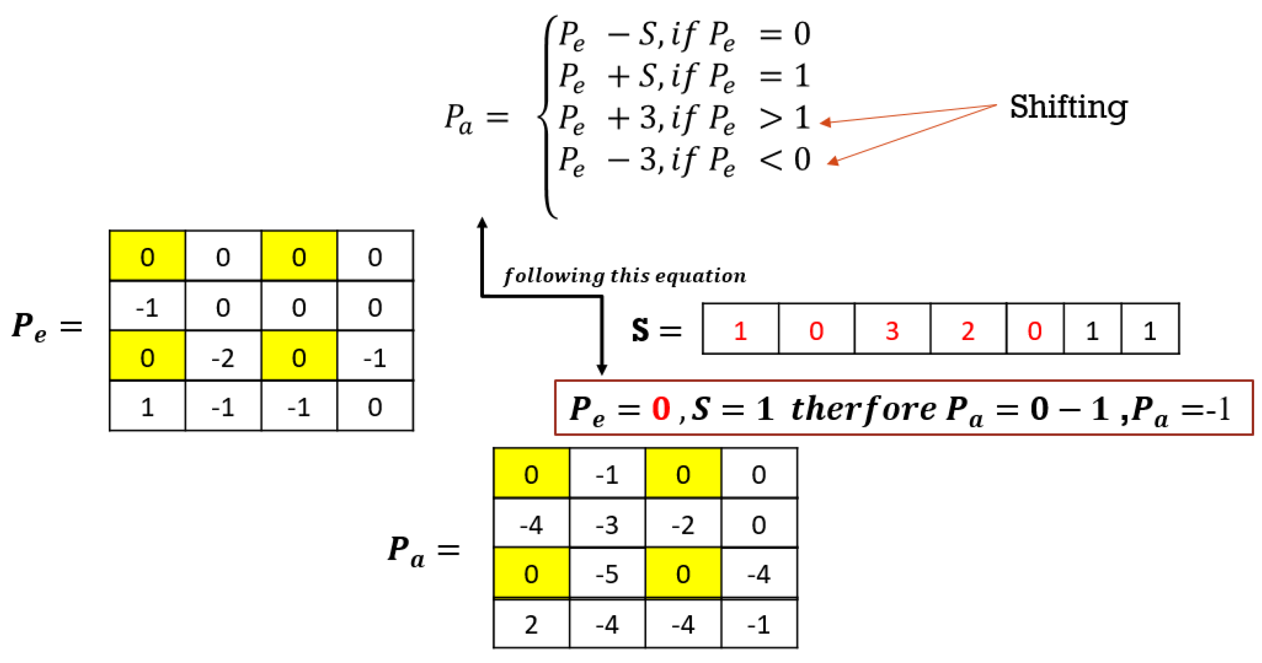
3.2.4. Adjusted Prediction Errors
To embed the secret message
S, adjusted prediction errors
Pa are used. The fixed prediction errors
Pe are not used in the embedding, and as such, they are not adjusted; rather, they are directly copied as adjusted pixel errors
Pa. The rest of the prediction errors are either shifted or used to embed the secret message by subtraction or addition using Equation (12):
where
Pa is the adjusted prediction error,
Pe is the prediction error, and
S is the secret message bit. For this method, shifting is only performed by a maximum of 3 bits during embedding (for
Pe = 1 and
Pe = 0) and normal shifting (for
Pe < 0 and
Pe > 1). This causes some distortion, and, therefore, the PSNR of this method cannot be significantly high. However, it allows for more data to be embedded, hence improving the embedding capacity.
Figure 7 is an example to demonstrate the above explanation. The change in
Pe by +/−3 changes the pixel intensity, subsequently shifting the histogram of the original or stego image. The yellow highlight represents fixed pixel positions while the red font is the secret message to be hidden in the example in
Figure 7.
In
Figure 7, secret message
S is 1011011
2. Using the above equation, the adjusted prediction errors can be found. The fixed pixel positions’ prediction errors will not be adjusted because they are fixed anyways and cannot be used to conceal the secret message. The positions with values less than 0 in the prediction errors
Pe will be shifted left by 1, i.e., −1 will be shifted to −2. The positions with values greater than 1 in the prediction errors
Pe will be shifted right by 1 to obtain the adjusted pixel prediction errors
Pa, i.e., 2 will be shifted to 3. The positions with values equal to 1 in the prediction errors
Pe will embed the secret message by adding the secret message bit to the prediction error
Pe to obtain the adjusted pixel prediction errors, i.e., if the secret bit = 1 and the prediction error = 1, the adjusted pixel errors
Pa will be 2.
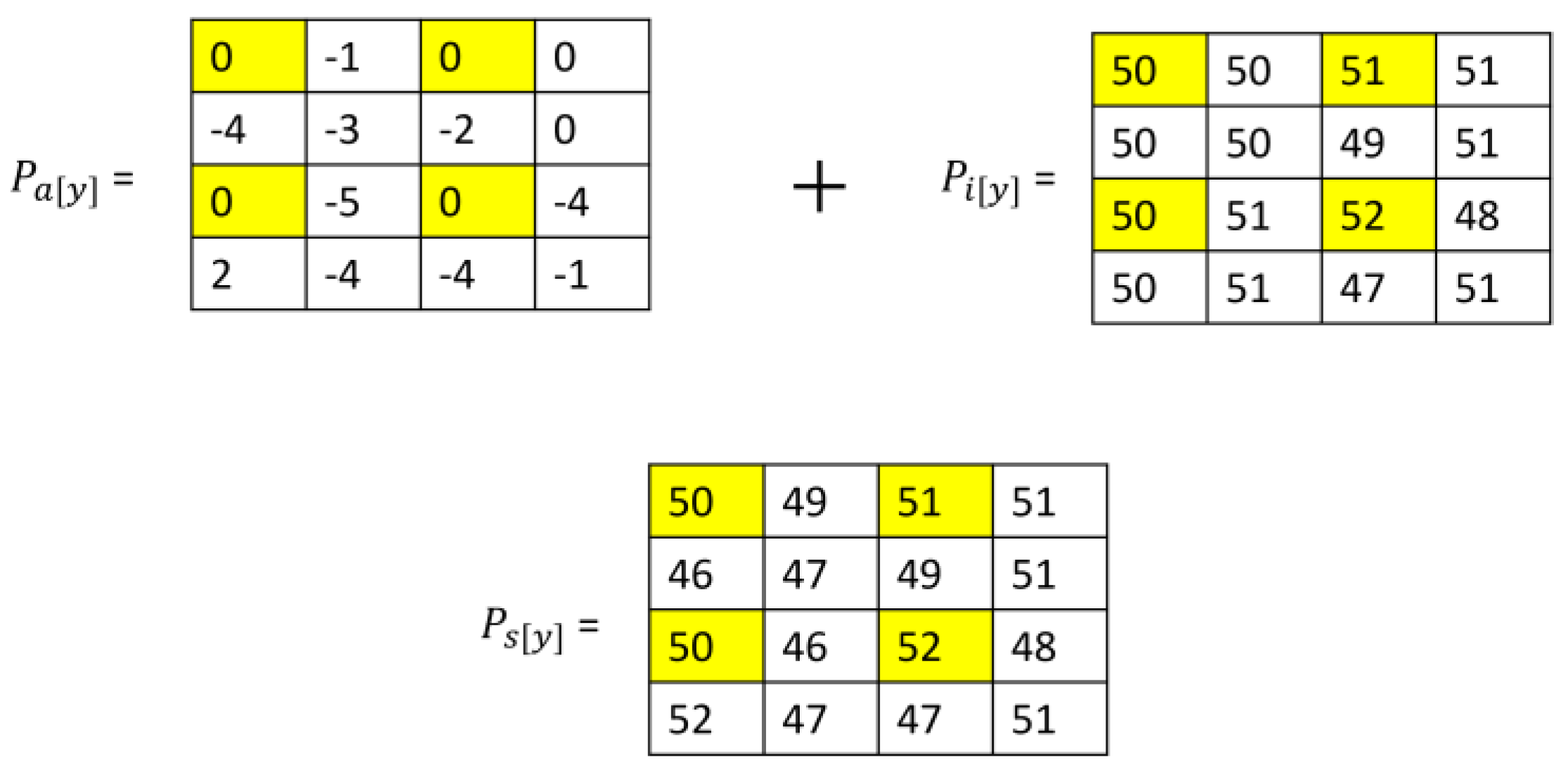
3.2.5. Obtaining the Stego Image
The last stage in the embedding process is obtaining the stego image. To obtain the stego image, the adjusted pixel errors
Pa are added at the corresponding position to the interpolated image pixels
Pi at that position using Equation (13):
where
PS is the stego image pixel and
y is the position of the pixel or prediction errors. For example,
PS [
1] =
Pa [
1] +
Pi [
1].
Figure 8 is an example.
After this step is finished, the embedding process is complete. The sender can send the stego image and the compressed location map (as overhead information) to the receiver through a secure channel.
Figure 8 is an embedding example where the yellow highlights represent the fixed pixel positions.
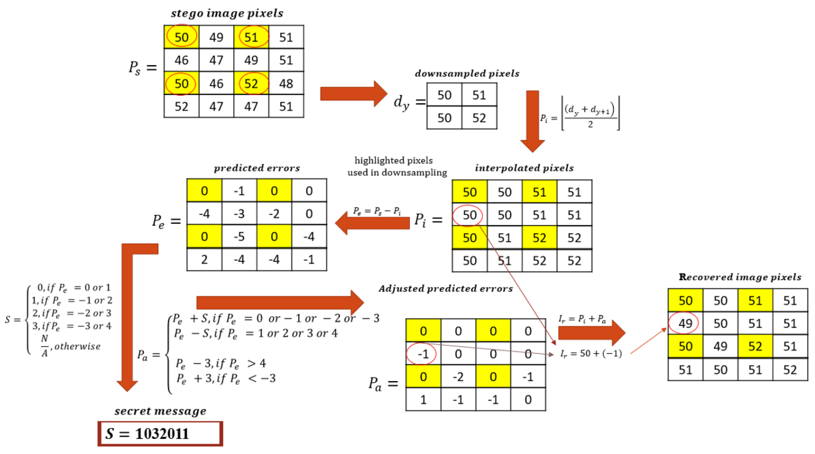
3.3. Extraction and Recovery
Upon receiving the stego image, the receiver has the capability to extract the concealed secrets and restore the image. The extraction and recovery procedures closely mirror the embedding process. The subsequent steps outline the process of secret extraction and image recovery:
3.3.1. Downsampling
Since the stego image’s fixed pixels and the original image’s pixels at the corresponding positions are equal, the same downsampling method can be used as in the extraction process. In this part, just like in the embedding process, the image has to be sampled using certain fixed pixel values. The selection of the fixed pixel values to be used during the downsampling process can be carried out in many different ways; however, the same method that was used for selecting the fixed pixel positions during embedding must be used in selecting the fixed pixel positions during the extraction process, since the fixed pixels are not modified. Following the proposed method of embedding process downsampling, odd pixel positions were selected as the fixed pixel positions from both the row
R and the column
C, using the same equation as in
Section 3.2.1. Please note that both
C and
R must be odd if the pixel position is to be considered as a fixed pixel position. The selected fixed pixel position values are used as the downsampled pixels in the extraction process.
3.3.2. Interpolation
Since downsampling is the same as in the embedding process, the interpolation process in extraction and recovery also follows the same rules and steps as in the embedding process. To accomplish this, each even pixel point position value is found by calculating the average of two fixed position pixels from the downsampling. For instance, if the required even position is RC (1,2), the pixels from RC (1,1) and RC (1,3) are averaged and then rounded off to the nearest integer if the average is a floating-point number. The pixel at position RC (1,2) will have a value equal to this average. The extraction part of interpolation is carried out using Equation (10), as in the interpolation in the embedding process.
3.3.3. Prediction Errors
After interpolation has been completed, the next step is to calculate the prediction errors. To obtain the prediction errors
Pe, the interpolated pixel values
Pi for each pixel position are subtracted from the corresponding stego pixels
Ps using Equation (14):
3.3.4. Adjusted Prediction Errors
To extract the secret message
S, predicted error
Pe equals 0 or 1, with an exception: the fixed positions’ predicted errors will result in an
S value that is equal to 0, while predicted errors with a −1 or 2 value will result in an
S value that is equal to 1. Predicted errors with a −2 or 3 value and predicted errors with a −3 or 4 value will have
S values of 2 and 3, respectively. Other predicted error values apart from those discussed will not have an
S value, which means that there is no secret embedded at that position. To calculate the adjusted prediction errors
Pa, the secret
S is subtracted from the predicted errors
Pe at each corresponding position, with
Pe = 4,
Pe = 3,
Pe = 2, or
Pe = 1. Further, the secret
S is added to the predicted errors
Pe at each corresponding position, with
Pe = 0,
Pe = −1,
Pe = −2, or
Pe = −3. To obtain the adjusted prediction errors for other values, 3 is subtracted from the predicted errors
Pe at each corresponding position with
Pe > 4, and the 3 is added to the predicted errors
Pe at each corresponding position with
Pe < −3. Equations (15) and (16) are used in this calculation:
Finally, to recover the image, the interpolated pixels
Pi are added to the adjusted prediction errors
Pa. The image should be recovered in a lossless fashion. The image recovery is performed using Equation (17):
where
Ir is the recovered image pixel at each position. If any of the boundary pixels were adjusted from the location map, readjust the pixels to obtain the real cover image pixels.
Figure 9 is an example of the whole secret message extraction and recovery process. The pixels with a yellow background are the fixed pixels. The same pixels are marked using a red circle to indicate that they are the pixels selected for down sampling purposes.
3.4. Generic Rivet Cipher 4(RC4 Encrption) Algorithm
The RC4 algorithm, also known as Rivest Cipher 4 or ARC4, is a symmetric stream cipher widely used for encryption in various security protocols. It is known for its simplicity and efficiency. RC4 generates a pseudo-random stream of bits, which is XORed with the plaintext to produce the ciphertext. The algorithm has three main steps: key scheduling, pseudo-random generation algorithm, and encryption.
4. Experimental Results
The experiments for the proposed method were performed using Python 3.7 and Jupiter Notebook, running on a MacBook pro M1 with an Apple m1 chip and an 8GB RAM. For the sake of experimenting with this method, 10 images were adapted from USC-SIPI and used. All images used in the experiment were 512 × 512 pixels in size. The comparison was performed using the embedding capacity, the structural similarity index (SSIM), the peak signal-to-noise ratio (PSNR), and the prediction error histogram. The embedding capacity is a measure of how much data can be embedded into the cover image using the proposed method. In normal cases, a high embedding capacity results in a low PSNR value; however, this is not the case with the proposed method. The proposed method demonstrated a high embedding capacity average of 108,801.1 and an average PSNR value of 40.6 dB when considering the seven images in
Table 1.
The peak signal-to-noise ratio (PSNR) serves as a quantitative metric for comparing images or signals. It is a mathematical equation that articulates the ratio between the power of a signal and the inherent distortion noise that could impact its quality representation. Typically, this expression is conveyed on the logarithmic decibel scale to prevent the representation of excessively large numbers.
In the context of images, the peak signal-to-noise ratio (PSNR) [
13,
14,
15,
16,
17,
18] is commonly employed to assess the distortion introduced in image steganography. A lower PSNR value indicates a more distorted image. For effective steganography algorithms, the PSNR value is expected to exceed 30 dB, as a value beyond this threshold implies that the distortion is imperceptible to the human eye. Additionally, a PSNR value greater than 30 dB is a common benchmark that signifies a good trade-off between the amount of hidden data and the perceptual quality of the stego image. The PSNR value is contingent upon the mean squared error (MSE), as illustrated in Equation (18).
where
MAX is the maximum possible value. In the context of the proposed method, 8-bit grayscale images were employed, and consequently, the
MAX value used was 255. The PSNR equation can be expressed as Equation (19).
The structural similarity index (SSIM) [
17] is utilized for assessing the quality of stego images. A stego image with a value closer to 1 signifies higher image quality. The computation of SSIM can be performed using Equation (20).
where
p,
,
and
q,
,
represent the mean pixel number, variance, and the standard deviation of the original image and stego image, respectively.
is the covariance for the original and stego images. The symbols
and
are constants, where
= k1L and
= k2L. The value of
k1 = 0.01,
k2 = 0.03, and
L is 255 [
19].
The PSNR and SSIM are vital in measuring the performance of the algorithm. Both the structural similarity index (SSIM) and peak signal-to-noise ratio (PSNR) are metrics used to assess the quality of reconstructed signals or images, but they provide different insights. While PSNR focuses on the level of noise or distortion in the signal, SSIM takes into account structural information and human perception. Having both SSIM and PSNR values can offer a more comprehensive evaluation of the quality of a stego image.
Table 1 presents the experimental outcomes for select images utilized in the evaluation of the proposed methodology. The minimum peak signal-to-noise ratio (PSNR) value recorded was 40.1 dB, observed in the case of the baboon image. Conversely, the maximum PSNR value achieved was 40.8 dB. The mean PSNR value for the proposed method, considering the seven images delineated in
Table 1, stood at 40.6 dB. Notably, the proposed method demonstrated an elevated embedding capacity, as evidenced in
Table 1, with an average embedding capacity of 108,801 bits. Across our experiments, the range of embedding capacities varied from a minimum of 39,566 bits to a maximum of 146,170 bits.
Table 1 further demonstrates the SSIM value of the proposed method. As shown, the SSIM values for all the stego images were closer to 1, and therefore, as per the definition and description of the SSIM, the proposed method produced great stego images.
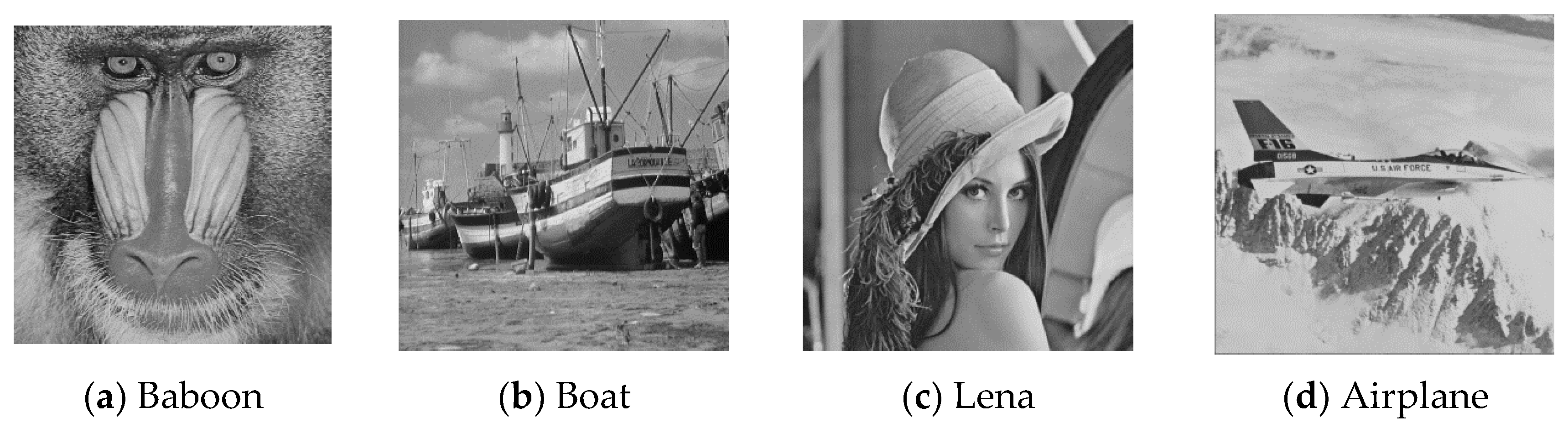
Some of the images (512 × 512) used in our experiments included a baboon, a boat, Lena, and an airplane, and these images are shown in
Figure 10.
Table 2 is a comparison of the proposed method with other methods in terms of the PSNR with an embedding capacity of 10,000 bits. As can be seen, the proposed method could not outperform the other compared methods concerning the PSNR value; however, its PSNR value was above 30 dB, which can be recognized by the human eye. There is usually a trade-off between the embedding capacity and the PSNR. Since the proposed method improved the embedding capacity, it did not perform better than the compared methods with regard to the PSNR.
In the realm of data hiding, the embedding capacity (EC) denotes the quantitative extent to which information can be surreptitiously integrated within a host medium without perceptibly altering its intrinsic attributes. This crucial metric, intrinsic to the discipline of steganography, encapsulates the maximum volume of concealed data that can be seamlessly incorporated while mitigating discernible deviations in the quality or characteristics of the host medium, whether it be an image, audio file, video, or analogous data construct. The pursuit of an optimal embedding capacity resides in the delicate equilibrium between concealing a substantial quantum of information and minimizing any discernible impact, thereby ensuring that the covert alteration remains indiscernible to an observer. This, therefore, means that an increase in the embedding capacity (EC) leads to a decrease in the PSNR value. The embedding capacity, in this context, means the number of bits that can be hidden in the image. The embedding capacity was calculated based on Equation (21).
where
is the number of prediction errors.
Refs. [
13,
14,
15,
16,
20,
21] all describe reversible data-hiding methods in the histogram shifting and/or interpolation domains. All of these methods can produce very high PSNR values and high embedding capacities.
Table 3 shows a comparison of the proposed method with these other previously proposed methods. HPPVO [
13] has an average EC of 37,995 bits, OPPVO [
14] has an average PSNR value of 30,555 bits, IPPVO [
15] has an average EC of 33,723 bits, IPVO [
16] has an average EC value of 32,218 bits, GS-LPVO [
20] has an average EC value of 34,301, and LPVO [
21] has an average EC value of 43,006, while the proposed method has a high EC of 101,283.5 bits. As can be seen, the proposed method has the highest average EC value when compared to these methods; thus, the proposed method is superior to the compared methods with regard to the embedding capacity. The airplane image, which usually has the highest EC in this domain, also shows that the proposed method still has the highest embedding capacity of 146,170 bits, as compared to 51,511 bits from [
16], 60,054 bits from [
15], 53,122 bits from [
14], 62,273 bits from [
13], 49,719 bits from [
20], and 50,129 bits from [
21] using the same image (airplane). The minimum EC that could be produced for all the methods was obtained for the baboon image, for which the proposed method still outperformed the aforementioned ones. The proposed method had an EC of 39 566 bits for this image, as can be seen in
Table 3.
Figure 11 provides a visual representation of the performance of the proposed method at various embedding capacity (EC) values; the graph indicates that the method achieved high peak signal-to-noise ratio (PSNR) values for EC values below 20,000 bits, with a subsequent decline as EC increased. The house image, depicted in green, exhibited a particularly smooth quality, attaining an EC value exceeding 46 dB for EC values below 50,000 bits; however, a further increase in EC led to a 2 dB drop, resulting in a less smooth curve compared to other images.
4.1. Security
Information concealment techniques, such as the one proposed, facilitate the surreptitious transmission of sensitive data within ostensibly innocuous files. This covert methodology poses a formidable challenge for unauthorized entities attempting to detect or intercept the concealed information. A multitude of data-hiding algorithms have been devised across diverse domains, rendering it infeasible for hackers to ascertain the specific method employed for data concealment. Consequently, this complexity deters unauthorized access to the hidden confidential data, thereby fortifying the security of the information. Furthermore, information concealment frequently incorporates encryption, wherein data undergo transformation into an unreadable format without the requisite decryption key. This precaution ensures that, even if unauthorized individuals gain entry to the data, comprehension or utilization remains unattainable without the corresponding decryption key.
In the proposed methodology, for instance, the utilization of the RC4 algorithm can precede the embedding process, contributing to an additional layer of security. Moreover, in data concealment, the stego image typically closely resembles the original image, complicating the ability of hackers to differentiate between an image containing secret data and one that does not. Consequently, it can be asserted that the security of hidden data is substantially elevated. Rigorous assessments are commonly conducted on stego images to validate the algorithm’s resilience against potential attacks. If the algorithm demonstrates robustness in the face of such assessments, the proposed methodology can be deemed secure. One such attack is the rotation attack.
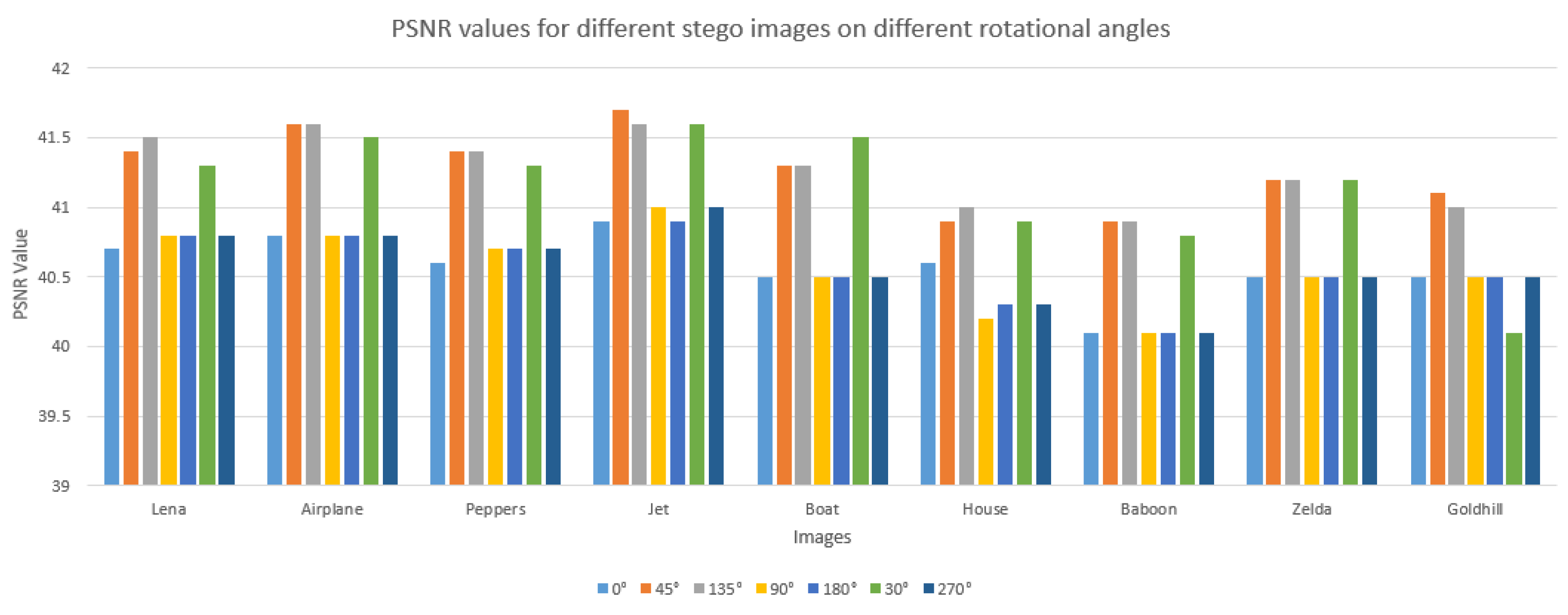
In steganography, a rotation attack [
19] refers to a technique used by adversaries to detect, manipulate, or uncover hidden information within images or other media. This attack involves rotating the carrier medium, typically an image, to reveal patterns or inconsistencies that might indicate the presence of concealed data. Attackers may employ rotation to achieve goals such as detecting hidden information, extracting it, or disrupting it. To counter rotation attacks and enhance steganography security, advanced techniques are used that can withstand rotations and other transformations while maintaining the integrity of the hidden data. Rotations by 0, 45, 135, 90, 180, 30, and 270 degrees were applied to the images. Usually, when a rotation attack can be detected, the PSNR of the images is significantly reduced; however, the proposed method can withstand this kind of attack because the PSNR values produced are not too different from each other as shown in
Figure 12.
4.2. Additional Information
It should be noted that the original binary secret denoted
SLai is first encrypted using RC4 encryption or simple XOR (⊕) to form a new binary secret, denoted as S
Hui. Before the embedding process,
SHui is divided into groups of 2 to create the to-be-embedded secret
S using Equation (22). The final secret after extraction is the decrypted secret
SLai. The implementation of RC4 encryption has not been added to this paper.


