Resilient Electricity Load Forecasting Network with Collective Intelligence Predictor for Smart Cities ^†

Abstract

Accurate electricity forecasting is essential for smart cities to maintain grid stability by allocating resources in advance, ensuring better integration with renewable energies, and lowering operation costs. However, most forecasting models that use machine learning cannot handle the missing values and possess a single point of failure. With rapid technological advancement, smart cities are becoming lucrative targets for cyberattacks to induce packet loss or take down servers offline via distributed denial-of-service attacks, disrupting the forecasting system and inducing missing values in the electricity load data. This paper proposes a collective intelligence predictor, which uses modular three-level forecasting networks to decentralize and strengthen against missing values. Compared to the existing forecasting models, it achieves a coefficient of determination score of 0.98831 with no missing values using the base model in the Level 0 network. As the missing values in the forecasted zone rise to 90% and a single-model forecasting method is no longer effective, it achieves a score of 0.89345 with a meta-model in the Level 1 network to aggregate the results from the base models in Level 0. Finally, as missing values reach 100%, it achieves a score of 0.81445 by reconstructing the forecast from other zones using the meta-model in the Level 2 network.

1. Introduction

With digital technologies becoming more incorporated into smart city management systems, machine learning (ML) is widely proposed as a forecasting model to predict the electricity load with high accuracy in smart cities [1]. Having the capability to accurately forecast the electricity load is necessary to allow the smart grids to distribute the electric power in advance to avoid overloading the electricity delivery network [2], better renewable energy integration with traditional energy to generate electricity [3], and minimize the operation loss during the peak hours [4]. As the scale of electricity infrastructure and reliability directly correlates to economic growth, it is crucial to maintain reliable service to avoid financial losses and interruption of other essential services [5].

However, digitalizing essential infrastructures in smart cities opens up new problems, such as cyberattacks against the infrastructures in smart cities. IBM Security observes this trend where 10.7% of cyberattacks in 2022 happened in the energy sector alone [6]. Looking deeper into distributed denial-of-service (DDoS) attacks that could cause packet loss and bring the server offline [7], the Azure Network Security Team reported that 89% of DDoS attacks span up to one hour [8], which may add missing values (MV) in the electricity load data and disrupt a centralized forecasting system. Due to the importance of energy services, the attack on electricity infrastructure in Ukraine during the Russo–Ukrainian War in 2016 shows the potential weakness of the current system that enemies could exploit [9]. Hence, it is necessary to create a decentralized and resilient forecasting method to solve these issues.

Still, recent studies in forecasting the electricity load showed most ML implementations overlooked the issue posed by MV [10,11], which could occur due to the packet loss and potentially impacting forecasting accuracy in real-world applications. Several methods exist to tackle this problem. Jung et al. [12] proposed a novel imputation technique to fill the MV accurately. In addition, there are also lightweight alternatives that sacrifice accuracy to train and evaluate MLs that use artificial neural networks (ANN), such as padding, which replaces MV with a placeholder value, and masking, which excludes MV from the computation, as noted by Rodenburg et al. [13]. As well as inadequate MV handling, recent studies also disregarded the single point of failure (SPoF) vulnerability, which could bring the entire forecasting system down when the server hosting the centralized ML architecture is offline [14]. Although existing distributed ML architectures could solve this [15], they are inefficient, and the data heterogeneity could negatively impact the accuracy [16].

In this study, we tackle the issues with MV in the electricity load data due to packet loss and SPoF due to the server hosting the forecasting system being taken offline from the DDoS attacks by proposing the Collective Intelligence Predictor (CIP) implementation, forming modular three-level forecasting networks of distributed MLs shown in Figure 1 to forecast the next one hour of electricity load data, matching the DDoS duration. Although weather and calendar data are proven to improve the electricity load forecasting accuracy in existing studies [17,18], this paper focuses solely on the electricity load data to investigate how well the design in CIP could perform against existing methods without relying on external data to negate the accuracy penalty when forecasting with MV.

Each level in CIP represents three forecasting methods that it can use to forecast the electricity load. The modularity comes from CIP behaviors in activating the networks based on the MV percentages in the electricity load data used as independent variables, reducing unnecessary computation to forecast the electricity load. In addition, it increases the effective range the CIP can handle the MV to forecast the electricity load.

During regular operations where the independent variables have no MV, CIP relies exclusively on the base model trained with 0% MV in Level 0 to “predict” the electricity load in the zone CIP was assigned. As there is no MV, the forecasting accuracy from a single base model trained with 0% MV is sufficient to forecast the electricity load accurately. When the MV percentages in the independent variables range from 1% to 90%, CIP uses the meta-model in Level 1 to “improvise” the forecast by combining and refining the predictions from the base models in Level 0. Each base model is trained with different percentages of MV to contribute diversity in handling different MV percentages, allowing a broader effective range of CIP to forecast the electricity load as the MV percentages rise. Finally, when the MV percentages in the independent variables range from 91% to 100%, and it is no longer potent to use Level 1 to forecast, CIP uses the meta-model in Level 2 to create a “copycat” by reconstructing the forecasts taken from other CIPs meta-models in Level 1. Figure 2 summarized the CIP behaviors in activating the networks.

The primary contribution of this paper lies in developing a decentralized multi-level network of MLs that has modularity in its structure, the capability to handle a broader range of MV percentages, and a failsafe mechanism in Level 2 to reconstruct the forecast when handling MV the MV percentages is too high, which is unattainable with existing electricity load forecasting methods. In addition, with the implementation of multiple levels of networks, CIP could reduce unnecessary computation to forecast the electricity load by activating only the necessary MLs to forecast and increase the effective range of MV percentages CIP can handle when needed. Furthermore, CIP uses two feature selections to choose the best electric load data to improve forecasting accuracy and reconstruction. The contributions are significant in pioneering research predicting the electricity load to address security and reliability issues.

After the introduction in Section 1, Section 2 provides the preliminary for the dataset, feature selection algorithms, hyperparameter optimization, network construction, and comparison with the previous studies in this field. Section 3 provides the concept, application, and model training to implement CIP. Section 4 presented the evaluation of CIP with different MV percentages and compared forecasting accuracy with the existing centralized model architectures. Finally, the work is summarized, and we conclude the future planning for this research in Section 5.

2. Related Works

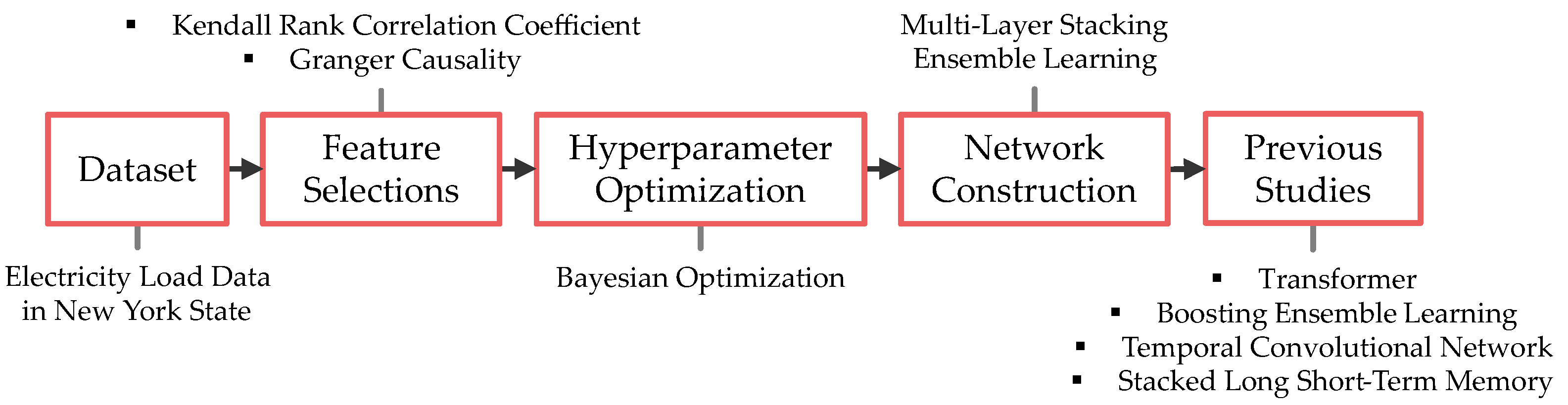
2.1. Overview

This section presents the preliminaries for the dataset, two feature selections to choose the other electricity load zones that may improve the CIP forecasting accuracy or reconstruct the forecast, the hyperparameter optimization algorithm to tune the base model in the Level 0 network of CIP, the multi-layer stacking ensemble learning that the CIP takes the inspiration to construct the networks, and the comparison against the previous studies to forecast the electricity load. Figure 3 shows the high-level summary for the related works implemented to create CIP and compares it against existing methods.

2.2. Dataset

The dataset used to evaluate CIP in this study is publicly available electricity load data sourced from the New York Independent System Operator (NYISO) repository data [19]. It consists of an actual load sampled in real time at 5-minute intervals from 11 zones shown in Figure 4.

The electricity load data taken from the repository to train and evaluate the CIP against existing methods span from 1 January 2018 until 31 December 2020, which is exactly three years, as shown in Figure 5. Once the MV imputed with a polynomial interpolation by order of 2, the training and evaluation datasets split to the ratio 2:1, with the training dataset covering the period from 1 January 2018 to 31 December 2019 and the evaluation dataset from 1 January 2020 to 31 December 2020.

The training dataset normalized from −1 to 1 using the min-max normalization method. Then, using the same minimum and maximum values found in each electricity load zone from the training dataset, the same scale was applied to the evaluation dataset to be normalized for simulating the real-world application, where the latest data are not always used to update the models. After that, sequencing was applied to the datasets to forecast the next hour using the current one hour of electricity load data, which translates to 12 steps in independent and dependent variables. Although the training dataset used a sliding window moving 1 step per sequence to capture intricate patterns, the evaluation data used a sliding window moving 12 steps instead to ease the evaluation. Finally, MV simulated in the independent variables where $MV=\left\{0\%,10\%,20\%,\dots ,90\%\right\}$ to create additional ten independent variables sequences for each zone.

2.3. Feature Selections

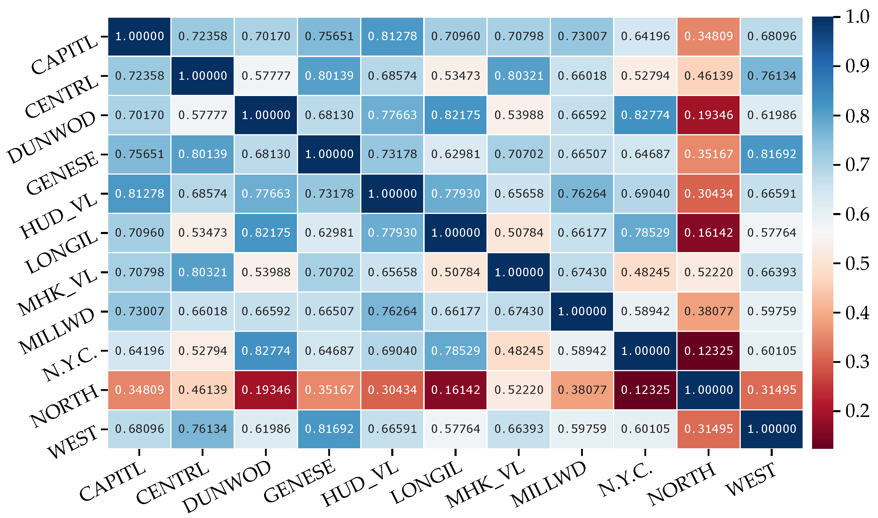
2.3.1. Kendall Rank Correlation Coefficient

CIP utilizes the Kendall rank correlation coefficient in Level 0 and Level 1 networks to find additional electricity load zones that may improve the forecasting accuracy for the electricity load zone CIP will be assigned to forecast.

Kendall rank correlation coefficient measures the strength and direction of the association between two sets of ranked data [20]. Since it is non-parametric, the data distribution does not affect the result [21]. To calculate, find the number of concordant pairs C and discordant pairs D in the ranked data of the training dataset before using Equation (1), where n represents the number of observations.

$$\tau =\frac{C-D}{\frac{1}{2}n\left(n-1\right)},-1\le \tau \le 1$$

(1)

For interpretation, as $\tau$ approaches 1, it indicates a strong positive correlation between two sets of ranked data. Similarly, as $\tau$ approaches $-1$, it indicates a strong negative correlation. However, if $\tau \approx 0$, it indicates weak or no correlation. Using pandas library [22], we compute the correlation for each zone, convert the values into absolute values, and sort it in descending order to choose the zones with high correlation.

2.3.2. Granger Causality

CIP utilizes Granger causality in the Level 2 network to find other electricity load zones that may improve the reconstruction of the forecast in the zone where the MV percentage is 91% and above. The motives for using a different feature selection in Level 2 are to avoid selecting the matching zones in the Kendall rank correlation coefficient to ensure redundancy and, as Granger causality is better in reconstructing the forecast.

Granger causality is a statistical hypothesis test to evaluate if a time series $y_t$ possesses causality for another time series $x_t$ [23]. With “var” represents the variance of a random variable, ${\mathcal{H}}_{<t}$ as the history of all relevant information up to $t-1$ and $\mathcal{P}\left(x_t|{\mathcal{H}}_{<t}\right)$ as the optimal prediction for $x_t$ given ${\mathcal{H}}_{<t}$, y is causal to x if it met the condition shown in Equation (2). As we want to analyze the causality with the time lag from 1 to 6, Equation (2) was rewritten as Equation (3) to reflect this change.

$$\mathrm{var}\left[x_t-\mathcal{P}\left(x_t|{\mathcal{H}}_{<t}\right)\right]<\mathrm{var}\left[x_t-\mathcal{P}\left(x_t|{\mathcal{H}}_{<t}\setminus y_{<t}\right)\right]$$

(2)

$$\mathrm{var}\left[x_t-\mathcal{P}\left(x_t|{\mathcal{H}}_{<t}\right)\right]<\mathrm{var}\left[x_t-\mathcal{P}\left(x_t|{\mathcal{H}}_{<t}\setminus \left\{y_{t-1},y_{t-2},y_{t-3},\dots y_{t-6}\right\}\right)\right]$$

(3)

After calculating the differences between consecutive observations in the dataset two times, we perform the Granger causality tests using statsmodels library [24] to obtain the p-values, which we sort in ascending order to find zones with high causality.

2.4. Hyperparameter Optimization

One of the challenges in designing the CIP is to tune the hyperparameters for the base model in Level 0, as there is no single best set of hyperparameters due to the complex relationships between them, requiring trial and error to find the best combination [25]. CIP utilizes Bayesian optimization as it utilizes new parameter combinations and exploits known promising regions to navigate the optimization space efficiently [26], which could shorten the computation time and guarantee an optimized outcome. With A as the search space of z, Equation (4) describes the optimization goal to find the maximum value at the sampling point of an unknown function f.

$$z^{+}=\arg {\max }_{z\in A}f\left(z\right)$$

(4)

We use Keras Tuner library [27] to implement the Bayesian optimization to optimize the hyperparameters in the base model, as it has good integration and ease of application with the TensorFlow library [28] used to build the ML models in CIP.

2.5. Network Construction

CIP takes inspiration to construct the networks from the multi-layer stacking ensemble learning. Stacking ensemble learning is a methodology to combine heterogenous base models to create a superior model compared to its components [29]. Compared to other ensemble techniques that use a deterministic way to combine the base models, stacking ensemble learning relies on a non-deterministic algorithm to combine the base models with a meta-model. Figure 6 shows the implementation example of a multi-layer stacking ensemble learning to forecast the electricity load in zone $\alpha$. A set of i base models that use different algorithms are implemented in Level 0 to add diversity in capturing different patterns in zone $\alpha$. In Level 1, a set of j meta-models combines the forecasting outcomes from the base models in Level 0 to improve the accuracy. In Level 2, a final meta-model refines the forecasts further by combining the output from the meta-models in Level 1. Most multi-layer stacking ensemble learning is limited to three layers, as the accuracy improvement greatly diminishes when adding a new layer.

However, CIP does not fully adhere to the conventional method of deploying multi-layer stacking ensemble learning. Instead of using heterogeneous base models that use different algorithms in each base model, the base models in CIP are homogeneous, where the diversity in handling different percentages of MV is from training each base model with various percentages of MV. In addition, the independent variables are exposed to the meta-models in Level 1 and Level 2 networks to help the meta-models grasp the amount of MV they need to consider when combining the forecasts. Finally, the meta-model in the Level 2 network uses the forecasting outcomes taken from other CIPs Level 1 networks to reconstruct the prediction. Section 3.2 will discuss more in detail on CIP network implementation.

2.6. Previous Studies

The most commonly used models to forecast the electricity load rely on the Recurrent Neural Networks (RNN)-based implementation and its derivatives, such as long short-term memory (LSTM) and Gated Recurrent Unit (GRU), due to their capability to capture long-term dependencies in sequential data with high accuracy [30]. In addition, the advancement of technologies and techniques in ANN brings new model architectures that show promising results in forecasting the electricity load. For example, forecasting models that rely on temporal convolutional network architecture (TCN) can capture the local dependencies in the data via convolutional layers, which contributes to shorter interfacing time when compared to the RNN-based derivatives [31,32]. As well as TCN, forecasting models that rely on Transformer architecture show parallelization capabilities when compared to the RNN-based derivatives with the implementation of attention mechanism to capture the relationships between the elements in the sequential data [33,34]. However, they share issues mentioned in Section 1, where the forecasting models that rely on RNN-based derivatives, TCN, and Transformer cannot directly handle the MV due to packet loss from the DDoS attack without relying on some form of imputation, masking, and padding.

As well as relying on masking, padding, or imputation to make existing models capable of handling MV, several forecasting model designs could directly handle the MV. Stratigakos et al. [35] proposed handling the MV with Linear Programming (LP) to formulate a robust regression model that minimizes the worst-case loss when a subset of the independent variables has MV. The authors noted that their method can handle up to 50% of MV. In addition, Mienye et al. [36] found that an ensemble learning that utilizes boosting is effective when handing MV. Grotmol et al. [37] expand further using stacking ensemble learning that implemented boosting and other ML models as the base models to harden against MV. The authors noted that using heterogeneous base models in stacking could improve the Mean Absolute Error (MAE) score by 10.7%. Although these methods could effectively reduce the accuracy penalty when forecasting with MV, the centralized ML architectures make them suffer from SPoF vulnerability due to the server hosting the forecasting system being taken offline from the DDoS attacks.

Although several distributed computing methods could solve the SPoF vulnerability when the server hosting the forecasting system is taken offline by the DDoS attacks, recent studies show that federated learning is the favorable method due to the capability to train the model in independent sessions without sharing the datasets that may contain sensitive information [38,39,40]. However, in addition to the inefficiency and data heterogeneity negatively impacting the accuracy mentioned in Section 1, the studies in federated learning did not consider the countermeasures against MV.

We previously developed multivariate models to create a distributed forecasting network. Using the electricity load data from the zones with high Kendall rank correlation coefficient values negates the accuracy penalty when using padding to replace MV. In addition, it can substitute the forecast from an offline model by averaging the predictions from other models. However, as the models trained with only 25% of MV in the dataset to avoid overfitting where the models exhibit behaviors where the accuracy will only improve as the MV percentages rise, the effective range it could perform well before the coefficient of determination ($r^2$) score dropped below $0.95$ is limited to 40% of MV. Furthermore, the network does not fully solve the SPoF vulnerability, as it does not have the countermeasure when one of the nodes supplying the electricity loads is offline.

Table 1. Comparison between previous studies to forecast the electricity load and their capabilities to handle missing values and the single point of failure.

Methodology	Missing Values	Single Point of Failure
Robust Model [35]	✓	×
Transformer [33,34]	△	×
Forecasting Network	✓	△
Federated Learning [38,39,40]	×	✓
Boosting Ensemble Learning [36,37]	✓	×
Temporal Convolutional Network [31,32]	△	×
Recurrent Neural Network Derivatives [30]	△	×

✓ = good, △ = moderate, × = bad.

summarized the previous studies and their capabilities in handling MV and SPoF.

In this study, we compare CIP against four existing electricity load forecasting models shown in the list below:

• TCN + padding
• Transformer + padding
• Stacked LSTM + padding
• Boosting ensemble learning

We use padding to help some existing models forecast with MV, as masking may change the sequence length during computation, negatively affecting the forecasting model to capture the dependencies in sequential data. In addition, without imputation to augment the sequence, we can analyze the strength of each model in handling MV.

3. Implementation

3.1. Overview

This section presents the CIP concept to implement modular three-level forecasting networks, its application on feature selections, hyperparameter optimization, and network construction to forecast the electricity load in zone $WEST$ of New York State, and the training methods used to train the ML models in Level 0, Level 1, and Level 2 networks in CIP. Figure 7 shows the high-level summary for the CIP concept, implementation, and training to implement CIP.

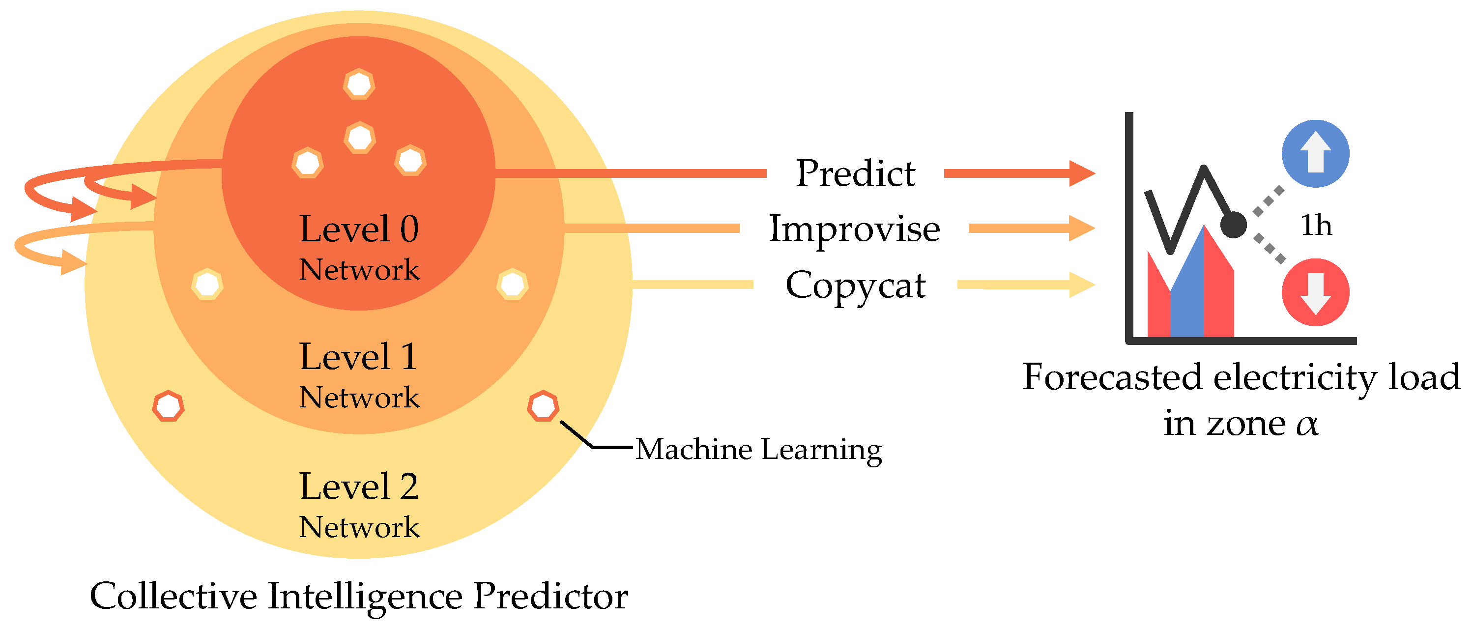
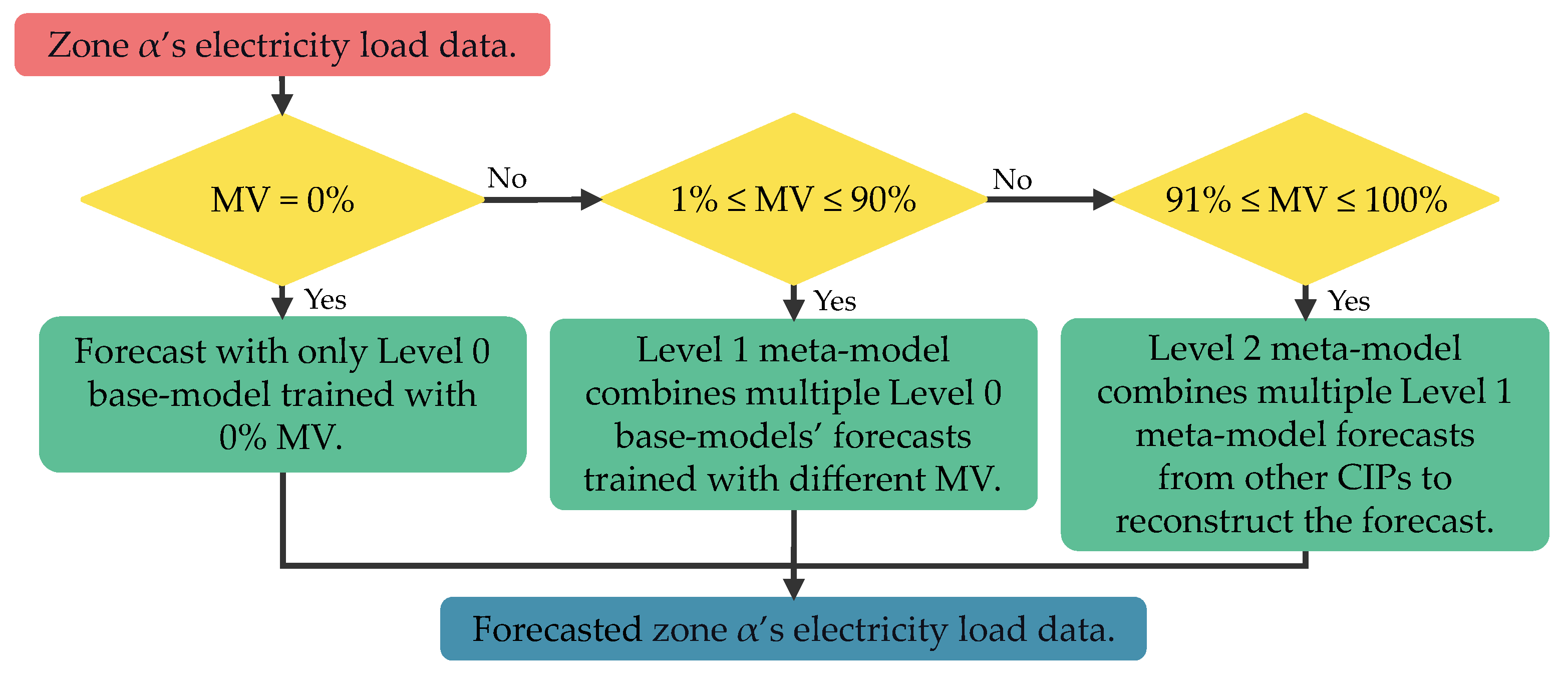
3.2. Concept

Referring to the generalized overview of CIP in Figure 1, CIP utilizes multi-level networks to distribute the ML models as a countermeasure against SPoF vulnerability. The models are connected to form forecasting networks similar to the multi-layer stacking ensemble learning, shown in Figure 6 to reduce the accuracy penalty when forecasting with MV. Figure 8 represented the CIP networks architecture to forecast the electricity load in zone $\alpha$, where we define the $CI{P}_{\alpha }$’s forecast using the “predict” method as $\widehat{{\alpha }_{Predic{t}_{12\le t<24}}}$, “improvise” method as $\widehat{{\alpha }_{Improvis{e}_{12\le t<24}}}$, and “copycat” method as $\widehat{{\alpha }_{Copyca{t}_{12\le t<24}}}$.

Referring to the summarized CIP behavior in Figure 2, CIP has a hierarchical network structure of Level 0, Level 1, and Level 2 to handle different MV percentages accordingly. With Predict(), Improvise(), and Copycat() functions representing “predict,” “improvise,” and “copycat” forecasting methods in $CI{P}_{\alpha }$, Algorithm 1 shows the pseudocode to choose either “predict”, “improvise”, or “copycat” forecasting method based on the total MV percentage in the independent variables (${\alpha }_{0\le t<12}$, ${\beta }_{0\le t<12}$, ${\gamma }_{0\le t<12}$).

Algorithm 1 Networks activation in $CI{P}_{\alpha }$.

Input: ${\alpha }_{0\le t<12},{\beta }_{0\le t<12},{\gamma }_{0\le t<12}$ Output: $\widehat{{\alpha }_{12\le t<24}}\in \left\{\widehat{{\alpha }_{Predic{t}_{12\le t<24}}},\widehat{{\alpha }_{Improvis{e}_{12\le t<24}}},\widehat{{\alpha }_{Copyca{t}_{12\le t<24}}}\right\}$   1: $concatenate\leftarrow {\alpha }_{0\le t<12}+{\beta }_{0\le t<12}+{\gamma }_{0\le t<12}$   2: $mv\_count\leftarrow \left|\{c_i\in concatenate:c_i=\mathrm{null}\}\right|$   3: $mv\_percentage\leftarrow mv\_count/\left|concatenate\right|\times 100\%$   4: if $mv\_percentage=0$ then   5:     $\widehat{{\alpha }_{Predic{t}_{12\le t<24}}}\leftarrow \mathrm{Predict}\left(\right)$   6:     return $\widehat{{\alpha }_{Predic{t}_{12\le t<24}}}$   7: else if $1\le mv\_percentage\le 90$ then   8:     $\widehat{{\alpha }_{Improvis{e}_{12\le t<24}}}\leftarrow \mathrm{Improvise}\left(\right)$   9:     return $\widehat{{\alpha }_{Improvis{e}_{12\le t<24}}}$ 10: else if $91\le mv\_percentage\le 100$ then 11:     $\widehat{{\alpha }_{Copyca{t}_{12\le t<24}}}\leftarrow \mathrm{Copycat}\left(\right)$ 12:     return $\widehat{{\alpha }_{Copyca{t}_{12\le t<24}}}$ 13: end if

3.2.1. Level 0

When the sum of MV percentages in the independent variables is 0%, CIP relies on the “predict” forecasting method in Level 0, where CIP uses only the $Bas{e}_{0{\%}_{\alpha }}$ base model in Level 0 to obtain $\widehat{{\alpha }_{Predic{t}_{12\le t<24}}}$, reducing unnecessary computation and operation cost in regular operation to forecast the electricity load during normal operation. The only time CIP will activate all the base models in Level 0 is when the MV percentages in the independent variables are more than 1%, as the meta-model in Level 1 needs to combine the forecasts from the base models to obtain $\widehat{{\alpha }_{Improvis{e}_{12\le t<24}}}$.

CIP uses ten base models $Bas{e}_{M{V}_{\alpha }}$ in $CI{P}_{\alpha }$ trained using the dataset simulated with MV in Section 2.2 to introduce diversity in handling a wide range of MV percentages during deployment. The base-model architecture shown in Figure 9 is a multivariable stacked LSTM that utilizes hyperbolic tangent (TanH) as the activation function in each layer, where k and l represent the number of LSTM units in the first and second layers of the base-model.

Assuming the electricity load zones from $\beta$ and $\gamma$ could improve the electricity load forecast in zone $\alpha$, we choose multivariable stacked LSTM as the architecture in the base model due to its capability to grasp the dependencies from the independent variable CIP wants to forecast (${\alpha }_{0\le t<12}$) and independent variables that have strong correlation to improve the forecasting accuracy (${\beta }_{0\le t<12},{\gamma }_{0\le t<12}$) in zone $\alpha$, allowing each of the base model in Level 0 to have a broader range of MV percentages it can handle before the forecasting accuracy degrade.

With $Bas{e}_{0{\%}_{\alpha }}$$\left(\right)$ representing the base model trained with dataset that has 0% of MV, Algorithm 2 shows the pseudocode for Predict() function to obtain $\widehat{{\alpha }_{Predic{t}_{12\le t<24}}}$.

Algorithm 2 Predict() function in $CI{P}_{\alpha }$.

Input: ${\alpha }_{0\le t<12},{\beta }_{0\le t<12},{\gamma }_{0\le t<12}$ Output: $\widehat{{\alpha }_{Predic{t}_{12\le t<24}}}$   1: $\widehat{{\alpha }_{Predic{t}_{12\le t<24}}}\leftarrow Bas{e}_{0{\%}_{\alpha }}({\alpha }_{0\le t<12},{\beta }_{0\le t<12},{\gamma }_{0\le t<12})$   2: return $\widehat{{\alpha }_{Predic{t}_{12\le t<24}}}$

3.2.2. Level 1

When the MV percentages in the independent variables ranged from 1% to 90%, CIP relies on the “improvise” forecasting method in Level 1, where all $Bas{e}_{M{V}_{\alpha }}$ in $CI{P}_{\alpha }$’s Level 0 are activated for the $Met{a}_{{\alpha }_1}$ meta-model in Level 1 to combine their forecasts. As each $Bas{e}_{M{V}_{\alpha }}$ has its effective MV percentage range to forecast the electricity load, combining the result with $Met{a}_{{\alpha }_1}$ ensures minimal forecasting accuracy degradation as the MV percentage rises, which is impossible with the bagging ensemble learning that averages the forecasts from the base models.

Following the same assumption in Level 0, CIP combine the forecasts from all $Bas{e}_{M{V}_{\alpha }}$ in Level 0 ($\widehat{{\alpha }_{Base\_0{\%}_{12\le t<24}}},\widehat{{\alpha }_{Base\_10{\%}_{12\le t<24}}},\widehat{{\alpha }_{Base\_20{\%}_{12\le t<24}}},\dots ,\widehat{{\alpha }_{Base\_90{\%}_{12\le t<24}}}$) and the same electricity load data (${\alpha }_{0\le t<12},{\beta }_{0\le t<12},{\gamma }_{0\le t<12}$) used by $Bas{e}_{M{V}_{\alpha }}$ using $Met{a}_{{\alpha }_1}$. The meta-model architecture shown in Figure 10 uses a multivariable deep neural network (DNN) model that utilizes TanH as the activation function in each dense layer. The numbers 156, 75, and 75 represent the dense unit numbers in the first, second, and third layers of $Met{a}_{{\alpha }_1}$. We choose multivariable DNN as the architecture in the meta-model due to its capability to fine-tune the combined forecasts from the $Bas{e}_{M{V}_{\alpha }}$ by the amount of MV that exists in the electricity load data used to forecast in zone $\alpha$, which is impossible with other algorithms that do not consider the amount of MV in the independent variables.

With $Met{a}_{{\alpha }_1}\left(\right)$ function representing the multivariable DNN meta-model in Level 1 network, Algorithm 3 shows the pseudocode to concatenate the forecasts from all $Bas{e}_{M{V}_{\alpha }}$ and the electricity load data used by $Bas{e}_{M{V}_{\alpha }}$ to obtain $\widehat{{\alpha }_{Improvis{e}_{12\le t<24}}}$.

Algorithm 3 Improvise() function in $CI{P}_{\alpha }$.

Input: ${\alpha }_{0\le t<12},{\beta }_{0\le t<12},{\gamma }_{0\le t<12}$        and $\widehat{{\alpha }_{Base\_0{\%}_{12\le t<24}}},\widehat{{\alpha }_{Base\_10{\%}_{12\le t<24}}},\widehat{{\alpha }_{Base\_20{\%}_{12\le t<24}}},\dots ,\widehat{{\alpha }_{Base\_90{\%}_{12\le t<24}}}$ Output: $\widehat{{\alpha }_{Improvis{e}_{12\le t<24}}}$   1: $concat\_a\leftarrow {\alpha }_{0\le t<12}+{\beta }_{0\le t<12}+{\gamma }_{0\le t<12}$   2: $concat\_b\leftarrow \widehat{{\alpha }_{Base\_0{\%}_{12\le t<24}}}+\widehat{{\alpha }_{Base\_10{\%}_{12\le t<24}}}+\widehat{{\alpha }_{Base\_20{\%}_{12\le t<24}}}+\dots +\widehat{{\alpha }_{Base\_90{\%}_{12\le t<24}}}$   3: $concat\_c\leftarrow concat\_a+concat\_b$   4: $\widehat{{\alpha }_{Improvis{e}_{12\le t<24}}}\leftarrow Met{a}_{{\alpha }_1}(concat\_c)$   5: return $\widehat{{\alpha }_{Improvis{e}_{12\le t<24}}}$

3.2.3. Level 2

When the MV percentages in the independent variables exceed 90%, CIP relies on the “copycat” forecasting method in Level 2, where $Met{a}_{{\alpha }_2}$ in Level 2 reconstruct the forecasts in zone $\alpha$ by combining the forecast from the $Met{a}_1$ meta-models in Level 1 taken from $CI{P}_{\beta }$, $CI{P}_{\gamma }$, and $CI{P}_{\delta }$. Although it is inferior in accuracy, it performs well in high MV environments where “predict” and “improvise” failed.

Similar to the $Met{a}_{{\alpha }_1}$ in Level 1, the meta-model $Met{a}_{{\alpha }_2}$ shown in Figure 11 uses a multivariable DNN model that utilizes TanH as the activation function in each dense layer. The only differences are the number of dense units in the first, second, third, and fourth layers, which are 144, 144, 72, and 36. With the assumption that electricity load zones $\beta$, $\gamma$, and $\delta$ could reconstruct the electricity load forecast in zone $\alpha$, $Met{a}_{2_{\alpha }}$ combines the forecasts with strong causality taken from the $Met{a}_1$ in Level 1 of $CI{P}_{\beta }$, $CI{P}_{\gamma }$, and $CI{P}_{\delta }$ ($\widehat{{\beta }_{Improvis{e}_{12\le t<24}}},\widehat{{\gamma }_{Improvis{e}_{12\le t<24}}},\widehat{{\delta }_{Improvis{e}_{12\le t<24}}}$) together with the electricity load data corresponding to the zones other CIPs are assigned (${\beta }_{0\le t<12},{\gamma }_{0\le t<12},{\delta }_{0\le t<12}$) to reconstruct the electricity load forecast in zone $\alpha$ as $\widehat{{\alpha }_{Copyca{t}_{12\le t<24}}}$. As redundancy is necessary for reconstruction, $Met{a}_{2_{\alpha }}$ uses Granger causality to avoid selecting the same data chosen by the Kendall rank correlation coefficient used in Level 0 and Level 1 networks.

With $Met{a}_{2_{\alpha }}\left(\right)$ function representing the multivariable DNN meta-model in Level 2 network, Algorithm 4 shows the pseudocode to concatenate the electricity load data and the forecasts from the $Met{a}_1$ in Level 1 in $CI{P}_{\beta }$, $CI{P}_{\gamma }$, and $CI{P}_{\delta }$ to obtain $\widehat{{\alpha }_{Copyca{t}_{12\le t<24}}}$.

Algorithm 4 Copycat() function in $CI{P}_{\alpha }$.

Input: ${\beta }_{0\le t<12},{\gamma }_{0\le t<12},{\delta }_{0\le t<12}$        and $\widehat{{\beta }_{Meta\_1_{12\le t<24}}},\widehat{{\gamma }_{Meta\_1_{12\le t<24}}},\widehat{{\delta }_{Meta\_1_{12\le t<24}}}$ Output: $\widehat{{\alpha }_{Improvis{e}_{12\le t<24}}}$   1: $concat\_a\leftarrow {\beta }_{0\le t<12}+{\gamma }_{0\le t<12}+{\delta }_{0\le t<12}$   2: $concat\_b\leftarrow \widehat{{\beta }_{Meta\_1_{12\le t<24}}}+\widehat{{\gamma }_{Meta\_1_{12\le t<24}}}+\widehat{{\delta }_{Meta\_1_{12\le t<24}}}$   3: $concat\_c\leftarrow concat\_a+concat\_b$   4: $\widehat{{\alpha }_{Copyca{t}_{12\le t<24}}}\leftarrow Met{a}_{2_{\alpha }}(concat\_c)$   5: return$\widehat{{\alpha }_{Copyca{t}_{12\le t<24}}}$

3.3. Application

3.3.1. Feature Selections

In this study, $CI{P}_{WEST}$ was implemented to forecast the electricity load in zone $WEST$ of the New York State. To construct the Level 0, Level 1, and Level 2 networks in $CI{P}_{WEST}$, Kendall rank correlation coefficient and Granger causality introduced in Section 2.3 used on the training dataset prepared in Section 2.2 with 0% of MV. Figure A1 and Figure A2 shown in Appendix A are the generated feature selection heatmap on the training dataset. Using the Kendall rank correlation coefficient, zones $GENESE$ and $CENTRL$ are used to construct the Level 0 and Level 1 networks in $CI{P}_{WEST}$. Using Granger causality, zones $GENESE$, $NORTH$, and $MHKVL$ are suggested to construct Level 2 network in $CI{P}_{WEST}$. However, as the Kendall rank correlation coefficient has selected $GENESE$, we replace it with $NORTH$ as the next zone with high causality to ensure redundancy.

Figure 12 shows the $CI{P}_{WEST}$ network implementation based on the zones selected by Kendall rank correlation coefficient and Granger causality to construct the Level 0, Level 1, and Level 2 networks. As the $Met{a}_{2_{WEST}}$ in $CI{P}_{WEST}$ requires the $Met{a}_1$ forecasts taken from $CI{P}_{NORTH}$, $CI{P}_{MHKVL}$, and $CI{P}_{CAPITL}$, we implemented the CIPs up to Level 1 network, where the selected zones for each CIP network shown in

Table 2. The zones selected by Kendall rank correlation coefficient to create the Level 0 and Level 1 networks in $CI{P}_{NORTH}$, $CI{P}_{MHKVL}$, and $CI{P}_{CAPITL}$.

Forecaster	Required Independent Variable	Selected Independent Variables
$CI{P}_{NORTH}$	$NORTH$	$MHKVL$, $CENTRL$
$CI{P}_{MHKVL}$	$MHKVL$	$CENTRL$, $CAPITL$
$CI{P}_{CAPITL}$	$CAPITL$	$HUDVL$, $GENESE$

.

3.3.2. Hyperparameter Optimization

Using the Keras Tuner introduced in Section 2.4, we optimized the hyperparameters for the base models implemented in $CI{P}_{WEST}$, $CI{P}_{NORTH}$, $CI{P}_{MHKVL}$, and $CI{P}_{CAPITL}$ with Bayesian optimization. Using fixed randomization, we tuned the base models using the training dataset with 0% of MV prepared in Section 2.2, optimization objective set to minimize the root-mean-square error (RMSE) score, five initial random points to start, and a maximum number of trials set to 5. Furthermore, we set the search range for the first and second LSTM layers units from 32 to 256 with 32 steps and the learning rate for Adam to choose from 0.001, 0.0001, and 0.00001.

Table 3. The hyperparameters obtained for the base models in $CI{P}_{WEST}$, $CI{P}_{NORTH}$, $CI{P}_{MHKVL}$, and $CI{P}_{CAPITL}$ with Bayesian optimization.

Base Model	First LSTM Layer Units	Second LSTM Layer Units	Adam’s Learning Rate
$CI{P}_{WEST}$	192	96	0.001
$CI{P}_{NORTH}$	128	128	0.001
$CI{P}_{MHKVL}$	192	96	0.001
$CI{P}_{CAPITL}$	192	96	0.001

shows the hyperparameter optimization outcome. Most base models share the same hyperparameters, except the base model in $CI{P}_{NORTH}$. Most likely, it is due to most zones having a weak correlation zone $North$, leading to a different optimization outcome.

3.4. Training

3.4.1. Level 0

To train the $Bas{e}_{M{V}_{WEST}}$ in the Level 0 network of $CI{P}_{WEST}$, ten untrained base models are prepared based on the hyperparameters defined in Table 3, where the first and second LSTM layers use TanH with 192 units in the first layer, and 96 units in the second layer, and 0.001 as the learning rate for Adam optimizer. Using the random seed to replicate the weight initialization, each base model trained with a dataset with different MV percentages prepared in Section 2.2, where $MV=\left\{0\%,10\%,20\%,\dots ,90\%\right\}$, 1000 batch size, 100 training epoch, and the early stop set to 3 with 0.0001 as the minimum observable improvement on mean squared error (MSE).

The same method are used to train the $Bas{e}_{MV}$ in the Level 0 network of $CI{P}_{NORTH}$, $CI{P}_{MHKBL}$, and $CI{P}_{CAPITL}$ for the $Met{a}_{2_{WEST}}$ to use in reconstructing the forecast in zone $WEST$.

3.4.2. Level 1

To train the $Met{a}_{1_{WEST}}$ in the Level 1 network of $CI{P}_{WEST}$, the forecasts from the base models $Bas{e}_{M{V}_{WEST}}=\left\{Bas{e}_{0{\%}_{WEST}},Bas{e}_{10{\%}_{WEST}},Bas{e}_{20{\%}_{WEST}},\dots ,Bas{e}_{90{\%}_{WEST}}\right\}$ done with different MV percentages in the training dataset are aggregated. Using the same hyperparameters described in Section 3.2 for $Met{a}_{1_{\alpha }}$, $Met{a}_{1_{WEST}}$ is prepared and trained with the training dataset, and the aggregated forecasts from the $Bas{e}_{M{V}_{WEST}}$, where the batch size is 1000, 100 training epoch, 0.0001 learning rate for Adam, and the early stop set to 3 with 0.0001 as the minimum observable improvement on MSE.

The same method are used to train the $Met{a}_1$ in the Level 1 network of $CI{P}_{NORTH}$, $CI{P}_{MHKBL}$, and $CI{P}_{CAPITL}$ for the $Met{a}_{2_{WEST}}$ to use in reconstructing the forecast in zone $WEST$.

3.4.3. Level 2

To train the $Met{a}_{2_{WEST}}$ in the Level 2 network of $CI{P}_{WEST}$, the forecasts from the $Met{a}_{1_{NORTH}}$, $Met{a}_{1_{MHKVL}}$, and $Met{a}_{1_{CAPITL}}$ taken from the Level 1 networks of $CI{P}_{NORTH}$, $CI{P}_{MHKBL}$, and $CI{P}_{CAPITL}$ done with different MV percentages in the training dataset are aggregated. Using the same hyperparameters described in Section 3.2 for $Met{a}_{2_{\alpha }}$, $Met{a}_{2_{WEST}}$ is prepared and trained with the training dataset and the aggregated $Met{a}_1$ forecasts from the $CI{P}_{NORTH}$, $CI{P}_{MHKBL}$, and $CI{P}_{CAPITL}$, where the batch size is 1000, 100 training epoch, 0.0001 learning rate for Adam, and the early stop set to 3 with 0.0001 as the minimum observable improvement on MSE.

4. Evaluation

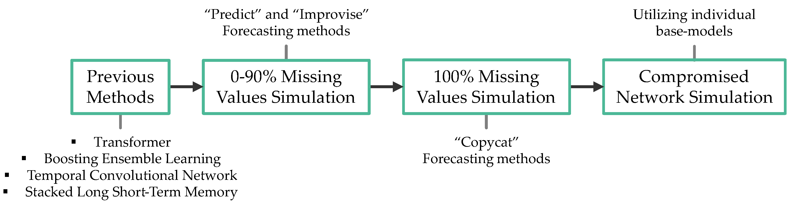
4.1. Overview

This section presents the Transformer, boosting ensemble learning, TCN, and stacked LSTM as the previous methods to compare against CIP in forecasting the electricity load in zone $WEST$, forecasting outcome on different percentages of simulated MV, and the forecasting outcome when part of the CIP networks was offline due to the DDoS attack. Figure 13 shows the high-level summary for the previous methods, various MV percentages simulation and compromised network simulation.

4.2. Previous Methods

4.2.1. Transformer

Figure 14 shows the Transformer model implementation to forecast the electricity load in zone $WEST$, where the head_size represents the size of the attention heads, the num_head represents the number of attention heads in the multi-head attention layer, the ff_dim represents the size of the feed-forward layer inside the Transformer block, and the num_transformer_blocks as the number of Transformer blocks stacked in the model. In addition, the mlp_units represents the number of units in each fully connected layer of the multi-layer perceptron (MLP) following the Transformer blocks, mlp_dropout represents the dropout rate in the output of each fully connected layer in the MLP, and ovl_dropout represents the dropout rate in the output of the multi-head attention layer in each Transformer block.

As the Transformer model tends to overfit when trained with ten training datasets that have the same electricity load data with varying MV percentages prepared in Section 2.2, we took the training dataset with 0% of MV and simulated 25% of MV in it instead, which is the technique we used in our previous study to prevent overfitting. Models that exhibit overfitting will show unexpected behavior, where the forecasting accuracy will only increase as the MV percentages increase, making it unpractical for normal operations.

We trained the Transformer model with a batch size of 1000, 100 training epoch, 0.0001 learning rate for Adam, and the early stop set to 3 with 0.0001 as the minimum observable improvement on MSE.

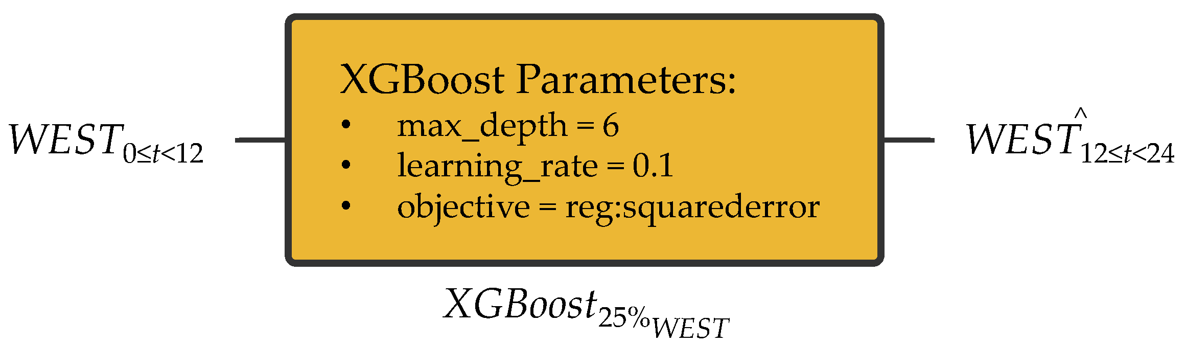
4.2.2. Boosting Ensemble Learning

Figure 15 shows the boosting ensemble learning model implementation to forecast the electricity load in zone $WEST$. We implemented the boosting ensemble learning based on eXtreme Gradient Boosting (XGBoost) [41], where the max_depth represents the maximum depth of each tree in the boosting process, the learning_rate represents the step size at each iteration while moving toward a minimum of the loss function, and the objective as reg:squarederror represents the specified learning task and objective function, which show the model trained for regression problem to minimize the MSE.

Similar to the Transformer model, even with the early stop function set to stop the training when the MSE score no longer improves after three times, the XGBoost model exhibits overfitting tendencies when trained with ten training datasets with varying MV percentages prepared in Section 2.2. We solved this issue using the training dataset with 25% of MV used on the Transformer model to train the XGBoost model in 500 epochs.

4.2.3. Temporal Convolutional Network

Figure 16 shows the TCN-based model implementation to forecast the electricity load in zone $WEST$, where the first and second convolutional layers use 64 filters, kernel size set to 3, and padding set to causal to ensure the current output depends only on the current and past input, while the third dense layer has 50 units. The convolutional and the dense layers use rectified linear units (ReLU) as the activation function.

As the TCN model does not exhibit the overfitting behavior shown in the Transformer and XGBoost model, we used ten training datasets that have the same electricity load data with varying MV percentages prepared in Section 2.2, concatenated into one long sequence to train the TCN model with a batch size of 1000, 100 training epoch, 0.0001 learning rate for Adam, and the early stop set to 3 with 0.0001 as the minimum observable improvement on MSE.

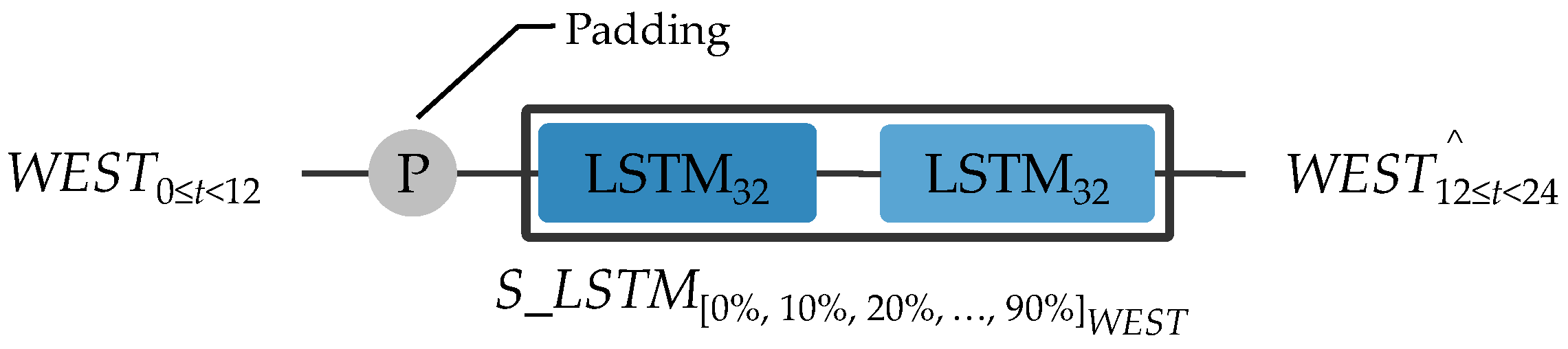
4.2.4. Stacked Long Short-Term Memory

Figure 17 shows the stacked LSTM-based model implementation to forecast the electricity load in zone $WEST$, where the first and second LSTM layers use 32 units and TanH as the activation function.

Similar to the TCN model, we use ten training datasets that have the same electricity load data with varying MV percentages prepared in Section 2.2, concatenated into one long sequence to train the LSTM model with a batch size of 1000, 100 training epoch, 0.0001 learning rate for Adam, and the early stop set to 3 with 0.0001 as the minimum observable improvement on MSE.

4.3. 0–90% Missing Values Simulation

In this test, we used evaluation datasets with different MV percentages prepared in Section 2.2 to evaluate the forecasting accuracy of CIP, TCN, boosting ensemble learning, Transformer, and stacked LSTM models on the electricity load in zone $WEST$.

Table 4. Coefficient of determination ($r^2$) scores comparison between multiple forecasting methods on different missing values percentages in zone $WEST$.

MV [%]	CIP	TCN	Boosting	Transformer	Stacked LSTM
0	0.98831	0.98567	0.98523	0.93445	0.98626
10	0.98501	0.98465	0.98478	0.91115	0.98579
20	0.98498	0.98381	0.98392	0.89104	0.98518
30	0.98492	0.98273	0.98241	0.87363	0.98421
40	0.98478	0.98159	0.97655	0.85770	0.98311
50	0.98410	0.97856	0.95719	0.36864	0.98029
60	0.98214	0.97292	0.91396	−1.53278	0.97468
70	0.97727	0.95687	0.75946	−11.5464	0.95892
80	0.96225	0.88543	0.33560	−74.1568	0.88781
90	0.89345	0.65085	−0.66817	−296.831	0.65736
Average	0.97272	0.93631	0.72109	−37.92314	0.93836

and Figure 18 show the $r^2$ forecasting scores on zone $WEST$. We used $r^2$ to calculate the forecasting accuracy, as the ease of interpretability gives us a generalized idea of how similar the forecast would match with the plotted real values [42].

With 0% of MV in zones $WEST$, $GENESE$, and $CENTRL$, CIP utilizes the “predict” forecasting method in the Level 0 network to forecast the electricity load, which achieves the highest $r^2$ score of 0.98831 when compared to the previous forecasting methods. As the MV percentages in $WEST$, $GENESE$, and $CENTRL$ rise from 1% to 90%, CIP utilizes the “improvise” forecasting method to combine the forecast from base models in Level 0 network and fine-tune them into one forecast using the meta-model in Level 1 network, which yields $r^2$ score of 0.96225 with 80% of MV in the independent variables. In contrast, none of the previous forecasting methods achieve $r^2$ score of 0.9 and above with 80% of MV. Even with 90% of MV, the $r^2$ score on CIP only falls to 0.89345, showing the resilience of our proposed method against MV, as the $r^2$ scores for the previous methods already fall below 0.7.

Examining the forecasting accuracies for the previous forecasting methods, TCN and stacked LSTM models are the only previous methods that equally perform well and could maintain a $r^2$ score of 0.95 with 70% of MV in the independent variable. These results show the TCN and stacked LSTM capability in capturing the dependencies in the independent variables with either convolutional layers or gating mechanisms without MV negatively affecting the forecast.

Table 5. Root-mean-square error scores comparison between multiple forecasting methods on different missing values percentages.

MV [%]	CIP	TCN	Boosting	Transformer	Stacked LSTM
0	0.03137	0.03433	0.03480	0.07452	0.03355
10	0.03555	0.03557	0.03535	0.08756	0.03413
20	0.03565	0.03656	0.03637	0.09733	0.03488
30	0.03573	0.03779	0.03814	0.10501	0.03605
40	0.03588	0.03903	0.04443	0.11154	0.03733
50	0.03670	0.04223	0.06089	0.23587	0.04044
60	0.03899	0.04779	0.08686	0.47234	0.04616
70	0.04409	0.06083	0.14554	1.05115	0.05935
80	0.05712	0.10024	0.24196	2.57265	0.09918
90	0.09663	0.17537	0.38340	5.12129	0.17371
Average	0.04477	0.06097	0.11077	0.99293	0.05948

and Figure 19 show the RMSE forecasting scores on zone $WEST$, which support the results shown in Table 4 and Figure 18 where CIP surpass previous forecasting methods in resiliency against MV.

4.4. 100% Missing Values Simulation

In this test, we set the MV percentages to 100% for zones $WEST$, $GENESE$, and $CENTRL$. As it is impossible to forecast with 100% of MV, CIP relies on the “copycat” forecasting method to reconstruct the forecast for zone $WEST$, where the MV percentages in each zone rise from 0% to 90% with a 10% increment.

Table 6. Coefficient of determination ($r^2$) and root-mean-square error scores obtained from the reconstructed electricity load forecast for zone $WEST$.

MV [%]	${\mathit{r}}^2$	RMSE
0	0.81445	0.12785
10	0.76918	0.14261
20	0.76517	0.14385
30	0.76375	0.14428
40	0.75983	0.14548
50	0.75710	0.14630
60	0.75839	0.14591
70	0.76295	0.14453
80	0.76616	0.14354
90	0.74013	0.15129

and Figure 20 show the results where CIP obtained an $r^2$ score of 0.81445 with 0% of MV. In addition, the score only drops to 0.74013 with 90% of MV, which is a 9.56142% degradation.

Although the forecast accuracy using the “copycat” method is inferior, it constructed the forecast in zone $WEST$ even with 100% of MV in $WEST$, $GENESE$, and $CENTRL$, which is unattainable with previous methods.

4.5. Compromised Network Simulation

In the final test, we simulated a scenario where Level 1 and Level 2 networks in $CI{P}_{WEST}$ are offline. Using the base model trained with an MV percentage close to the MV percentage in the input data, we could obtain an accurate prediction similar to the meta-model in Level 1.

Table 7. Coefficient of determination ($r^2$) and root-mean-square error scores obtained from the individual base-model load forecast for zone $WEST$.

MV [%]	${\mathit{r}}^2$	RMSE
0	0.98826	0.03141
10	0.98739	0.03245
20	0.98704	0.03294
30	0.98440	0.03614
40	0.98409	0.03644
50	0.98235	0.03846
60	0.97132	0.04917
70	0.97086	0.04997
80	0.95744	0.06045
90	0.88504	0.10029

and Figure 21 show the forecasting outcome using the individual base models.

5. Conclusions

The digitalization of essential infrastructures in smart cities introduces new challenges. With the increasing threat of cyberattacks targeting the electricity infrastructure, we must design countermeasures to ensure the service will not be interrupted, which could negatively impact the economy and other essential services. We proposed CIP, a distributed forecasting network that could handle a high percentage of MV and solve the SPoF vulnerability to prevent interruption. CIP works by utilizing multi-level networks to forecast the electricity load based on the MV percentage in the input sequence. When there is no MV, we rely solely on the base model in Level 0 to “predict” the electricity load to reduce unnecessary computation, with an $r^2$ score of 0.98831. As the MV rises from 1% to 90%, CIP utilizes the meta-model in the Level 1 network to “improvise” the “prediction” from the base models from Level 0, which allows our proposed method to handle up to 80% of MV while maintaining $r^2$ score of 0.96225. Even when one of the data sources providing the electricity load data is offline, we reconstruct the forecast using a meta-model in Level 2 to create a “copycat” forecast, which CIP reconstructs from electricity load data from other zones with $r^2$ score of 0.81445. Finally, as our proposed forecast method is modular, the predictions from the individual base models trained with the MV percentage close to the input data are accessible with comparable accuracy with the meta-model in Level 1.

For future works, we aim to expand the capability of our CIP to handle concept drift by integrating our previous research using radian scaling [43], detecting data falsification, and improving the forecasting accuracy in Level 2 using different types of data, as our current research is limited only to the electricity load data from other zones.

References

- Nti, I.K.; Teimeh, M.; Nyarko-Boateng, O.; Adekoya, A.F. Electricity load forecasting: A systematic review. J. Electr. Syst. Inf. Technol. 2020, 7, 13. [Google Scholar] [CrossRef]
- Kruse, J.; Schäfer, B.; Witthaut, D. Predictability of Power Grid Frequency. IEEE Access 2020, 8, 149435–149446. [Google Scholar] [CrossRef]
- Sweeney, C.; Bessa, R.J.; Browell, J.; Pinson, P. The future of forecasting for renewable energy. WIREs Energy Environ. 2020, 9, e365. [Google Scholar] [CrossRef]
- Klyuev, R.V.; Morgoev, I.D.; Morgoeva, A.D.; Gavrina, O.A.; Martyushev, N.V.; Efremenkov, E.A.; Mengxu, Q. Methods of Forecasting Electric Energy Consumption: A Literature Review. Energies 2022, 15, 8919. [Google Scholar] [CrossRef]
- Sue Wing, I.; Rose, A.Z. Economic consequence analysis of electric power infrastructure disruptions: General equilibrium approaches. Energy Econ. 2020, 89, 104756. [Google Scholar] [CrossRef]
- IBM Security. X-Force Threat Intelligence Index 2023. Available online: https://www.ibm.com/reports/threat-intelligence/ (accessed on 21 November 2023).
- Li, Y.; Liu, Q. A comprehensive review study of cyber-attacks and cyber security; Emerging trends and recent developments. Energy Rep. 2021, 7, 8176–8186. [Google Scholar] [CrossRef]
- Azure Network Security Team. 2022 in Review: DDoS Attack Trends and Insights. Microsoft. Available online: https://www.microsoft.com/en-us/security/blog/2023/02/21/2022-in-review-ddos-attack-trends-and-insights/ (accessed on 10 August 2023).
- Gjesvik, L.; Szulecki, K. Interpreting cyber-energy-security events: Experts, social imaginaries, and policy discourses around the 2016 Ukraine blackout. Eur. Secur. 2023, 32, 104–124. [Google Scholar] [CrossRef]
- Rodrigues, F.; Cardeira, C.; Calado, J.M.F.; Melicio, R. Short-Term Load Forecasting of Electricity Demand for the Residential Sector Based on Modelling Techniques: A Systematic Review. Energies 2023, 16, 4098. [Google Scholar] [CrossRef]
- Wazirali, R.; Yaghoubi, E.; Abujazar, M.S.S.; Ahmad, R.; Vakili, A.H. State-of-the-art review on energy and load forecasting in microgrids using artificial neural networks, machine learning, and deep learning techniques. Electr. Power Syst. Res. 2023, 225, 109792. [Google Scholar] [CrossRef]
- Jung, S.; Moon, J.; Park, S.; Rho, S.; Baik, S.W.; Hwang, E. Bagging Ensemble of Multilayer Perceptrons for Missing Electricity Consumption Data Imputation. Sensors 2020, 20, 1772. [Google Scholar] [CrossRef] [PubMed]
- Rodenburg, F.J.; Sawada, Y.; Hayashi, N. Improving RNN Performance by Modelling Informative Missingness with Combined Indicators. Appl. Sci. 2019, 9, 1623. [Google Scholar] [CrossRef]
- Myllyaho, L.; Raatikainen, M.; Männistö, T.; Nurminen, J.K.; Mikkonen, T. On misbehaviour and fault tolerance in machine learning systems. J. Syst. Softw. 2022, 183, 111096. [Google Scholar] [CrossRef]
- Dehghani, M.; Yazdanparast, Z. From distributed machine to distributed deep learning: A comprehensive survey. J. Big Data 2023, 10, 158. [Google Scholar] [CrossRef]
- Drainakis, G.; Pantazopoulos, P.; Katsaros, K.V.; Sourlas, V.; Amditis, A.; Kaklamani, D.I. From centralized to Federated Learning: Exploring performance and end-to-end resource consumption. Comput. Netw. 2023, 225, 109657. [Google Scholar] [CrossRef]
- Aguilar Madrid, E.; Antonio, N. Short-Term Electricity Load Forecasting with Machine Learning. Information 2021, 12, 50. [Google Scholar] [CrossRef]
- Jiang, W. Deep learning based short-term load forecasting incorporating calendar and weather information. Internet Technol. Lett. 2022, 5, e383. [Google Scholar] [CrossRef]
- New York Independent System Operator. Load Data. Available online: https://www.nyiso.com/load-data/ (accessed on 18 July 2023).
- Puth, M.-T.; Neuhäuser, M.; Ruxton, G.D. Effective use of Spearman’s and Kendall’s correlation coefficients for association between two measured traits. Anim. Behav. 2015, 102, 77–84. [Google Scholar] [CrossRef]
- Makowski, D.; Ben-Shachar, M.S.; Patil, I.; Lüdecke, D. Methods and algorithms for correlation analysis in R. J. Open Source Softw. 2020, 5, 2306. [Google Scholar] [CrossRef]
- Pandas 2.1.3. 2023. Available online: https://pandas.pydata.org (accessed on 18 November 2023).
- Shojaie, A.; Fox, E.B. Granger Causality: A Review and Recent Advances. Annu. Rev. Stat. Its Appl. 2022, 9, 289–319. [Google Scholar] [CrossRef] [PubMed]
- Statsmodels 0.14.0. 2023. Available online: https://www.statsmodels.org (accessed on 17 June 2023).
- Kadhim, Z.S.; Abdullah, H.S.; Ghathwan, K.I. Artificial Neural Network Hyperparameters Optimization: A Survey. Int. J. Online Biomed. Eng. 2022, 18, 59–87. [Google Scholar] [CrossRef]
- Wu, J.; Chen, X.-Y.; Zhang, H.; Xiong, L.-D.; Lei, H.; Deng, S.-H. Hyperparameter Optimization for Machine Learning Models Based on Bayesian Optimization. J. Electron. Sci. Technol. 2019, 17, 26–40. [Google Scholar]
- Keras Tuner 1.4.6. 2023. Available online: https://github.com/keras-team/keras-tuner (accessed on 3 December 2023).
- TensorFlow 2.13.1. 2023. Available online: https://www.tensorflow.org (accessed on 4 September 2023).
- Shafieian, S.; Zulkernine, M. Multi-layer stacking ensemble learners for low footprint network intrusion detection. Complex Intell. Syst. 2023, 9, 3787–3799. [Google Scholar] [CrossRef]
- Abumohsen, M.; Owda, A.Y.; Owda, M. Electrical Load Forecasting Using LSTM, GRU, and RNN Algorithms. Energies 2023, 16, 2283. [Google Scholar] [CrossRef]
- Wan, R.; Mei, S.; Wang, J.; Liu, M.; Yang, F. Multivariate Temporal Convolutional Network: A Deep Neural Networks Approach for Multivariate Time Series Forecasting. Electronics 2019, 8, 876. [Google Scholar] [CrossRef]
- Lara-Benítez, P.; Carranza-García, M.; Luna-Romera, J.M.; Riquelme, J.C. Temporal Convolutional Networks Applied to Energy-Related Time Series Forecasting. Appl. Sci. 2020, 10, 2322. [Google Scholar] [CrossRef]
- Zhao, Z.; Xia, C.; Chi, L.; Chang, X.; Li, W.; Yang, T.; Zomaya, A.Y. Short-Term Load Forecasting Based on the Transformer Model. Information 2021, 12, 516. [Google Scholar] [CrossRef]
- L’Heureux, A.; Grolinger, K.; Capretz, M.A.M. Transformer-Based Model for Electrical Load Forecasting. Energies 2022, 15, 4993. [Google Scholar] [CrossRef]
- Stratigakos, A.; Andrianesis, P.; Michiorri, A.; Kariniotakis, G. Towards Resilient Energy Forecasting: A Robust Optimization Approach. IEEE Trans. Smart Grid 2024, 15, 874–885. [Google Scholar] [CrossRef]
- Mienye, I.D.; Sun, Y. A Survey of Ensemble Learning: Concepts, Algorithms, Applications, and Prospects. IEEE Access 2022, 10, 99129–99149. [Google Scholar] [CrossRef]
- Grotmol, G.; Furdal, E.H.; Dalal, N.; Ottesen, A.L.; Rørvik, E.-L.H.; Mølnå, M.; Sizov, G.; Gundersen, O.E. A robust and scalable stacked ensemble for day-ahead forecasting of distribution network losses. In Proceedings of the AAAI Conference on Artificial Intelligence, Washington, DC, USA, 7–14 February 2023; Volume 37, pp. 15503–15511. [Google Scholar]
- Gupta, H.; Agarwal, P.; Gupta, K.; Baliarsingh, S.; Vyas, O.P.; Puliafito, A. FedGrid: A Secure Framework with Federated Learning for Energy Optimization in the Smart Grid. Energies 2023, 16, 8097. [Google Scholar] [CrossRef]
- Shi, B.; Zhou, X.; Li, P.; Ma, W.; Pan, N. An IHPO-WNN-Based Federated Learning System for Area-Wide Power Load Forecasting Considering Data Security Protection. Energies 2023, 16, 6921. [Google Scholar] [CrossRef]
- Shi, Y.; Xu, X. Deep Federated Adaptation: An Adaptative Residential Load Forecasting Approach with Federated Learning. Sensors 2022, 22, 3. [Google Scholar] [CrossRef] [PubMed]
- eXtreme Gradient Boosting 2.0.2. 2023. Available online: https://github.com/dmlc/xgboost (accessed on 19 November 2023).
- Chicco, D.; Warrens, M.J.; Jurman, G. The coefficient of determination R-squared is more informative than SMAPE, MAE, MAPE, MSE and RMSE in regression analysis evaluation. PeerJ Comput. Sci. 2021, 7, e623. [Google Scholar] [CrossRef] [PubMed]
- Bin Kamilin, M.H.; Yamaguchi, S.; Bin Ahmadon, M.A. Radian Scaling: A Novel Approach to Preventing Concept Drift in Electricity Load Prediction. In Proceedings of the 2023 IEEE International Conference on Consumer Electronics-Asia (ICCE-Asia), Busan, Republic of Korea, 23–25 October 2023; pp. 1–4. [Google Scholar]