Abstract
Advancements in AI have elevated speech recognition, with convolutional neural networks (CNNs) proving effective in processing spectrogram-transformed speech signals. CNNs, with lower parameters and higher accuracy compared to traditional models, are particularly efficient for deployment on storage-limited embedded devices. Artificial neural networks excel in predicting inputs within their expected output range but struggle with anomalies. This is usually harmful to a speech recognition system. In this paper, the neural network classifier for speech recognition is trained with a “negative branch” method, incorporating directional regularization with out-of-distribution training data, allowing it to maintain a high confidence score to the input within distribution while expressing a low confidence score to the anomaly input. It can enhance the performance of anomaly detection of the classifier, addressing issues like misclassifying the speech command that is out of the distribution. The result of the experiment suggests that the accuracy of the CNN model will not be affected by the regularization of the “negative branch”, and the performance of abnormal detection will be improved as the number of kernels of the convolutional layer increases.
1. Introduction
In recent years, the rapid development of artificial intelligence and deep learning technologies has led to the widespread application of speech recognition as a vital human–computer interaction technology in various fields [1,2,3,4]. Prominent AI-powered speech recognition systems include Speech-to-Text from Google, Azure Speech Services from Microsoft, Siri from Apple, Alexa from Amazon, etc. These systems excel in tasks such as real-time transcription and voice commands.
Convolutional neural networks (CNNs) have not only achieved significant success in image recognition but have also demonstrated outstanding performance in speech recognition [5]. Feature extraction algorithms for speech signals can transform them into two-dimensional spectrograms, and CNNs can classify speech signals in a manner analogous to image classification [5]. Compared to popular architectures, like Deep Neural Networks (DNNs) [2] and Recurrent Neural Networks (RNNs) [6,7], convolutional neural networks (CNNs) exhibit a smaller parameter count when handling inputs with numerous features [8]. This is attributed to strategies like parameter sharing, local receptive fields, and sparse connectivity, reducing model complexity. These characteristics make CNNs more efficient on embedded devices with limited memory. In contrast, traditional DNNs often require more parameters due to fully connected layers. DNNs focus on global features without weight sharing mechanisms; they are sensitive to spatial locations, causing a higher parameter count, and they are less suitable to be deployed on memory-limited embedded systems.
The utilization of embedded devices for speech recognition offers diverse advantages [9]. Embedded devices typically feature lower power consumption and excellent real-time performance, allowing for swift responses to voice commands and an enhanced user experience. The compact design of embedded devices enables seamless integration into various applications, such as smart homes and health monitoring, providing a more convenient interaction through speech recognition. Real-time processing stands out as an additional advantage; by conducting speech recognition processing on embedded devices, the need for transmitting data to the cloud is eliminated, reducing reliance on network connections and safeguarding user privacy.
However, deploying neural networks on embedded devices presents several challenges. Embedded devices often have limited memory footprint and computational power. Artificial neural networks typically come with a substantial number of parameters, resulting in significant memory requirements. Meanwhile, the inference of neuron networks is usually computationally expensive. Therefore, the neural networks that are suitable to be deployed on embedded devices must strike a balance; they should not be overly complex and with a relatively small parameter count, yet this constraint should not compromise their inherent performance.
There is another challenge for AI-based speech recognition systems. Artificial neural networks exhibit robust performance in predicting the inputs within their output distribution [10]. However, the range of input is much wider than the output distribution of a neural network in practical applications. When faced with an input outside this distribution, they often run the risk of producing a high confidence score and misclassifying it as belonging to one of the categories within their expected output [11,12]. In other words, artificial neural networks usually show suboptimal performance in anomaly detection. Considering the practical application and the safety of an AI-based system, a neural network classifier should be capable to detect and reject the anomaly input [12]. For example, consider a speech recognition system based on artificial neural networks that identify specific keywords. If a user speaks the words outside of its predefined set, the system needs to accurately recognize that those words do not match the known keywords. But, artificial neural networks often struggle with making this distinction and will mistakenly classify it as one of the defined keywords. This can lead to unintended actions being triggered, which is typically detrimental to a speech recognition system.
To address these challenges, several approaches to detect out-of-distribution input have been proposed. Ref. [13] presented a simple baseline using the probabilities from the softmax distribution. Ref. [14] proposed a method that trains a neural network using learning confidence estimates, without using any out-of-distribution examples. In recent neural network research, studies on stability, Hopf bifurcation, and dynamics encompassed fractional-order three-triangle multi-delayed networks [15], fractional delayed bidirectional associative memory (BAM) networks [16], and fractional-order Cohen–Grossberg networks with three delays [17]. Additionally, a breakthrough in understanding bifurcations in fractional-order bidirectional associative memory networks was achieved, focusing on self-regulating parameters [18].
In this paper, an approach called “negative branch” is employed for the training of artificial neural networks. In each iteration of traditional gradient descent, a directional regularization is added using training data that are outside the output distribution. The main contributions of this paper are as follows:
- A single-word speech recognition based on an embedded system using CNNs is introduced. The system is not always turned on and it is triggered only when speech activity is detected.
- The “negative branch” method is introduced, using out-of-distribution examples to perform regularization during training. Testing of this training approach demonstrated its capability to improve the anomaly detection performance of artificial neural networks compared to traditional methods. Additionally, further experiments were conducted to explore the factors influencing the performance of models trained using this method.
2. System
2.1. Speech Recognition System
As shown in Figure 1, the speech recognition system consists of three main sections: the endpoint detection program (EPD), the digital signal processing program (DSP), and the convolutional neural network. In this system, speech recognition remains deactivated until it is triggered. An endpoint detection program is used to detect speech activity. Speech recognition is only triggered when speech activity is detected by the endpoint detection program. When speech recognition is triggered, the DSP program is responsible for performing MFCC computation for the audio signal that is captured by the microphone, transforming the raw audio signal in the time domain into a n × n spectrogram image that contains the extracted features on both the time and frequency domain. The computed spectrogram images will be fed into the convolutional neuron network that is deployed on the embedded device. The network will perform classification for the given input and finally, the result of the voice recognition will be yield. Then, the speech recognition will be off until another speech activity is detected.
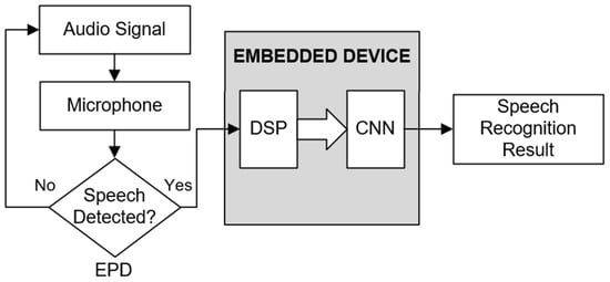
Figure 1.
Overall block diagram of the speech recognition system.
2.2. Endpoint Detection
The speech recognition is off when the device is in a silent environment, and it will be triggered by the endpoint detection program. As shown in Figure 2, when the speech recognition is not being triggered, only the ADC is on, and it keeps sampling the output voltage of the analog microphone. The ZCR and RMSE of the sampled frame, which included 1024 sample data, will be calculated. A threshold value for the ZCR and RMSE will be set. If both the ZCR and RMSE of the frame exceed the given thresholds, it will be considered that a speech signal is detected, and speech recognition will be triggered.
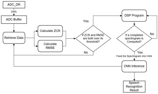
Figure 2.
Endpoint detection program.
There are two benchmarks in the endpoint detection program in this project: the Zero Crossing Rate (ZCR) and root mean square energy (RMSE) of the sound signal in a short period.
Zero Crossing Rate (ZCR):
The ZCR is the rate at which the sound signal crosses the “zero-crossing” line; in other words, changes from positive to negative, or vice versa. The speech signals typically have a higher ZCR. Therefore, speech activity can be detected by setting a ZCR threshold. The Zero Crossing Rate (ZCR) for an audio signal is calculated using the formula:
In this formula, t is the time variable denoting the index of the sample data, K is the size of the frame, and s(k) represents the sample value at time k. The summation calculates the differences in signs between adjacent samples within a frame, representing the number of zero crossings. The 1/2 term normalizes the zero crossing rate by considering that each change in sign corresponds to two zero crossings.
Root Mean Square Energy (RMSE):
The RMSE is a benchmark that measures the overall energy of a signal over a short period. Speech signals typically have higher energy during speech and lower energy during pauses or silence. Therefore, the change in the RMSE can reflect the difference in energy between speech and non-speech segments. At the beginning of a speech signal, the RMSE will increase significantly. The starting point of a speech signal can be determined by detecting the rise in the RMSE.
The summation calculates the sum of squared sample values s(k) within a frame. It is normalized by incorporating the size of the frame K. It is square rooted to obtain the RMSE value during a short period. It is commonly employed in signal processing for feature extraction and intensity analysis.
2.3. Digitial Signal Processing for Feature Extraction
The purpose of the digital signal processing program is to transform the continuous, time domain speech signal that is recorded by the microphone into an n × n MFCC spectrogram image [19]. The final output of the program contains features from both the time and frequency domains of the speech signal. This spectrogram serves as the input for the convolutional neural network (CNN), which is responsible for feature extraction and classification. The CNN effectively achieves the functionality of speech recognition. As shown in Figure 3, from left to right, a comprehensive digital signal processing program is divided into several parts, including sampling, frame segmentation, normalization, fast Fourier transform (FFT), Mel filter bank filtering, and MFCC computation.
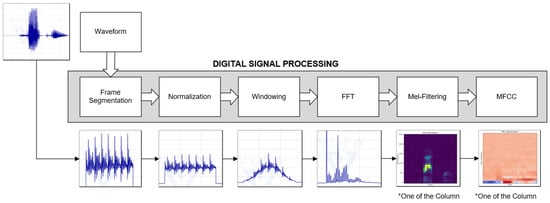
Figure 3.
Digital signal processing program for feature extraction.
Most of the sound signals in real life are non-stationary in the time domain, and the frequency and amplitude both change with time. A series of sound signal samples could be approximately treated as stationary signals if the sound signal is divided into short frames. The raw audio signal is sampled by the ADC with a sample rate of 16 k. Each of the frames contains 1024 sampled data, corresponding to 64 ms in the time domain, and there is a 50% overlapping between every two conjugate frames. In other words, the hop length of the frame is 512. After obtaining the sampled data of a frame, the 1024 data in the frame will be normalized and multiplied with a Hamming window function. Continuing with the procedure, the program processes the 1024 data points within each frame using FFT calculations, converting the time series data into a frequency–domain spectrum. Subsequently, the spectrum undergoes filtration through a set of Mel filter banks to obtain the extracted frequency domain feature coefficients. The coefficients are transformed into a logarithmic scale and subjected to a discrete cosine transform, resulting in the derivation of 20 MFCC coefficients. These coefficients will become one of the columns of an MFCC spectrogram. A complete MFCC spectrogram includes 30 columns, representing the extracted feature of 30 consecutive data frames, with a corresponding period of approximately 992 milliseconds. The MFCC spectrogram can be considered as a 2D image and will be fed into the convolutional neuron network.
2.4. Convolution Neuron Network
Convolutional neural networks (CNNs) are utilized to perform additional feature extraction and classification on Mel-Frequency Cepstral Coefficient (MFCC) spectrograms computed by DSP programs. The initial layers of a CNN typically comprise convolutional layers responsible for feature extraction, followed by fully connected layers that are connected to process the extracted features for classification.
As shown in Table 1, the baseline CNN model contains three convolutional pooling layers. All the convolutional layers use 5 × 5 kernels, and all the sizes of kernels for the pooling layer are 2 × 2. The number of kernels for the first, second, and third layer are 10, 20, and 30, respectively. The output of the last convolutional pooling layer is flattened into a one-dimensional vector and connected by the fully connected (FC) layer for classification. The last fully connected layer uses a softmax layer with temperature scaling [20] as its activation function, and the rest of the convolutional layers and fully connected layers use the rectified linear unit (Relu) as their activation function. Batch normalization is added to accelerate the training of the model [21]. The total parameter count for the baseline model is 64,628. The baseline model is denoted as cnn_55_10_20_40.

Table 1.
Structure of the baseline CNN model.
2.5. Hardware Description
The STM32H743VIT6 microcontroller from ST Microelectronic is chosen to handle the digital signal processing task and the computation of the convolutional neuron network. The key specification of the STM32H743VIT6 microcontroller is shown in Table 2. This model is positioned as one of the high-end microcontrollers of STMicroelectronics using a Cortex-M7 processer, distinguished by its relatively high main frequency and powerful computational capabilities. The neuron network is implemented by the X-Cube AI expansion pack for STM32CubeMX.
Table 2.
Specification of the microcontroller.
3. Method
3.1. Dataset
The Speech Commands dataset [22] from Tensorflow was chosen for training and evaluating the model. It contains 30 different recorded single-word commands in wave format. Among them, 8 classes were treated as the output categories of the CNN model, which are considered as “positive” data. They are “go”, “stop”, ”forward”, “backward”, “up”, “down”, “left”, and “right”. The rest of the 22 classes were considered as “negative” data.
As shown in Figure 4, the wave files were stored in a micro-SD card. The FatFs file system has been transplanted to the STM32 platform to facilitate the retrieval of wave files from the micro-SD card. The wave files in this dataset are monaural, featuring a data depth of 16 bits and a sampling rate of 16,000, which is identical to the setting of the ADC in the DSP program. As a result, the FatFs file system serves the purpose of “sampling” the audio data from the wave files. Subsequently, the DSP program will compute a 20 × 30 MFCC spectrogram corresponding to each wave file. Finally, the processed data are transmitted to a PC via serial communication and saved locally in the form of .npy files. Using the predeveloped DSP program in STM32 to create a dataset can ensure that the trained CNN model is compatible with the MFCC spectrogram computed by the DSP program. Each of the .npy files contains a 20 × 30 NumPy array, representing an MFCC spectrogram corresponding to a recorded voice command. There are a total of 7832 positive data and 11,395 negative data. Each of them was split into a training set and a test set with a ratio of 80:20. In the dataset, there is not any audio file in the “silent” class that is without any spoken word since speech recognition is triggered by a detected speech activity.
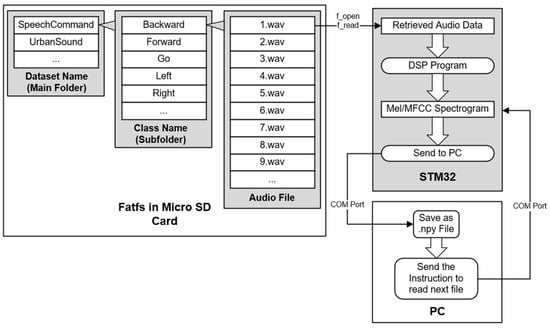
Figure 4.
Collecting dataset by “sampling” the wave files.
3.2. Training with Negative Branch
During the training of the model using the conventional mini-batch gradient descent method, in each iteration, the loss function is computed based on the training data within the model’s output distribution. Subsequently, the optimizer performs backpropagation and updates the parameters according to the calculated loss function. Once the model is trained properly, all the parameters are adapted to fit the training data provided that are within the model’s output distribution. The model will produce a high confidence score to input that is within the distribution. However, it will also produce a high confidence score for out-of-distribution input, which can be harmful in many situations.
The “negative branch” method involves an additional parameter update in each iteration of traditional mini-batch gradient descent. After the 1st update of the parameter, another loss function is computed using out-of-distribution training data. The optimizer then performs the 2nd backpropagation with the computed loss function and updates the parameter for the 2nd time. The “negative branch” idea is used to guide the neural network classifier to output high confidence for in-distribution inputs while assigning low confidence to out-of-distribution inputs. This approach aims to enhance the anomaly detection performance of the model without sacrificing its accuracy.
The dataset used for model training includes two distinct groups.
The first group consists of “positive” input data, corresponding to the eight classes of keywords that fall within the output categories of the neural network. This dataset is labeled with indices ranging from 0 to 7, corresponding to eight distinct categories within the output of the neural network classifier. The objective of this dataset is to ensure that the model accurately classifies inputs belonging to the specified output categories, minimizing the likelihood of misclassifying them as negative inputs.
The second group consists of “negative” input data, including the remaining 22 keywords from the Speech Command dataset that do not fall into the predefined 8 output categories of the neural network. All data in this group is labeled with 0. The objective of the negative training data is to minimize the probability output by the model when faces an out-of-distribution input and bring it closer to the expected value of “0”.
The model is trained using mini-batch stochastic gradient descent. The batch size of positive training data is denoted as , and the batch size of negative training data is denoted as . As shown in Figure 5, in each training iteration, positive input training data points and negative input data points are randomly sampled from the positive and negative training datasets, respectively.
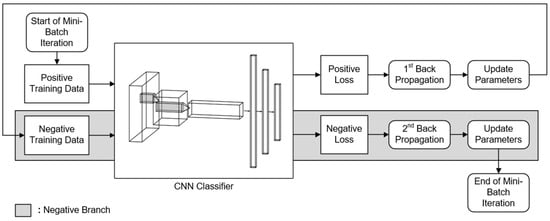
Figure 5.
Train the model with negative branch.
Initially, positive training data are fed into the model for forward propagation, thereby calculating the loss function . is defined as the cross-entropy loss between the model’s positive outputs and the given positive data. The formula is as follows:
where represents the predicted probability distribution and represents the true probability distribution. is the number of output categories.
After computing the positive loss function Lp, the optimizer will perform the 1st backpropagation and update the parameters of the model. Then, negative training data are fed into the model for forward propagation. The highest value of the model’s output distribution for each negative input data, denoted as , is extracted. In this context, the training process is conceptually simplified by treating the classifier as a binary classifier with only two classes: within the output distribution and outside the output distribution. can be treated as the probability that the binary classification model assigns negative input data falling within the output distribution of the multi-class classifier.
Consequently, the loss function for negative training data can be defined by binary cross-entropy. The labels for all the negative training data, denoted as are set to 0, corresponding to the “incorrect” label in the binary classification model. A hyperparameter λ is introduced to adjust the weights of the negative loss [14]. The weighted negative loss is denoted by .
Following the computation of the negative loss, the optimizer will perform the 2nd backpropagation and update the parameters of the model. The negative branch is equivalent to a directional regularization of a model at every iteration. Ideally, the model should assign a value of confidence score for an out-of-distribution input that is close to 0. The underlying mechanisms of the negative branch restrict the model from assigning a high confidence score to an out-of-distribution input by minimizing the negative loss function .
At this stage, a single mini-batch iteration is completed. The model has not only learned how to accurately classify positive input data but has also acquired the ability to reject negative input data.
3.3. Evaluation Matrix
DET Curve: The detection error tradeoff (DET) curves are used to illustrate the trade-off relationship between the False Reject Rate (FRR) and the False Alarm Rate (FAR). Specifically, the False Reject Rate (FRR) refers to the probability that the model mistakenly classifies negative input data as positive, while the False Alarm Rate (FAR) is the probability that the model mistakenly classifies positive input data as negative. In the context of DET curves, a lower AUC value is considered indicative of better model performance.
PR Curve: The (precision–recall) PR curve represents the relationship between precision rate and recall rate for a model. The precision rate is the proportion of samples predicted as positive by the model that belongs to the positive class, while the recall rate is the proportion of actual positive samples that are correctly predicted as positive by the model.
Output Distribution Histogram: The positive and negative test data are input into the model, and the highest probability output for each test datum is extracted. A histogram is plotted using these probabilities. The output distribution histogram of the model illustrates the probability distribution for a batch of positive and negative test data. It provides an intuitive comparison of the model’s performance by distinguishing between positive and negative data. In an ideal output distribution histogram, the majority of positive outputs would be situated in the high-probability positions on the right, while the majority of negative outputs would be located at the low-probability positions on the left.
Optimal Confidence Threshold: In the output of a single model inference, if the highest output probability is below the confidence threshold, the input for this inference is classified as a negative instance; otherwise, it is considered a positive instance. For a batch of test data, the true positive rate (TPR) represents the proportion of data classified as positive by the model among all positive test data, while the true negative rate (TNR) is the proportion of data classified as negative by the model among all negative test data. A higher value of the TPR and TNR indicates a better performance. The optimal confidence threshold can ensure the sum of the true negative rate (TNR) on the negative test set and the true positive rate (TPR) on the positive test set of a model are maximized. Moreover, the value of the confidence threshold can also indicate the balance of the model’s training. A “balanced” model typically exhibits an optimal confidence threshold of around 0.5. Throughout the training process, monitoring the optimal confidence threshold provides insights into the balance of the model. The optimal threshold on the test set can also be considered a reference for establishing the confidence threshold in the practical application.
4. Implementation Detail
During the training using the negative branch method, it was noticed that the optimal threshold of the output distribution of the model kept dropping as the training progressed. The model often ends up being excessively regularized at the later stage of the training, similar to the scenario in [14]. As shown in Figure 6, the model that is excessively regularized can only produce a low probability for the negative training data, and it is difficult to produce a high probability for the positive data. It will make the model lean toward the negative training data too much and eventually fail to accept the positive input data.
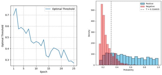
Figure 6.
The optimal threshold decreases rapidly during the training process (left), and the output distribution histogram of the baseline model is excessively regularized (right).
One way to address the problem is to reduce the level of regularization during the training [14]. This can be performed by adjusting the value of λ and the batch size of the negative data in mini-batch iterations. Figure 7 shows the changing of the optimal threshold during training with a lower value of λ and negative batch size. The regularization applied to the model has been reduced. In the output distribution histogram, most of the positive and negative output probability are located on the right and left sides, respectively.
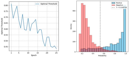
Figure 7.
The optimal threshold decreases slowly during the training process (left), and the output distribution histogram of the baseline model is properly regularized (right).
Ideally, the optimal threshold should hover around the value of 0.5. However, achieving this requires precise adjustment of hyperparameters during training. In the later stages of training, models with an optimal threshold of around 0.5 can be selected.
5. Experiment and Results
5.1. Comparison of the Traditional Method and Negative Branch Method
The baseline model was trained with the traditional method and the negative branch method, respectively. The initial learning rate is set to 0.0025. When the training of the model reaches a plateau, the learning rate will be scaled by a factor of 0.1.
Figure 8 shows that the test set accuracy of the model trained with the negative branch is slightly lower than the model trained with the traditional method during training. The result suggests that training with a negative branch introduces a very low impact on the accuracy of a model.
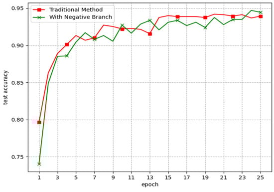
Figure 8.
The variation in accuracy on the positive test set of the model trained using traditional methods and the model trained using the negative branch during training.
Figure 9 and Figure 10 show the output distribution of the two models during training, respectively. In the case of using traditional training methods, the model not only exhibits high probability outputs for positive input data but also for negative input data. Furthermore, as the training progresses, the output probability for both positive and negative data tends to increase. Eventually, it makes the model fail to reject the out-of-distribution input and leads to poor performance of anomaly detection.
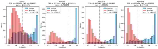
Figure 9.
During the training, the output distribution of the model trained using the negative branch is visualized in four histograms, corresponding to epochs 1, 6, 12, and 18.
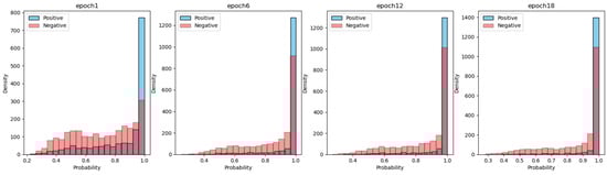
Figure 10.
During the training, the output distribution of the model trained using the traditional method is visualized in four histograms, corresponding to epochs 1, 6, 12, and 18.
The negative branch acts as a regularizer during training. It penalties the model and guides it to produce a low probability of negative input; at the same time, the number of high probability to positive input data produced by the model is reduced. The positive output distribution is less extreme than the model trained with the traditional method. The dashed line in the figure represents the optimal confidence threshold of the model. Under the threshold, the model will be able to accept most of the positive input data and simultaneously reject most of the negative data.
5.2. Number of Feature Maps
A higher number of parameters of CNNs typically leads to better performance [23]. One of the ways to increase the parameter count is to increase the number of feature maps per convolutional layer [4]. Three models with different numbers of feature maps per convolutional layer were trained with the negative branch method. They are denoted as cnn_55_5_8_15, cnn_55_10_20_40, and cnn_55_20_40_80, with the parameters counts of 19 k, 64 k, and 178 k, respectively (cnn_55_5_8_15 means that the kernel size of the convolution layer is 5 × 5, and 5, 8, and 15 represents the number of feature maps of the first, second, and third convolutional layer of the model, respectively).
It can be noticed in Figure 11 that as the number of feature maps increases, the model can reach a higher accuracy on the positive test set. The area under the DET curve decreases, which implies a better performance on anomaly detection. Meanwhile, the P-R curve of the model with a greater number of parameters dominates the P-R curve of the model with a smaller number of parameters. It was also noticed that the model with a parameter count of only 19 k is also able to reach a test accuracy of over 0.9, while the highest test accuracy of the model with 178 k parameters is slightly over 0.95.
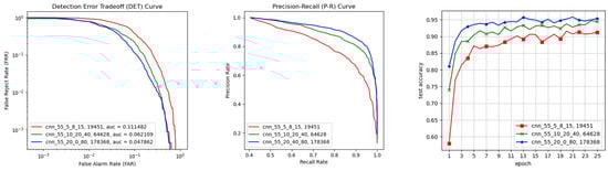
Figure 11.
Detection error tradeoff (DET) curves (left) for three models with different parameter counts, precision–recall (P-R) curves (center) for these three models, and the change in accuracy on the positive test set during training (right).
Figure 12 shows the output distributions of three models after training. It can be observed that as the number of feature maps increases, the output distributions of the models tend to be more concentrated toward both ends, and the sum of TPR and TNR under the optimal threshold increased. In other words, when provided with both positive and negative data during training, models with higher parameters can better distinguish between positive and negative data.
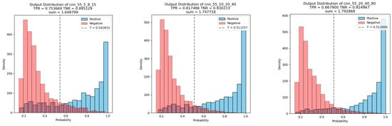
Figure 12.
Histograms of the output distribution for the three models with different parameter counts from left to right, corresponding to cnn_55_5_8_10, cnn_55_10_20_40, and cnn_55_20_40_80, respectively.
5.3. Deployment on a Microcontroller
The trained baseline model with 32-bit floating point number weights and activation was deployed on the STM32H743VIT6 microcontroller. Without any further compression, the weights of the model in C format take up 252.46 KiB in ROM, and the activation takes up 10.55 KiB of RAM.
The inference duration for the network model deployed on STM32H743VIT6 is 18.060 ms. Table 3 shows the computation time for each of the layers of the network that is running on STM32. This is performed by the “validate on Target” function of the X-Cube AI software pack of STM32 Cube-MX software (Version 10.6.1). This function can evaluate the performance of the deployed NN model. It uses a COM port to send instructions to the STM32 board and receive the result of validation. The result will be included in a report generated by the software, including the computation time of each of the layers of the deployed NN model. Notably, the computation time for the convolution pooling layer is the longest.
Table 3.
Computing duration of each layer in the deployed CNN model.
The diagram below shows the data in the output buffer of the neural (NN_Output) network on STM32H743VIT6 in debug mode, displayed in IDE software (Version 6.4). It also includes the label of the category (Predicted_Index) and the string, corresponding to the extracted maximum probability (str). For example, after a speech command “forward” is spoken, the DSP program is triggered by the endpoint detection program and will compute the MFCC spectrogram. Subsequently, the MFCC spectrogram was fed into the neural network for classification, and the probabilities for each category were stored in the output buffer. In the specific instance in Figure 13, the probability for category 2 is the highest at around 0.97, corresponding to the word “forward.” The output category and its associated probability for the inference were displayed on the LCD screen.
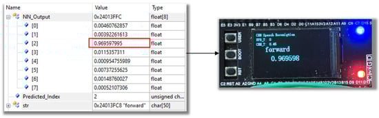
Figure 13.
The in-distribution result shown on the LCD display with its probability.
A confidence threshold value is set for the output of the networks to determine whether the output belongs to one of the designated output categories [13]. The final output is computed by a softmax layer, containing the probabilities for each output category for the current inference. If the value of maximum probability extracted from the output buffer is below the given threshold value, the corresponding output category will be marked as “other”, indicating that it does not fall into any specific output category. As shown in Figure 14, in this specific inference, the probabilities for each category in the output buffer are relatively evenly distributed. The threshold value was set at 0.45. The highest value from the output buffer is about 0.23, which was below the given threshold. Therefore, the output category for this inference was identified as “other.”
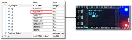
Figure 14.
The out-of-distribution result shown as “other” on the LCD display.
During actual testing, it was observed that the energy at the beginning of certain keyword command speech signals is relatively low, especially for the words that start with unvoiced sounds, like “forward” and “left”. The words that start with voiced sounds, such as “go” and “right”, exhibit lower zero crossing rates at the beginning of their speech signals. This often results in endpoint detection failing to precisely detect the speech activity at the moment the users utter these command words. The timestamp at which speech activity is detected commonly experiences a certain delay compared to the timestamp of the users who speak the command words. This leads to the loss of partial information on the speech command words in the MFCC spectrogram, ultimately affecting the accuracy of convolutional neural network classification. To address this issue, an offset needs to be introduced to compensate for the delay. As shown in Figure 15, when both the zero crossing rate and root mean square energy of a frame exceed the given threshold, as illustrated in the figure, the frame will be treated as the fourth frame in the MFCC spectrogram. The three offset frames before this frame serve as compensation for the detection delay, encompassing speech information that might be lost due to the delay. The remaining 26 frames will undergo feature extraction calculations. Finally, an MFCC spectrogram containing all the information from the speech signal is generated.
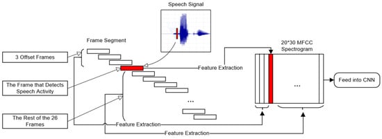
Figure 15.
Adding the offset frame to compensate for the delay in detection.
6. Conclusions and Discussion
In this paper, a convolutional neural network-based embedded speech recognition system is designed, with speech recognition only when triggered by an endpoint detection program; otherwise, it remains deactivated. To address the poor anomaly detection performance of the neural network classifier, a method called the “negative branch” is utilized for model training. The dataset is split into positive data that are within the output distribution and negative data that are out of the output distribution. During training, the model will fit the positive training data and learned to reject the negative training data at the same time. However, during training, the model is susceptible to over-regularization by the negative branch. To mitigate this issue, precise adjustment of certain hyperparameters related to model training is necessary. The results of the experiment suggested that for MFCC spectrograms, a convolutional neural network model with a very low parameter count can achieve high accuracy. Moreover, the anomaly detection capability improves as the model’s parameter count increases. In practical application, when the memory footprint of the device allows, it is encouraged to use a CNN structure with a higher number of convolutional kernels in each convolution layer, essentially opting for a broader network, to achieve a better performance of anomaly detection.
Under a similar parameter count, different model structures may have diverse impacts on the anomaly detection performance [4]. The impact of model quantization on anomaly detection performance also requires further investigation. Meanwhile, there is considerable room for improvement in the current training methods. For instance, the tendency toward over-regularization and the need to adjust hyperparameters during training make the training process more intricate and challenging. Additionally, ensuring that the model has iterated to an optimal state in the later stages of training is challenging. Additionally, in practical application scenarios, the model is likely to encounter inputs outside the distribution much more frequently than the negative data used during training. In the future, it may be worthwhile to consider introducing a more diverse set of data into the negative dataset for training.
Author Contributions
Conceptualization, resources, and software, J.C.; methodology, data curation, and supervision, T.H.T.; methodology, supervision, visualization, and formal analysis, C.L.K.; supervision, investigation, and funding acquisition, Y.Y.K. All authors have read and agreed to the published version of the manuscript.
Funding
This research received no external funding.
Data Availability Statement
The data presented in this study are available in this article.
Conflicts of Interest
The authors declare no conflicts of interest.
References
- Hinton, G.; Deng, L.; Yu, D.; Dahl, G.E.; Mohamed, A.; Jaitly, N.; Senior, A.; Vanhoucke, V.; Nguyen, P.; Sainath, T.N.; et al. Deep neural networks for acoustic modeling in speech recognition: The shared views of four research groups. IEEE Signal Process. Mag. 2012, 29, 82–97. [Google Scholar] [CrossRef]
- Sushan, P.; Anuradha, R. Speech Command Recognition using Artificial Neural Networks. JOIV Int. J. Inform. Vis. 2020, 4, 73–75. [Google Scholar]
- Chen, G.; Parada, C.; Heigold, G. Small-footprint keyword spotting using deep neural networks. In Proceedings of the 2014 IEEE International Conference on Acoustics, Speech and Signal Processing (ICASSP), Florence, Italy, 4–9 May 2014; pp. 4087–4091. [Google Scholar]
- Sainath, T.N.; Parada, C. Convolutional neural networks for small-footprint keyword spotting. Proc. Interspeech 2015, 1478–1482. [Google Scholar] [CrossRef]
- Li, X.; Zhou, Z. Speech Command Recognition with Convolutional Neural Network. CS229 Stanf. Educ. 2017, 31. [Google Scholar]
- Arik, S.O.; Kliegl, M.; Child, R.; Hestness, J.; Gibiansky, A.; Fougner, C.; Prenger, R.; Coates, A. Convolutional Recurrent Neural Networks for Small-Footprint Keyword Spotting. arXiv 2017, arXiv:1703.05390. [Google Scholar]
- Sun, M.; Raju, A.; Tucker, G.; Panchapagesan, S.; Fu, G.; Mandal, A.; Matsoukas, S.; Strom, N.; Vitaladevuni, S. Max-Pooling Loss Training of Long Short-Term Memory Networks for Small-Footprint Keyword Spotting. In Proceedings of the 2016 IEEE Spoken Language Technology Workshop (SLT), San Diego, CA, USA, 13–16 December 2016. [Google Scholar] [CrossRef]
- Abdel-Hamid, O.; Mohamed, A.; Jiang, H.; Penn, G. Applying Convolutional Neural Network Concepts toHybrid NN-HMM Model for Speech Recognition. In Proceedings of the 2012 IEEE International Conference on Acoustics, Speech and Signal Processing (ICASSP), Kyoto, Japan, 25–30 March 2012. [Google Scholar]
- Zhang, Y.; Suda, N.; Lai, L.; Chandra, V. Hello Edge: Keyword Spotting on Microcontrollers. arXiv 2017, arXiv:1711.07128. [Google Scholar]
- Zhang, C.; Bengio, S.; Hardt, M.; Recht, B.; Vinyals, O. Understanding deep learning requires rethinking generalization. arXiv 2016, arXiv:1611.03530. [Google Scholar] [CrossRef]
- Guo, C.; Pleiss, G.; Sun, Y.; Weinberger, K.Q. On calibration of modern neural networks. In Proceedings of the 34th International Conference on Machine Learning (ICML), Sydney, Australia, 6–11 August 2017; pp. 1321–1330. [Google Scholar]
- Amodei, D.; Olah, C.; Steinhardt, J.; Christiano, P.; Schulman, J.; Mané, D. Concrete problems in AI safety. arXiv 2016, arXiv:1606.06565. [Google Scholar]
- Hendrycks, D.; Gimpel, K. A baseline for detecting misclassified and out-of-distribution examples in neural networks. In Proceedings of the International Conference on Learning Representations (ICLR), Toulon, France, 24–26 April 2017. [Google Scholar]
- DeVries, T.; Taylor, G.W. Learning Confidence for Out-of-Distribution Detection in Neural Networks. arXiv 2018, arXiv:1802.04865. [Google Scholar]
- Xu, C.; Liu, Z.; Li, P.; Yan, J.; Yao, L. Bifurcation Mechanism for Fractional-Order Three-Triangle Multi-delayed Neural Networks. Neural Process. Lett. 2022, 55, 6125–6151. [Google Scholar] [CrossRef]
- Li, P.; Lu, Y.; Xu, C.; Ren, J. Insight into Hopf Bifurcation and Control Methods in Fractional Order BAM Neural Networks Incorporating Symmetric Structure and Delay. Cogn. Comput. 2023, 15, 1825–1867. [Google Scholar] [CrossRef]
- Huang, C.; Mo, S.; Liu, H.; Cao, J. Bifurcation analysis of a fractional-order Cohen-Grossberg neural network with three delays. Chin. J. Physic. 2023; in press. [Google Scholar] [CrossRef]
- Huang, C.; Wang, H.; Liu, H.; Cao, J. Bifurcations of a delayed fractional-order BAM neural network via new parameter perturbations. Neural Netw. 2023, 168, 123–142. [Google Scholar] [CrossRef] [PubMed]
- Dave, N. Feature extraction methods LPC, PLP and MFCC in speech recognition. Int. J. Adv. Res. Eng. Technol. 2013, 1, 1–4. [Google Scholar]
- Liang, S.; Li, Y.; Srikant, R. Enhancing the Reliability of Out-of-distribution Image Detection in Neural Networks. arXiv 2017, arXiv:1706.02690. [Google Scholar]
- Ioffe, S.; Szegedy, C. Batch Normalization: Accelerating Deep Network Training by Reducing Internal Covariate Shift. arXiv 2015, arXiv:1502.03167. [Google Scholar]
- Warden, P. Speech Commands: A Public Dataset for Single-Word Speech Recognition. 2017. Available online: https://www.tensorflow.org/datasets/catalog/speech_commands (accessed on 14 July 2023).
- Sainath, T.N.; Mohamed, A.; Kingsbury, B.; Ramabhadran, B. Deep Convolutional Neural Networks for LVCSR. In Proceedings of the 2013 IEEE International Conference on Acoustics, Speech and Signal Processing, Vancouver, BC, Canada, 26–31 May 2013. [Google Scholar]
Disclaimer/Publisher’s Note: The statements, opinions and data contained in all publications are solely those of the individual author(s) and contributor(s) and not of MDPI and/or the editor(s). MDPI and/or the editor(s) disclaim responsibility for any injury to people or property resulting from any ideas, methods, instructions or products referred to in the content. |
© 2024 by the authors. Licensee MDPI, Basel, Switzerland. This article is an open access article distributed under the terms and conditions of the Creative Commons Attribution (CC BY) license (https://creativecommons.org/licenses/by/4.0/).