1. Introduction
The Electrical Wiring Interconnection System (EWIS) encompasses the cable network within an aircraft, including various wires, termination devices, wiring components, and their configurations installed throughout the aircraft [
1]. It organically connects various systems such as fuel, environmental control, flight control, and avionics, providing power signals and communication links for multiple functional systems in the aircraft, achieving the effective transmission of various signals, instructions, and energy, and ensuring the normal and safe flight of the aircraft [
2]. The layout planning and design of cables play a decisive role in the functional indicators, product delivery, and safety of use for aircraft [
3]. The internal environment of the aircraft is compact in structure, with numerous functional systems, and the routing rules for aviation cables are complex, resulting in very limited space available for cable routing [
4]. At present, the wiring design mostly relies on the experience of engineers, and the routing schemes are verified via analog assembly or physical trial assembly. However, unreasonable cable layout often occurs on-site, resulting in continuous rework and a delayed delivery cycle [
5]. With its continuous development, aviation design and manufacturing technology are shifting towards electrification and automation [
6]. In recent years, the aviation industry has extensively employed automated cable layout technology to eliminate the possibility of human involvement while achieving satisfactory cable layout results [
7].
At present, the main research is on the path planning of a single cable and a single branch cable. There are relatively few studies on the path planning of multi-branch cables due to their complexity [
8]. The path planning of multi-branch cables is far more complex and has to include various other constraints that may even not exist in a single-branch problem. Firstly, it has to include constraints coming from clamps to fix these multi-branches, including the maximum support spacing between adjacent clamps and the maximum capacity of the clips. Secondly, in practical electrical applications, the same type of cable may be bundled together, and the number of bundled branches has a maximum limit. Thirdly, different types of cables need to be isolated and laid separately due to electromagnetic compatibility requirements [
9]. Lastly, multi-branch cables, different from single-branch cables, form loops much more easily, which does not meet the fabrication requirements [
10] and has to be avoided. Most of the requirements are not addressed in previous studies.
It is also noticed that the presence of complex geometric details or model defects can significantly increase the computational load for multi-branch cable path searches. A geometric pre-processing in geometry cleaning and simplification is very necessary for improving the model’s quality. However, the issue was seldom addressed in previous studies, either in single-branch or multi-branch cable planning.
This article focuses on the layout of multi-branch wiring harnesses and makes the following contributions:
(1) This paper solves the problem of repairing the defects in the three-dimensional spatial model, simplifies the model, and carries on the cable modeling. At the same time, the collision detection of components with potential interference relationships is carried out.
(2) In this paper, loop detection and processing are carried out. According to the routing path of the conductor, the topology of the multi-branch wiring harness is constructed, the loop is located and the position of the minimum loop is determined, and the branch and loop in the structure are split or merged.
(3) Considering the technological constraints such as wiring interference, turning, support, bundling, and electromagnetic compatibility, the optimization objective of the A*–ant colony algorithm is designed.
This paper proposes a multi-branch cable path planning method based on the A*–ant colony algorithm, which first constructs a feasible search space wiring, then designs an A*–ant colony algorithm based on cable constraints, and finally constructs a multiple-branch cable topology structure for loop detection.
2. Related Works
The existing related work is mainly in the path planning of a single cable and a single-branch cable. There are relatively few works on the path planning of multi-branch cables. Non-deterministic search algorithms exhibit good performance in the problem of the automatic layout of the wire bundles [
11,
12,
13]. Existing research primarily focuses on the automatic layout planning of single-branch cables. Park et al. developed a prototype system for cable design, as mentioned in Reference [
14], based on the concept of parallel design. They developed basic modules for two-dimensional cables and employed the artificial potential field (APF) algorithm to achieve automatic path planning for cables. This approach was validated through practical examples in aircraft and satellite scenarios. Asmara et al. [
15] proposed a branch pipeline layout method that combines the Dijkstra algorithm and the particle swarm optimization (PSO) algorithm. This method determines the specific path of the cable through the shortest path search algorithm after establishing the connection order between cable endpoints. Yang et al. [
16] introduced a layout method for electronic systems with multiple cables. This method combines an ensemble learning prediction model with an improved differential evolution algorithm. To reduce cable bending damage, Sun et al. [
17] incorporated bending and stiffness factors into the A* algorithm to adapt to the circular fuselage contour of the aircraft. Taking into account the typical requirement of securing cable installations to a solid surface and leveraging the concept of gravitational forces, Wu et al. [
18] treated ants as mass objects and introduced the path search strategy of the ant colony optimization (ACO) algorithm based on gravity rules to improve the reality of cable planning.
The method described above partially incorporates actual process requirements, resulting in improved effectiveness. However, it fails to account for the influence of branch angles on cable laying outcomes. In the layout planning of a single-branch cable, few studies have considered the influence of turning angle. Zhu et al. [
19] used a knowledge engineering database to integrate aviation cable routing requirements and form standard rules, proposed an automatic routing design and optimization method based on an improved A* algorithm, adopted a strategy combining global search and local optimization, took the angle setting of branch cables into consideration, and conducted a search with the actual process cost of cable layout as the optimization objective. An example was used to verify the automatic wiring of the A380 fuselage. Qu et al. [
20] proposed a 3D environment map construction method based on layout constraints. According to the parallel search strategy, the turning angles of cable branches were considered in the raster map, and the path optimization of branch pipelines was carried out based on the improved ant colony algorithm, finally realizing the automatic layout of aeroengine branch pipelines.
Currently, there are relatively few studies on the automatic layout of multi-branch wire harnesses. The problem of automatic layout for multi-branch cable harnesses falls within the category of non-deterministic polynomial-hard (NP-hard) optimization problems, which requires finding an optimal layout solution that simultaneously optimizes both the cable routing path and the branching structure objectives. Research’s main focus has been improving non-deterministic search algorithms, such as genetic algorithms, ant colony algorithms, particle swarm algorithms, etc. Liu et al. [
21] treated the problem of the layout of branch pipelines with multiple endpoints as the Euclidean Steiner minimal tree problem with obstacles (ESMTO), improved the particle swarm algorithm to optimize the topology of the branch pipelines, extended it to the surface wiring situation using the geodesics method, and demonstrated the layout of non-linear pipelines on the surface of an aircraft engine. Zhang et al. [
22] proposed a multi-branch cable layout method based on satisfiability theory and particle swarm optimization, using a fixed-length array for particle encoding to store the number and coordinate information of branch points and incorporating a local perturbation factor to avoid the population becoming trapped in local optima.
Table 1 shows the related works, which mainly demonstrate the constraints and methods.
3. Problem Statement
This paper primarily addresses the spatial layout planning of multi-branch wiring harnesses in aircraft under multiple objective constraints. The layout space domain is shown in
Figure 1.
In this paper, the specific technical process is shown in
Figure 2.
Input: CAD model of the airframe; clip position and angle.
Model Pre-processing: The fuselage model contains complex structures, including grooves, chamfers, bulkhead holes, and frame stringers, which often exhibit defects. These complex features not only increase the model’s size but also complicate geometric analysis and rendering time. Therefore, this paper focuses on repairing and simplifying the model. Additionally, a collision detection system is implemented in the pre-processing phase.
Optimization objectives:
(1). Minimize the cable’s length to reduce wiring costs.
(2). Shorten the unbundled branch cables for improved manufacturability.
(3). Minimize the total number of corners for better layout quality.
Process constraints:
(1). Ensure that cables, fuselage control systems, mechanical devices, and other moving parts do not collide.
(2). Comply with angle size and minimum bending radius requirements.
(3). Adhere to wall attachment intervals for wire harnesses, maximum support distances for adjacent clips, and clip capacity requirements.
(4). Meet the requirements for the number of cable binding branch points.
(5). Isolate and lay different types of wiring harnesses separately.
Geometric Loop Processing: The layout of multiple branching cable bundles in space is a path optimization problem with multiple sources and multiple objectives. The cable path search results vary for different electrical connection designs, and for a bundle of wires containing multiple complex connection relationships, the routing results can lead to the formation of closed loops composed of branches in space. To ensure the smooth installation of wire harnesses to the designated positions on the aircraft structure, it is necessary to avoid the existence of loop topologies in the wire harness itself. To address this issue, it is necessary to improve the path planning algorithm and process local closed loops based on the wire harness as a fundamental unit. This process aims to clarify and optimize the geometric structure of the multi-branch wire harness layout and achieve digital modeling.
Figure 3 illustrates a schematic diagram of a local closed loop formed by three cables,
,
, and
.
and
split at node
,
and
interfere at node
, and
merges with
at node
. At the individual cable unit scale,
,
, and
each represent the lowest-cost path, but at the scale of the entire cable bundle, the three cables form three branch points with closed loops formed by the branch segments through these points.
4. Environment Space Pre-Processing
4.1. Model Repair, Simplification, and Space Construction
Due to the large number, wide distribution, and complex functions of various system equipment in large aircraft, the aircraft structure usually includes various redundant details such as grooves and chamfers, as well as cable laying reference features like bulkhead holes, frame-long spars, and so on. These models may have defects or overlapping areas, and the different parts do not have strict geometric connections, which makes it impossible to perform effective path planning or path searching [
23]. In addition, these complex structures significantly increase the size of the model, the difficulty of the associated geometric analysis, and the time it takes to render the model. For this reason, the model is repaired and planned first. Here, considering that path planning does not have a strong requirement for strict distance, in order to meet the requirements of subsequent interference detection and other aspects, we consider adopting a method based on implicit representation [
24]. It provides a fast model body wrapping box [
25] and can also handle model repair and simplification.
Specifically, we build through the directed distance field [
26] (Signed Distance Function, SDF). The SDF describes the calculated directed distance between any network point
n in space and the nearest point on the obstacle surface
,
where
n represents any grid point in the cubic space,
x represents any point on the obstacle surface,
P represents the set of surface points of the environmental space model, and
represents the minimum Euclidean distance from any three-dimensional grid point
n to any point
x on the surface of the obstacle. The
is a mathematical function which is defined as:
We compute the directed distance for each grid point in the distance field and store it in a three-dimensional matrix P. Each element in the matrix represents the closest distance from the position of the corresponding grid point to the surface of the spatial model, where indicates that the grid point is located outside the surface of the model, indicates that the grid point is located inside the surface of the model, and indicates that the grid point is exactly on the surface of the model.
The figures below illustrate the flaws and the repair effect in the aircraft model.
Figure 4 shows the gaps in the aircraft model due to problems such as the assembly of parts.
Figure 5 shows repeated planes due to problems such as structural design or surface assembly.
Figure 6 shows the holes present in the model aircraft. At the same time, the effects of gap, repeated plane, and hole repair are shown.
Different SDF resolutions can define the range field of the model structure with different resolutions, so as to realize the effective connection of the model, obtain the repair model, and simplify the model [
27]. The implicit model needs to be further transformed into a triangular mesh. Here, we adopt the classical Marching Cubes (MC) method [
28] to achieve the triangulation of implicit surfaces based on a discrete background mesh. Considering that the accuracy requirement of the model is not high in this study, the MC method can basically meet the requirements.
Some specific repair examples are given below. For example, for parts with complex structures such as the part boss, holes and grooves are removed to maximize the structure of parts without deformation, as shown in
Figure 7.
The simplification of the overall model can be retrieved for each part of the 3D model and processed for each part that needs to be repaired and simplified.
4.2. Cable Modeling and Representation
In order to facilitate the subsequent interference detection and to improve the accuracy and efficiency of cable path planning, a cable representation method is proposed.
Given the geometric-based design parameters X and r, we build an SDF for the cable simultaneously. In this work, a specific transition function is used when dealing with the bar-to-bar joint, which can support explicit parameter modification to geometrically control the bulging region at the junction.
A cylinder with radius
r and height
is defined based on the edge of vertices
and
, as shown in
Figure 8.
where
represents the minimum distance from point
x to the edge
,
, which is defined as follows:
The implicit representation of the entire foam is the union of the power functions of the number of beams
n, i.e.,
. In practice,
is approximated using the smooth Kreisselmeer–Steinhauser (KS) function and the softmax function.
where
and
P is set to 16. The KS function ensures that the function
is continuous and differentiable.
The Heaviside function
was introduced as a regularization and ultimately treated as the density field of the foam, with its expression defined as follows:
where
controls the magnitude of adjustment and by default
a is set to a small positive value of 10
to avoid a singular global stiffness matrix. The different structures obtained using the maximum function and KS function are shown in
Figure 9. It should be noted that we used the region where
both in simulation and manufacturing, instead of the geometric union of the beam, as shown in
Figure 8.
Assembling all these beams together results in a multi-branch cable structure with a density distribution , as shown in Formula (10). We also need to build the SDF of the cable for quick interference checks.
When there are too many cables, a large-scale structure is formed, and the distance field of the overall lattice structure directly constructed using the above implicit method needs to calculate the distance from a large number of sampling points to the lattice structure, and the calculation of each sampling point needs to traverse all the lattice pillars and order the distance values, which is very memory- and time-consuming.
In order to further accelerate SDF calculation, we propose a block modeling method based on the regular grid on the basis of implicit representation. By calculating the implicit distance field of some lattice structures in each regular grid, the overall modeling is accelerated, and the memory consumption in the modeling process is greatly reduced. At the same time, the process of block calculation can be directly parallelized, which further improves the modeling speed.
Its core is block modeling based on a regular hexahedral grid. By calculating the distance field of the lattice structure in each regular grid, the implicit distance field representation of the whole is constructed, greatly reducing the time and space complexity of modeling. Moreover, it is suitable for dealing with large-scale lattice structures with spatial density gradients and has strong universality. The application of implicit modeling on large-scale lattice structures is extended.
In the actual modeling process, the regular mesh can be obtained by expanding the bounding box of the lattice structure. The algorithm is as follows: Given the skeleton/topology of the lattice structure and its surrounding regular grid, for each cell in the regular grid, first, carry out intersection detection to obtain all bars intersecting with the cell and record their indices. Then, calculate the directed distance field of the corresponding bars in each cell and calculate the overall distance field in the cell through the transition function. Finally, assemble the three-dimensional distance field matrix of each element according to the corresponding position of the element in the regular grid, and obtain the directed distance field matrix of the whole lattice structure. Its advantages are as follows: (1) Reduce memory consumption. In memory, only the distance between the sampling point in a single grid and the lattice structure in the grid is calculated, and both the sampling scale and the number of bars are greatly reduced. (2) Improve modeling efficiency. The block modeling approach can be directly extended to parallel acceleration. In the process of modeling, the modeling of lattice structure in each cell and the calculation order between cells have no influence on the results. This makes the modeling method in this chapter calculable in parallel both within and between cells, greatly improving the speed of modeling.
4.3. Collision Detection
The interior of the aircraft structure is a three-dimensional wiring space, in which the aircraft’s own structures such as trusses and beams, finished equipment, and other system pipelines occupy the space as obstacles. To prevent interference between the cables and the fuselage model and its equipment, we proposed a hierarchical bounding volume hierarchy (BVH) structure based on boundary representation models. This can improve the search accuracy and efficiency of cable path planning. The BVH acceleration structure is established using a top-down construction method [
29], which mainly involves the following three steps.
Step 1: Initialization of BVH structure. Compute the axis-aligned bounding box (AABB) of the entire obstacle model and use it as the root node for the initialization of the BVH structure.
Step 2: Creating child nodes. Based on the size of the objects stored in the current node, find a suitable splitting direction, divide the triangles inside the current bounding box into two parts according to the median, and calculate the new bounding boxes for the left and right child nodes of the current node.
Step 3: Creating leaf nodes and termination conditions. Continuously repeat the above process of creating child nodes for the current space until the number of triangle meshes contained in the current bounding box is 1. At this point, designate this node as a leaf node of the BVH tree, and the iterative process of dividing the subspaces of this node is terminated.
By constructing a bounding volume hierarchy structure, the mesh model of the obstacle space is organized and stored in an orderly manner. Subsequently, by traversing the BVH tree structure, the intersections between cable wiring paths between points and the obstacle model are checked, thereby improving the efficiency of path searching and verification.
5. Constraints
When planning the cable path, consider the constraints such as interference, turning, support, bundling, and electromagnetic compatibility. The evaluation function of each constraint is proposed in this section, together with its quantitative description, as shown in
Table 2. Furthermore, they are to be used to define the heurizing function between adjacent nodes in the A*-ACO algorithm, so as to facilitate the path search of multi-branch cables. Proper evaluation functions have to be carefully designed to produce reasonable cable routing results.
5.1. Interference Constraints
To ensure that the cable path does not physically interfere with obstacles in the environment, a collision detection method based on the BVH acceleration structure is used to check the path points and ensure that there is no physical conflict between the cable path and the obstacles in the environment. If there is an intersection between the path and the obstacle mesh surface and a collision occurs with the obstacle when taking the node as the next step state , then the length of the path is updated to infinity.
5.2. Turning Constraints
A cable network has various turning points at specific locations. The turning angle and bending radius have to be restricted to satisfy the downstream tasks of industrial fabrication and to meet the safety requirement.
5.2.1. Turning Angle Constraints
It is generally required that the turning angle satisfies . The cable harnesses must be kept parallel to each other to avoid twisting, winding, and cable crossing. This ensures that the cable path has as few inflection points as possible and helps prevent the need for excessive cable pulling.
Here,
evaluates the impact of the turning angle
at the cable bending points on the quality of the wiring path, and it is defined as follows:
Our considerations behind the above settings are further explained below. They consist of two different cases. First, according to the principles of cable harness design and equipment arrangement on board, it is necessary to follow the principle of straight-line wiring. When the corner is , it can be regarded as approximately straight line wiring in space path direction at point , which is the same as the path direction at point , and takes the maximum value. When the turning angle is greater than , the cable bends and the bending radius of the cable path is likely to be less than the minimum bending radius. In this case, the corresponding value should be the minimum value. Second, when cable turning cannot be avoided, priority should be given to selecting the path points within the range of for turning angle. The corresponding value of is greater than that when the turning angle is within the range of . The larger the value of when excessive bending does not occur, the greater its impact on the heuristic function, and in subsequent iterations, the path search is more biased towards selecting path points with straight or near-right angle turns.
5.2.2. Bending Radius Constraints
To ensure the normal working performance and service life of the cable and prevent the cable from being bent or damaged by forces at the inflection point, the bending radius of the cable at the turning point must be greater than the minimum bending radius required by the process. That is, the minimum radius of the path between each adjacent path point must meet the condition .
Here,
evaluates the impact of the curvature radius
at the cable turning point on the quality of the wiring path, and it is defined as follows:
The evaluation of the bending radius
mainly follows the minimum bending radius of the cable in the wiring process requirements as the evaluation standard. Only when the geometric bending radius
of the current path is greater than the minimum bending radius standard
can the state transition of the next node be allowed. A third-order NURBS curve is fitted as the centerline geometry of the cable segment between points
and
, using the path directions of the two points as the endpoints of the vector direction, as shown in
Figure 10.
The curvature magnitude of the interpolated points on the curve is calculated, and the minimum curvature radius on the curve is taken as the bending radius of the path . Selecting the turning radius coefficient , the minimum bending radius for the wiring process is established as the standard value , with a turning safety factor of . When , it is considered that the curvature radius of the path is much larger than the minimum curvature radius requirement, and takes the maximum value. When , takes the minimum value.
5.2.3. Turning Constraints
To evaluate the impact of cable turning during the path search process, we introduce the cable turning evaluation function as the heuristic function for node selection.
The evaluation function
in this study is specifically represented as:
where the coefficients
and
in the equation represent the degree of influence of the bend angle and curvature radius on the cable bending evaluation function.
The cable bending evaluation function is introduced to assess the influence of cable bending on the quality of the wiring path during node selection in the path search process. It mainly evaluates the impact of the bending angle and the bending radius at the cable bending on the quality of the wiring path when selecting the next search node. The bending angle is defined as the angle between the path direction at the current point and the path direction at the next point . The bending radius is the minimum radius of curvature on the geometric curve determined from the position and direction at the path point and , which is related to the position selection of the current point and the next node .
5.3. Support Constraints
When laying cables, support constraints should take into account the spacing and clip capacity constraints. Among them, the spacing constraint requirements of the support parts are divided into two requirements, including the wall attachment interval of the wire harness and the distance of the adjacent clips.
5.3.1. The Wall Attachment Interval
The wiring must be well maintained and must be organized in an orderly predetermined path so that the wires and cables are visible and easy to operate during installation, inspection, and maintenance. The wiring harness must be parallel to and as close as possible to the wiring of the aircraft’s metal structure, and the wiring harnesses must be parallel to each other to avoid twisting, winding, and crossing.
To ensure cabling maintainability, the cable harnesses must be parallel to and as close as possible to the metal cabling of the aircraft. The wall attachment interval between the cable harnesses and obstacles
meets the requirements for the installation dimensions of the supporting structural components and the minimum cabling spacing. That is,
. The minimum wall spacing
required to avoid chafing and wear is calculated via Formula (14), and the clip installation position is designed based on this to provide critical waypoint information for the harness. In practical application, it is necessary to ensure a certain margin,
where
represents the inner diameter of the wiring harness.
5.3.2. The Distance of the Adjacent Clips
A certain amount of slack should be incorporated into the design, manufacturing, and installation of the wiring harness to prevent it from being stretched too tightly during the wiring process, which could cause stress on the wires, cables, connection points, and supports. Excessive slack can lead to collisions and even oscillations in the cable’s operational state, resulting in direct contact between the wire harness and the structure or sharp metal edges, leading to wear. On the other hand, insufficient slack can cause the fixtures, brackets, and supports to be too large in size, thereby increasing costs and weight and wasting space.
Referring to design manual HB 6254-91 “Electromagnetic Compatibility Classification and Wiring Requirements for Aircraft Wires and Cables” [
30], the center curve of the cable between adjacent clips inside the aircraft and the sag offset value is 6.5~19 mm, as shown in
Figure 11.
In order to ensure the fixed installation of the cable and prevent the cable from sagging due to gravity due to the excessive free length, the distance between two adjacent clips must be less than the maximum support distance requirement. That is, , which means that the search step length of the path planning must not be greater than the distance requirement.
5.3.3. Clip Capacity Constraints
There is a maximum cable capacity of the cable clip. The outer diameter of all wiring harnesses that pass through the same clip shall not be greater than the inner diameter size of the maximum clamp standard part. That is, .
We introduce a clip capacity evaluation function to reflect the impact of the already-laid cables on the current cable path search as follows:
where
represents when the current node
searches for the next node
, with the bundled outer diameter value of all cables passing through the point. The value of
is calculated by taking all the cable cross-sections passing through node
represented as a list
and computing the minimum circumscribed circle of these cross-sections. We set the clip capacity safety factor to
. When
, it is assumed that the bundled outer diameter of cables contained in the node is much smaller than the maximum inner diameter specification of the clamp; thus,
takes the maximum value. When
, node
contains a cable exceeding the maximum wiring capacity of the clip, and
is taken as the minimum value.
5.4. Bundling Constraints
The number of branches at a branch point separated from the harness’s backbone is usually no more than three, and the number of branches disconnecting at the end of the harness’s backbone is typically limited to four. To achieve a more centralized wire layout within the harness, it is essential to incorporate as many duplicate nodes as possible between the cables as waypoints. Therefore, before searching for each cable, it is necessary to initialize the pheromone levels of each point in the search space according to the selected node list and gradually bring the waypoints closer to the elements in the selected node list during the iterative process.
The bundle evaluation function
is introduced to optimize the heuristic function, in order to reflect the influence of previously selected path points on the current selection of cable path points. The specific definition of the bundle evaluation function is as follows:
where
is the bundling node evaluation function, which reflects the influence of the elements in the selected node list on the selection of the current cable path. If the next node
is an element in the selected node list,
takes the maximum value.
5.5. Electromagnetic Compatibility Constraints
Electromagnetic compatibility (EMC) class codes have different requirements for line isolation distance; refer to the design manual HB 6254-91 “Aircraft wire and cable Electromagnetic compatibility classification and wiring Requirements” [
30], electromagnetic compatibility classification method.
Table 3 shows the requirements for electromagnetic isolation distances.
Among them, cables of the same type can be arranged and bundled into a unified wiring harness for installation. Different types of wiring harnesses should be isolated from each other and installed separately. When laying all types of cables, we keep them as far apart as possible. If the spacing requirements cannot be met for various reasons during testing, adequate shielding measures should be implemented. Cables with different electromagnetic compatibility class codes should be separated as soon as possible in the harness design to meet the isolation requirements for parallel lines. The waypoint in the search space stores information about the cables that pass through it and includes the electromagnetic compatibility category code attribute of the cables. The electromagnetic compatibility code at any waypoint must match the category of the cables themselves.
EWIS cables are classified into Class I power cables, Class II and Class III signal cables, and Class IV isolation cables according to the requirements of electromagnetic isolation spacing. The EMC class codes corresponding to the storage channels on nodes are . When the cabling feasible search space is established, the EMC class code for all nodes is initialized to zero. After routing is complete for each cable, we update the EMC category code value on the path node.
The elicitation function is optimized using the electromagnetic compatibility evaluation function
to reflect the influence of laying channels with different EMC codes on the selection of current cable waypoints. The specific function is defined as follows:
where
indicates the EMC category code of the cable channel at the
of the next node and
indicates the EMC category code of the cable searched on the current path. When
, node
fully meets the requirements of the electromagnetic compatibility laying of cables, and the evaluation function
takes the maximum value, so as to promote the same type of cables to favor centralized channel routing as much as possible. When
, the node
does not meet the electromagnetic isolation requirements of the cable, the evaluation function
takes the minimum value, and the enlightening function
between
and adjacent
is the minimum value.
6. A*-ACO Algorithm Concentration Incremental Model
Under the above formulated constraints, the multi-branch cable harness layout is to be detected using an A*-ACO algorithm, which combines the A* algorithm for minimal path detection and the ant colony optimization algorithm. Details are explained below.
6.1. A* Algorithm
For automatic cable layout, the A* algorithm is used to find the shortest path. The A* algorithm defines the objective function as the sum of the distance cost and heuristic cost. By estimating the distance between the current node and the target node, the algorithm can bias the node along the target direction more quickly, thus reducing the number of temporary nodes generated in the search process and improving the accuracy and computational efficiency of cable path search.
The pathfinding principle of the A* algorithm is to traverse the neighboring nodes in order and keep approaching the target node [
31]. In the search process, the OPEN list and the CLOSED list are created, respectively. The start point of the cable path planning is used as the current node. At the beginning of each loop, all the adjacents of the current node to be accessed are stored in the OPEN list, and the evaluation function of each node in the list is computed in turn. Moreover, the node with the lowest value of the valuation function is stored in the CLOSED queue, and the parent–child relationship between the nodes is defined. The current node updates the node with the lowest valuation and re-generates the open queue corresponding to the current node. The above circular process is repeated until the search process is terminated, when the current node is the target node, and the shortest path result can be obtained. The calculation formula of the current node’s valuation function is defined as:
where the actual loss cost
is the cumulative cost from the starting point to the current node
n, defined as the sum of the length of the path traveled. That is, condition
. The heuristic cost
is the shortest distance from node
n to the target point and is usually estimated using Euclidean distance.
6.2. Ant Colony Algorithm
Compared with the A* algorithm, the ant colony algorithm focuses on the optimization of the heuristic function in path searching [
32]. We maintain a fixed search step, taking into account the constant renewal and volatilization of pheromones, and the ant’s environment is randomly variable. The core of the ant colony algorithm is to evaluate the probability of ant state transition and update the pheromone concentration of the path node, so as to realize the iteration and selection of path.
Suppose that in the
k-th iteration, the probability that the
m-th ant chooses to move from the current node
i to the next node
j at time
t is called the ant’s state transition probability, which is determined from the pheromone concentration of the path node and the heuristic function between nodes, as shown in Equation (
19):
where
represents the state transition probability of the m-th ant at that moment.
represents the pheromone concentration between node
i and node
j, and its index
reflects the importance of pheromone concentration.
represents the heuristic function when the ant selects the next node
j, which is generally determined from the distance of
, that is,
. Its exponent
reflects the importance of the heuristic function. Let the next optional node of the ant be
n, and all feasible nodes to be accessed are stored in the collection
.
represents the pheromone concentration of the path between node
i and node
n, and
represents the heuristic function when the ant chooses either node
n.
6.3. A*–Ant Colony Algorithm
The A* algorithm has strong global performance, but it has weak processing capabilities for complex aerospace cable layout planning problems. In addition, due to insufficient heuristics, there are problems with redundant routes and many turning points [
33]. However, the ant colony algorithm has strong local optimization capabilities but lacks a global heuristic, which leads to problems of low efficiency and slow convergence in the early blind search [
34].
To improve the convergence speed of path searching and obtain cable routing results with better manufacturability, an A*-ACO algorithm with a concentration increment model is proposed.
Figure 12 shows the overall iterative process of the algorithm.
The A*-ACO algorithm consists of the following two components.
First, we initialize the parameters and take the initial point as the current node.
Second, we calculate the transfer probability of the next feasible node according to the heuristic function
. The target position of each ant is selected in turn according to the roulette method [
35]. Then, we calculate the optimal path for the current step.
Some technical details are addressed below. First, to balance the path optimization objective of cable process cost at both global and local scales, considering the wiring constraints and various evaluation indicators, and based on the A* algorithm’s heuristic function
, the adjacent node’s heuristic function
in the ant colony algorithm is improved, and the specific expression is as follows:
where the heuristic function
in the equation reflects the sum of the actual path cost and estimated path cost of a node, providing a global search optimization direction based on distance. The various evaluation functions
,
,
, and
provide the size of local heuristics for node state transitions, and their specific definitions will be introduced in detail later in the text, with the corresponding exponents
,
,
, and
reflecting the importance of the impact of each evaluation function on the heuristic function.
Second, given the current node
in the search space, the next search node can select adjacent nodes in different directions within the search step range, represented by discrete search points on the
plane as shown in
Figure 13.
Assuming the starting point of the path is , the target node for the search is , the previously visited node is , the current node state is , and the next node to be visited is represented as . Each node needs to store information about the concentration of pheromones , spatial coordinates , path direction , and the cables it contains .
Taking into account the extreme cases of the paths searched by all ants in the ant colony in each iteration, an information pheromone concentration iterative update model is established, with the path length, number of turning points
T, and number of shared path points
as common reference factors. After completing one iteration, the information pheromone concentration on the path points passed by the m-th ant in the ant colony is updated and accumulated, and the specific expression is as follows:
where
is the length of the worst path generated in this iteration,
is the length of the best path generated in this iteration, and
is the length of the path traversed by the k-th ant in this iteration.
Q represents the strength coefficient of the pheromone, which measures the difference between the two extreme cases of the current path search.
represents the accumulated evaluation of the bending degree of the turning points in the path of the
m-th ant in this iteration,
represents the total number of turning points in the path of the
m-th ant in this iteration, and
represents the number of nodes in the path of the
m-th ant in this iteration that is already in the selected node list. The larger it is, the more shared path segments there are between cables in the cable harness. This coefficient reflects the impact of the number of selected nodes on the increment of information pheromone concentration, indicating the degree of influence of repeated path points on path selection.
,
, and
are coefficients representing the impact of path length, path turning points, and common path points on the increment of information pheromone concentration.
7. Closed Loop Detection of Multi-Branch Harness
The algorithm presented in this paper is designed for multi-source point situations, where there may be different preferences for selecting local critical nodes. This may lead to the formation of closed loops in the structure of the cable harness at the local scale, which can affect the normal installation and laying of the cable harness. In view of the closed loop existing in the cable path, the detection and treatment of the closed loop are proposed. The closed loop is detected and handled in this section.
7.1. Harness Topology
In order to facilitate the detection and processing of the closed loop, it is necessary to define the topology of the multi-branch harness. The basic elements of a harness topology are endpoint, branch point, branch segment, and critical path point.
An endpoint is an abstract point that connects the electrical connector end interface in the harness and represents the beginning or endpoint of the wire inside the harness.
A branch point reflects the merging and diverting of the internal wires in the harness according to the wiring structure. The presence of a branch point means that the internal wires in the harness change the path direction here.
A branch segment is the path shared by the wires in the harness, and no branch point exists in this segment. It can be a path segment between two adjacent branch points, or a path segment between an endpoint and an adjacent branch point.
A critical path point is the specific clamp point through which the branch passes, which reflects the theoretical path direction of the branch.
According to the path planning results of the A*-ACO algorithm above, the repeated path segment of each wire is searched, and the branch point and branch segment are determined to establish the topology structure of the multi-branch wire harness. The structure of the wire harness topology is mainly tree-shaped, as shown in
Figure 14. At the same time, an undirected graph is formed according to the endpoint and branch point. The definition of an undirected graph is a graph with edges that have no direction.
From the above
Figure 14, combined with cable laying, the following points can be found:
(1). For a wire harness with n endpoint connectors, the total number of branching points does not exceed n-2.
(2). There is only one adjacent point closest to the endpoint. This is due to electrical connectors connected to the endpoints.
(3). The number of adjacent points for each branch point cannot be less than three.
7.2. Detection of Closed Loops
In order to facilitate the subsequent closed loop processing, it is necessary to detect the closed loop. The detection of the closed loop mainly includes two parts: the location of the closed loop and minimum loop partition. First, it is necessary to locate the closed loop. Second, we detect the loop to make sure it is a minimum loop. For loops with nested loops inside, we decompose the loops to make sure they are minimum loops. After the location of the closed loop and minimum loop partition, the third is according to the type of the loop, respectively, taking different ways of dealing with the loop.
7.2.1. Location of the Closed Loop
Based on the topology of the multi-branch harness, this section detects whether there is a closed loop in the harness topology. The depth-first search (DFS) algorithm is used to traverse the current wire harness adjacency list. First, we can set any node as the current node. We set the adjacency of the current node to the parent of the current node. Second, we set its adjacency to the current node. Similarly, the adjacency of the current node is set as the parent of the current node. In turn, we traverse all nodes on the undirected graph. When the previously set parent node becomes the adjacency of the current node again, it means that a loop occurs.
Figure 15 shows an example which finds an undirected graph and builds an adjacency list to detect the presence of loops. Node
in the figure is taken as the start node. According to the storage order of the elements in the adjacency list, the adjacency point
is taken first, and then we make
the parent of
. We update
to the current node. We search for nodes other than parent
in the adjacency list. In this case, we take the adjacency
, and then we make
the parent of
. Then, we update
to the current node and search for nodes other than parent node
in the adjacency list. It is found that the adjacency point
is the accessed node. According to the source tracing of the search process, it is known that there is a closed loop between nodes
,
, and
.
7.2.2. Minimum Loop Partition
The minimum loop is defined as a loop that does not have a smaller inner nest. Since the topological structure of a wire harness is represented by an undirected graph, the order of points in its immediate connection table cannot be guaranteed to be deterministic. Therefore, there is no guarantee that there are still nested loops inside the detected loops. If there is loop nesting, the inner minimum loop should be found for local treatment, and the closed loop should be eliminated from the inside out. Thus, after completing the loop location, it is necessary to first determine whether there is a minimum loop in the current loop. The minimum loop serves as a basic unit for subsequent loop processing input.
As is shown in
Figure 16, the
root and
end of the closed loop are defined. According to the search order of nodes in the loop, the parent–child relationship between nodes
A,
B, and
C is defined. The starting point of the cycle is node
A, denoted as the cycle’s starting node
root; the ending point is node
C, denoted as the cycle node
end.
The next step is to check whether the loop is the minimum loop. Let the
root node be the current node. We check if the current node
i has an edge
connecting to any other node
j in the current cycle, except for its adjacent nodes. If there is an edge connecting the current node
i to another node
j in the current loop other than its adjacent nodes, the loop is divided into two sub-loops,
and
, with the current node
i as the root node. The node sequence in the loop is updated, as shown in
Figure 17. Starting from the
root node, we set it as the current node in the sequence until the
end node. We repeat the above steps until there is no nested loop in the current loop, which is the minimum loop at this time.
7.3. Merging and Splitting of Closed Loops
According to the different elements contained in the loop, the minimum loop is divided into three types: loop with endpoints, loop with interference points, and ordinary loop. For one thing, the endpoints are often connected to electrical connectors, and only one cable can pass through the endpoint. If the loop has multiple cables passing through the endpoints, we need to move and split the cables. For another, an interference point may occur in a loop where several cables cross geometrically, but the list and number of wires do not change. Therefore, it is necessary to avoid crossing loops by handling loops. In addition, for a common loop, consider removing one cable and incorporating it around it.
According to different types of loops, the branches are merged and split to realize loop elimination, and the routing scheme with the best overall process cost is obtained.
7.3.1. Loop with Endpoints
A loop with endpoints is a loop which contains one or more endpoints. For a loop with endpoints as is shown in
Figure 18, let the adjacent nodes
of the connector node be
and
and the corresponding adjacent edges be
and
. In the geometric structure, it represents two different paths of wire harness branches. Assuming that edge
and
contain
and
path points, respectively,
,
,
.
Due to the manufacturing process constraints of the electrical connector outlet, it requires only one adjacent node. First, we determine whether we are on edge or edge , and we look for one adjacent point of . Second, we identify the two points that will be moved to and , respectively.
Some technical details are addressed below. First, in order to select the endpoint of the adjacent point on which edge, we suppose there are
u wires passing through edge
and
v wires passing through edge
in the wire harness. We compute the length cost of the two branches,
cost, as defined below:
If the value of is smaller, then all wires on edge will be merged into edge , and the initial value of branch point is the path point on edge . If it is the other way around, so is it.
Second, we sequentially determine the initial position of the branching point
. We select the first branch point on
as
and fix it. We traverse the path points on
to find the optimal merging strategy for minimizing the manufacturing cost. We initialize the cost queue to store the current
of the merging plan, and the specific cost of the bundle is as follows:
where the cost queue is initiated to store the manufacturing cost of the current merging scheme, which is determined from the cost of the wire bundle, including the length cost and the turning cost, denoted by
cost, when establishing a new branch (
P,
). The length cost is the total sum of the lengths of the branch segments, while in the bend cost,
T represents the number of bends in the merged path, and
is the sum of the bending evaluation functions at each bend point in the merged path.
and
are the influence factors of the length cost and bend cost, respectively.
is the path length cost, which is defined as follows:
where
is the cost of path length, which is defined as follows: a local routing is performed with
and
as the start and endpoints, respectively, a new branch
is added to the wiring topology structure, and the length of the branch is calculated based on the path result.
After traversing all the path points on edge , the values are compared for all the same branch points , and the minimum value in the queue is selected as the optimal merging plan, . We iteratively optimize the reasonable branch merging scheme until all the path points on the edge are traversed, and we complete the loop processing containing the connector endpoints.
7.3.2. Loop with Interference Points
A loop with interference points is a loop which contains one or more endpoints. For a branch that geometrically represents a cable, but where the cable does not diverge or merge at that point, then this point is defined as the interference branch point.
In the loop shown in
Figure 19, we suppose node
has four adjacent edges
,
,
, and
, where the wire lists contained in edges
and
are exactly the same. Then, the branch point
is the interference branch point. The wire lists are given by
. This indicates that the
u wires in the wire list intersect with other wires in the harness at node
, causing unnecessary interference.
To avoid this interference, a local path search needs to be performed around the interference point to find the path with the minimum detour cost after avoiding the interference point, so as to splice edge and into a new branch . Its core, as in the previous section, is the two points found on edge and edge that we are going to move to.
First, we select the path point on edge as the current point. We select all path points on edge as the source point for local path search. To avoid the situation where the search result may still cause interference, the interference point is excluded from the feasible search space to prevent the repeated selection of the interference point as a path point.
Similarly, a
queue is initialized to store the process cost value of the current merging scheme, and the overall process cost of the wire bundle after creating a new branch
is calculated as
. The length cost is defined as follows:
We select and retain the current as the starting point with the minimum value in the queue, . We traverse the path points on edge in order and update the queue and the lowest-cost solution .
After the traversal is completed, the path plan for the new branch that avoids interference, corresponding to the value of , is the final result.
7.3.3. Common Loop
Apart from these two cases above, a common loop is a loop which does not contain endpoints or interference points.
For merging common loops, the overall cable assembly process cost is taken as the optimization objective for the branching structure. One branch in the loop is merged with the path of another branch to eliminate the loop.
As shown in
Figure 20, we suppose there is a regular loop with
k branches
, and the wire list of any branch
is represented by a list, where
represents the number of wires in branch
.
The method of processing is to remove the elements in the branch list in turn and merge the wires in the removed branch into other branches in the loop according to the path. For example, we first remove branch segment and calculate its total cost. Then, we remove , , ..., and calculate its total cost. The scheme with the lowest overall cost is selected for dismantling and merging.
To assess the quality of the current merging solution, a cost queue for the wire harness manufacturing, denoted as cost, is initialized. Let the manufacturing cost of the wire harness merging after removing branch
be represented as
, which is calculated based on the manufacturing length, bending situation, number of turning points, bundling materials, and other aspects of the wires in the wire harness. The overall cost is defined as follows:
where
represents the total length of wires inside the merged loop,
represents the total number of turning points in the branch paths of the merged loop, and
represents the accumulation of the bending evaluation function at each turning point on the merged path.
For other branches inside the loop, if the list of wires they contain satisfies
,
is summed up in the following way:
We traverse all branches within the loop, calculate the overall process cost of the loop after dismantling branch and merging, and store it in the queue. After the traversal is complete, the minimum value in the cost queue, , is selected as the final merging solution.
8. Cable Layout Planning Process
The A*–ant colony cable layout planning process based on loop detection is proposed, as shown below.
Step 1: Input the wiring environment structure model. The defects of the model are repaired and the model is simplified. Models and cables are digitally modeled. Establish a hierarchical bounding box structure based on the object partitioning grid model, and perform interference collision detection.
Step 2: Based on the wiring process constraint requirements, design the optimization objective of the A*-ACO algorithm, and search the reasonable wiring path for all wires in the harness that meet the multiple laying process constraints in sequence.
Step 3: Based on the wiring path of the cable, construct a preliminary topology structure of the multi-branch cable harness. Split or merge the loops in the structure to obtain a cable harness layout scheme with the lowest overall process cost.
9. Test
9.1. Test Environment
To verify the effectiveness of the A*–ant colony cable layout planning method based on loop detection, tests were conducted on a PC configured with an Intel Core i5 processor, 16 GB of memory, an NVIDIA GTX 960M graphics card, and a Win10 operating system using the Python 3.6 language. The test inputs the simplified model, whose size changes from 1,514,010 vertices and 504,670 mesh units to 75,690 vertices, or 25,230 mesh faces. The number of clips is 2828. The number of roots in the harness is 6.
9.2. Evaluation Indicators
In order to verify the validity of the A*–ant colony cable layout planning method based on loop detection, considering the path length, bundling cost, and turning quality, the wiring length quality score , wiring bundling quality score , and wiring turning quality score are proposed.
The quality score
for the wire length of the routing is defined as the relative deviation of the wire bundle path length and is given by:
where
is the relative deviation of the total length of all wires in the cable bundle and
is the design accuracy of the cable length, which is usually taken as a constant
.
The wiring bundle quality score
reflects the rationality of the branch arrangement in a multi-branch wiring layout, and it is defined as follows:
where
represents the sum of the path lengths of unbundled branches in the cable bundle,
represents the sum of the path lengths of bundled branches in the cable bundle, and
represents the ratio of the number of wires in bundled branches to the total number of wires in the cable bundle. The smaller the non-bundled branch paths and the longer the paths with more wires in bundled branches, the smaller the bundling evaluation, and the better the layout quality.
The quality score of wiring turns, denoted as
, is defined as the ratio of the total number of turns on all branch paths in the cable bundle to the total cost of turning in the cable bundle, and it is defined as follows:
where
represents the total number of turns on all branch paths in the cable bundle and
represents the total turning cost of the cable bundle. The fewer the number of turns in the wire harness and the closer the turning angle is to a right angle, the higher the turning cost, and the turning evaluation of the wire harness layout is smaller, indicating a better layout quality.
To evaluate the overall quality of cable layout based on the criteria of path length, bundling cost, and turning quality, a comprehensive cable evaluation index E is proposed, defined as follows:
where the formula consists of three influence factors,
,
, and
, which represent the quality scores of wiring length, wiring bundling, and wiring turning, respectively.
9.3. Routing Feasible Search Space
In order to verify the effect of pre-treatment, the defects of the fuselage model were repaired and the model was simplified.
Figure 21a shows a partial wiring environment model of the aircraft fuselage, while
Figure 21b shows the environment model after simplification processing. The original structural model consists of 1,514,010 vertices and 504,670 mesh units. After simplifying processing, the model contains 75,690 vertices, or 25,230 triangular mesh faces. Structural features related to routing, such as cutouts and holes in the model, are still largely preserved.
Figure 22 is the process of a feasible search space.
Figure 22a is the original mesh model of a part of the fuselage. The triangular mesh vertices on the surface are taken as the discretized routing feasible search space, as shown in
Figure 22b.
9.4. Cable Layout Planning Algorithm Test
9.4.1. A*-ACO Algorithm Test
To validate the effectiveness of the A*–ant colony cable layout planning algorithm based on loop detection, the algorithm was configured with the parameters specified in
Table 4.
To verify the effectiveness of the method for dealing with closed loops described in the article, the spatial layout of the wiring harness was initially designed based on the objective function, as shown in
Figure 23a. During the process of combining multiple cable paths in the wiring harness into a bundle, there exist situations where local branching forms closed loops. Subsequently, based on the overall loop processing flow, corresponding loop branch merging schemes were identified based on the types of elements within the loop. The cost of wire length, turning, and bundling in the merged loop is calculated, and an optimized solution for loop processing and branch merging is obtained with the lowest overall process cost. The optimization process results in an optimized layout of the multi-branch wiring harness, as shown in
Figure 23b.
The paths of each branch in the wiring harness are designed to avoid interference with obstacles while meeting the requirements of the wiring process, closely following the structural framework of the aircraft body, resulting in an overall wiring solution with optimal process cost. Geometric modeling and assembly are performed based on third-order NURBS curves, and the layout result is shown in
Figure 24.
In order to verify the influence of the proposed process constraints on the cable spatial layout, the following comparative tests are designed.
First, in order to verify the influence of the angle constraint proposed in this paper on the cable spatial layout, for the heurizing function
between adjacent nodes in the ant colony algorithm in Equation (
20), without considering the influence of the cable turn evaluation function
, the heurizing function
is defined as follows:
An A*–ant colony cable layout was planned according to Formula (33), and the result in
Figure 25 was obtained. Comparing
Figure 24 with
Figure 25, it can be found that there are multiple corners in
Figure 25. There are fewer corners in
Figure 24, which is because the algorithm takes the turn evaluation function
into account when finding the way between adjacent nodes. This function is affected by the turning angle evaluation function
and bending radius evaluation function
. The algorithm takes into account the influence of the turning angle and bending radius of the cable on the wiring quality, reduces the turning angle of the cable, and effectively improves the layout effect of the multi-branch wiring harness.
Second, in order to verify the influence of the angle constraint proposed in this paper on the cable spatial layout, for the heurizing function
between adjacent nodes in the ant colony algorithm in Formula (20), without considering the influence of the clamp capacity evaluation function
, the heurizing function
is defined as follows:
An A*–ant colony cable layout was planned according to Formula (34), and the result in
Figure 26 was obtained. Comparing
Figure 24 with
Figure 26, one can find that the cable in
Figure 26 is more bent. In
Figure 24, the degree of cable bending is small, and the wiring harness is as close as possible to the aircraft metal structure wiring. This is because the algorithm takes the clamp capacity evaluation function
into account when finding the way between adjacent nodes. The algorithm in this paper takes into account the installation requirements of supporting structural parts’ layout spacing and specification capacity, reduces the degree of cable bending, and effectively improves the layout effect of multi-branch wiring harnesses.
Third, in order to verify the influence of the angle constraint proposed in this paper on the cable spatial layout, for the heurizing function
between adjacent nodes in the ant colony algorithm in Equation (
20), without considering the influence of the bending node evaluation function
, the heurizing function
is defined as follows:
An A*–ant colony cable layout was planned according to Formula (35), and the result in
Figure 27 was obtained. Comparing
Figure 24 with
Figure 27, one can find that the cables in
Figure 27 are bound at more branch points. In
Figure 24, cables are bound at fewer branch points. This is because the bundling node evaluation function
is taken into account in the routing between adjacent nodes. The algorithm in this paper uses as many duplicate nodes as path points as possible when laying each cable, reduces the bundling of cables, and improves the layout effect of multi-branch wiring harnesses effectively.
Similarly, for the heuristic function
between adjacent nodes in the ant colony algorithm in Equation (
20), without considering the influence of the cable turn evaluation function
, the heuristic function
is defined as follows:
According to Equation (
36), an A*–ant colony cable layout was planned, and results similar to those in
Figure 24 were obtained. The electromagnetic compatibility evaluation function
mainly considers the influence of laying channels of different electromagnetic compatibility codes on the selection of current cable waypoints. The waypoint of the search space stores the information about the cables passed through and contains the electromagnetic compatibility category code attribute of the cables. The electromagnetic compatibility code of any waypoint of the cables must be the same as the category of the cables themselves. Due to the consideration of the cable turning evaluation function
, clamp capacity evaluation function
, and bundling node evaluation function
in the previous section of the article, the isolation distance of circuits with different EMS categories has already met the process requirements, resulting in an outcome similar to that of
Figure 24.
9.4.2. Comparison Test
The above section has verified the effectiveness of the proposed process constraints and loop processing operations for the A*-ACO algorithm. In this section, the proposed method is compared and tested with existing studies.
In order to verify the effectiveness of the A*–ant colony cable layout planning algorithm described in this paper, a comparative test is carried out using the A* algorithm [
36] and ant colony algorithm [
37].
Figure 28 shows the schematic result of cable routing using the A* algorithm optimized using process constraints, while
Figure 29 shows the schematic result of cable routing using the ant colony algorithm.
Based on the routing results, the quality scores for cable length, bundling, and turning are calculated as
,
, and
, respectively, and the comprehensive evaluation index
E for cable routing is calculated using weights of
,
, and
, as shown in
Table 5.
From
Table 5, it can be seen that the A*-ACO algorithm for cable routing outperforms the A* algorithm and ant colony algorithm in terms of the comprehensive evaluation index
E. Compared to these algorithms, the cost is reduced by 67.0% and 68.5%, respectively. In terms of length evaluation, using manual routing length as the reference, the A*-ACO method described in this paper reduces the amount of cable needed, while the A* and ACO algorithms both require more cable. This is because the A*-ACO algorithm described in this paper has better global and local optimization effects when dealing with complex multi-branch cable routing problems, avoiding the problems of redundant routes and many turning points in the A* algorithm, and at the same time avoiding the problem of low search efficiency and slow convergence speed in the ant colony algorithm due to insufficient global heuristic information in the early stage. In terms of bundling evaluation, the A*-ACO method described in this paper has made progress in bundling path length. In terms of turning evaluation, the A*-ACO method described in this paper has optimized the overall quality of the cable path in terms of turning angle and number of turning points while satisfying the turning radius. This is because this paper considers the physical, angular, support, and bundling constraints of the cables; at the same time, it constructs the topology of the multi-branch cable harness and performs loop detection, effectively avoiding the occurrence of loops. In addition, A*-ACO has the best performance in terms of execution efficiency. In terms of execution time, compared with the A* and ACO algorithms, the A*-ACO algorithm has decreased it by 80.1% and 37.1%, respectively. In terms of iteration time, A*-ACO reduces it by 75.6% compared to the ACO algorithm. Thus, this paper proves the effectiveness of the A*-ACO algorithm.
In order to verify the effectiveness of the automatic routing method proposed in this study, manual routing and model installation were conducted on the same segment of the fuselage, and the results are shown in
Figure 21.
Based on the routing results, the quality scores for cable length, bundling, and turning are calculated as
,
, and
, respectively, and the comprehensive evaluation index
E is calculated, as shown in
Table 6.
According to
Table 6, the comprehensive evaluation index
E of the A*-ACO cable layout algorithm presented in this paper is superior, and the cost is reduced by 51.1% compared with the manual wiring method. As can be seen from
Figure 30, there are significant differences in cable routing between the manual wiring and automatic wiring methods. The A*-ACO method in this paper has good performance in terms of path length evaluation and turning angle evaluation, avoiding the wire pulling and bending that is prone to occur in manual wiring. In terms of bundling evaluation, although the wiring results have the same number of branches, the manual wiring result has a longer main branch path and more wires included, reflecting a relatively concentrated and well-integrated wire path in the overall harness. Therefore, the bundling quality evaluation of the manual wiring result is better than that of the automatic wiring.
10. Conclusions
This paper introduces a novel A*-ACO method for multi-branch cable layout planning under complex fabrication constraints that include interference, turning, support, and bundling constraints. Its tests on industrial examples demonstrate its nice effect in improving the wiring quality in meeting the fabrication constraints, and in particular in loop avoidance.
Multi-branch wire harness layout planning is a very challenging problem, both in its algorithmic complexity and its huge number of DOFs. The present study can be further improved from the following aspects. Firstly, the fabrication constraints in the study are heuristically included in the planning algorithm via the wiring evaluation index in Equation (
20). Developing more reasonable evaluation indices is highly desired to further improve the final harness quality and is to be explored in our future work. In addition, the present harness layout is mainly achieved in a topological sense as a path planning algorithm on a background grid, despite that it includes coarse physical constraints such as turning angle. A more accurate modeling of the elastic behavior of the harness will produce more realistic harness configurations and thus improve overall harness layout quality.
The issue may be addressed by conducting a dynamic simulation of the harness, for example, based on the Cosserat model [
38,
39].
Author Contributions
F.Y.: proposed the overall research plan and research problems, provided the research data, conducted the experiment verification and wrote the manuscript. P.W.: lead the overall project, its industrial verifications, designed the experimental methods, conducted the experimental design and verification, and wrote the manuscript. R.Z.: set up the required environment, conducted comparative testings, and wrote the manuscript. S.X.: devised the first algorithm version, organized the process constraints. Z.W.: conducted the improved algorithmic implementations, and its result plotting. M.L.: lead the overall research plan, overall algorithm design, and manuscript writings. Q.F.: co-lead the overall project and research plan, was responsible for the scientific validity of the entire project. All authors have read and agreed to the published version of the manuscript.
Funding
The work described in this paper is partially supported by the National Key Research and Development Program of China (No. 2020YFC2201303), Xifei Innovation Research Project (KY2022010), and the Zhejiang Provincial Science and Technology Plan Project (2022C01052).
Data Availability Statement
No new data were created or analyzed in this study. Data sharing is not applicable to this article.
Conflicts of Interest
Author Feng Yang and Ping Wang were employed by the company AVIC Xi’an Aircraft Industry Group Company Ltd. The remaining authors declare that the research was conducted in the absence of any commercial or financial relationships that could be construed as a potential conflict of interest.
References
- Tomasella, F.; Fioriti, M.; Boggero, L.; Corpino, S. Method for Estimation of Electrical Wiring Interconnection Systems in Preliminary Aircraft Design. J. Aircr. 2019, 56, 1259–1263. [Google Scholar] [CrossRef]
- Han, C.; Park, S.; Lee, H. Intermittent Failure in Electrical Interconnection of Avionics System. Reliab. Eng. Syst. Saf. 2019, 185, 61–71. [Google Scholar] [CrossRef]
- Jones, C.E.; Norman, P.J.; Burt, G.M.; Hill, C.; Allegri, G.; Yon, J.M.; Hamerton, I.; Trask, R.S. A Route to Sustainable Aviation: A Roadmap for the Realization of Aircraft Components With Electrical and Structural Multifunctionality. IEEE Trans. Transp. Electrif. 2021, 7, 3032–3049. [Google Scholar] [CrossRef]
- Guo, J.; Zhang, J.; Wu, D.; Gai, Y.; Chen, K. A Local Manipulation Path Replanning Algorithm on Deformable Linear Objects for Collisions Resulted from Model Deviation. J. Manuf. Syst. 2022, 65, 362–377. [Google Scholar] [CrossRef]
- Li, H.; Chen, Y.; Liu, J.; Zhang, Z.; Zhu, H. Unmanned Aircraft System Applications in Damage Detection and Service Life Prediction for Bridges: A Review. Remote Sens. 2022, 14, 4210. [Google Scholar] [CrossRef]
- Peddada, S.R.T.; Zeidner, L.E.; Ilies, H.T.; James, K.A.; Allison, J.T. Toward Holistic Design of Spatial Packaging of Interconnected Systems With Physical Interactions (SPI2). J. Mech. Des. 2022, 144, 120801. [Google Scholar] [CrossRef]
- Cagan, J.; Shimada, K.; Yin, S. A survey of computational approaches to three-dimensional layout problems. Comput.-Aided Des. 2002, 34, 597–611. [Google Scholar] [CrossRef]
- Kinnear, J.E.; Bromilow, R.N.; Moore, N. The Mark II Bromilow Kinnear humane soft trap: A major upgrade. Aust. Mammal. 2014, 36, 121. [Google Scholar] [CrossRef]
- Redl, R. Power Electronics and Electromagnetic Compatibility. In Proceedings of the PESC Record, 27th Annual IEEE Power Electronics Specialists Conference, Baveno, Italy, 23–27 June 1996; Volume 1, pp. 15–21. [Google Scholar]
- Wu, B.; Zou, X.W.; Guan, H.H.; Yu, Z.J.; Guo, Z.G. Study on Closed-Loop Coal Mine Hazard Information Management System Based on. NET. Adv. Mater. Res. 2013, 765, 945–949. [Google Scholar] [CrossRef]
- Xu, T.; Wang, T.; Ye, C.; Zhang, J.; Xi, P.; Chen, Y.; Zhang, G. Research of Electric Cable Path Planning Based on Heuristic Optimization Algorithm in Mixed-Land Scenario. Energy Eng. 2023, 120, 2629–2650. [Google Scholar] [CrossRef]
- Ni, Y.; Zhuo, Q.; Li, N.; Yu, K.; He, M.; Gao, X. Characteristics and Optimization Strategies of A* Algorithm and Ant Colony Optimization in Global Path Planning Algorithm. Int. J. Pattern Recognit. Artif. Intell. 2023, 37, 2351006. [Google Scholar] [CrossRef]
- Xianglong, L.U.; Chundu, W.U.; Guanxue, Y.; Bo, Z.; Zhen, C. Path Planning of Orchard Spray Robot Based on Improved A* and DWA Algorithm. Comput. Eng. Appl. 2023, 59, 323–328. [Google Scholar]
- Park, H.; Lee, S.H.; Cutkosky, M.R. Computational Support for Concurrent Engineering of Cable Harnesses. In Proceedings of the International Design Engineering Technical Conferences and Computers and Information in Engineering Conference, American Society of Mechanical Engineers, San Francisco, CA, USA, 2–6 August 1992; Volume 9358, pp. 261–268. [Google Scholar]
- Asmara, A.; Nienhuis, U. Automatic piping system in ship. In Proceedings of the International Conference on Computer and IT Application (COMPIT). Citeseer. 2006. pp. 269–280. Available online: https://www.researchgate.net/publication/228903927_Automatic_piping_system_in_ship (accessed on 10 January 2024).
- Yang, X.; Zhou, D.; Song, W.; She, Y.; Chen, X. A Cable Layout Optimization Method for Electronic Systems Based on Ensemble Learning and Improved Differential Evolution Algorithm. IEEE Trans. Electromagn. Compat. 2021, 63, 1962–1971. [Google Scholar] [CrossRef]
- Sun, H.; Yuan, Y.; Zhang, Q.; Zhang, X. An improved A * algorithm based aviation cable path planning method. China Mech. Eng. 2023, 34, 1958–1966, 1974. [Google Scholar]
- Wu, B.; Guo, Y.; Wang, F.; Song, Q. Research on Cable Path Planning Technology Based on Improved Ant Colony Algorithm. Comput. Eng. Appl. 2018, 54, 236–241. [Google Scholar]
- Zhu, Z.; La Rocca, G.; Van Tooren, M. A Methodology to Enable Automatic 3D Routing of Aircraft Electrical Wiring Interconnection System. CEAS Aeronaut. J. 2017, 8, 287–302. [Google Scholar] [CrossRef]
- Qu, Y.; Jiang, D.; Yang, Q. Branch Pipe Routing Based on 3D Connection Graph and Concurrent Ant Colony Optimization Algorithm. J. Intell. Manuf. 2018, 29, 1647–1657. [Google Scholar] [CrossRef]
- Liu, Q.; Wang, C. A discrete Particle Swarm Optimization Algorithm for Rectilinear Branch Pipe Routing; Emerald Group Publishing Limited: Bingley, UK, 2011; Volume 31, pp. 363–368. [Google Scholar]
- Zhang, D.; Liu, Z.; Zhou, C.; Zuo, D. Multi-objective Layout Optimization of Aircraft Multi-branch Cable Harness Based on MOPSO/D. In Proceedings of the 2021 12th International Conference on Mechanical and Aerospace Engineering (ICMAE), Athens, Greece, 16–19 July 2021; pp. 139–144. [Google Scholar]
- Corona, P.S.; Vicente, M.; Tetsworth, K.; Glatt, V. Preliminary Results Using Patient-specific 3d Printed Models to Improve Preoperative Planning for Correction of Post-traumatic Tibial Deformities with Circular Frames. Injury 2018, 49, S51–S59. [Google Scholar] [CrossRef]
- Yang, X.; Li, H.; Zhai, H.; Ming, Y.; Liu, Y.; Zhang, G. Vox-Fusion: Dense Tracking and Mapping with Voxel-based Neural Implicit Representation. In Proceedings of the 2022 IEEE International Symposium on Mixed and Augmented Reality (ISMAR), Singapore, 17–21 October 2022; pp. 499–507. [Google Scholar]
- Sun, Y.; Mou, L.; Wang, Y.; Montazeri, S.; Zhu, X.X. Large-scale Building Height Retrieval from Single SAR Imagery based on Bounding Box Regression Networks. ISPRS J. Photogramm. Remote Sens. 2022, 184, 79–95. [Google Scholar] [CrossRef]
- Nagashima, T.; Wang, C. XFEM Analyses Using Two-Dimensional Quadrilateral Elements Enriched with Only the Heaviside Step Function. Int. J. Comput. Methods 2022, 19, 2150063. [Google Scholar] [CrossRef]
- Liu, S.; Zhang, Y.; Peng, S.; Shi, B.; Pollefeys, M.; Cui, Z. DIST: Rendering Deep Implicit Signed Distance Function With Differentiable Sphere Tracing. In Proceedings of the IEEE/CVF Conference on Computer Vision and Pattern Recognition (CVPR), Seattle, WA, USA, 13–19 June 2020. [Google Scholar]
- Newman, T.S.; Yi, H. A Survey of the Marching Cubes Algorithm. Comput. Graph. 2006, 30, 854–879. [Google Scholar] [CrossRef]
- Jones, M.; Baerentzen, J.; Sramek, M. 3D Distance Fields: A Survey of Techniques and Applications. IEEE Trans. Vis. Comput. Graph. 2006, 12, 581–599. [Google Scholar] [CrossRef]
- HB 6524-1991; Electromagnetic Compatibility Classification and Wiring Requirements for Aircraft Wire and Cable. Ministry of Aeronautics and Astronautics Industry of China: Beijing, China, 1991.
- Yao, J.; Lin, C.; Xie, X.; Wang, A.J.; Hung, C.C. Path Planning for Virtual Human Motion Using Improved A* Star Algorithm. In Proceedings of the 2010 Seventh International Conference on Information Technology: New Generations, Las Vegas, NV, USA, 12–14 April 2010; pp. 1154–1158. [Google Scholar]
- Di Caprio, D.; Ebrahimnejad, A.; Alrezaamiri, H.; Santos-Arteaga, F.J. A Novel Ant Colony Algorithm for Solving Shortest Path Problems with Fuzzy Arc Weights. Alex. Eng. J. 2022, 61, 3403–3415. [Google Scholar] [CrossRef]
- Osher, S.; Fedkiw, R.; Osher, S.; Fedkiw, R. Signed Distance Functions. In Level Set Methods and Dynamic Implicit Surfaces; Springer: New York, NY, USA, 2003; pp. 17–22. [Google Scholar]
- Wyman, C.; Marrs, A. Introduction to Directx Raytracing. In Ray Tracing Gems: High-Quality and Real-Time Rendering with DXR and Other APIs; Apress: Berkely, CA, USA, 2019; pp. 21–47. [Google Scholar] [CrossRef]
- Mirabedini, S.N.; Mina, H.; Iranmanesh, S.H. A new optimisation method for scheduling with ACO and GA. Int. J. Fuzzy Comput. Model. 2014, 1, 169–193. [Google Scholar] [CrossRef]
- Ávila, J.; Pagalo, J.; Espinoza-Andaluz, M. Evaluation of Geometric Tortuosity for 3D Digitally Generated Porous Media Considering the Pore Size Distribution and the A-star Algorithm. Sci. Rep. 2022, 12, 19463. [Google Scholar] [CrossRef]
- Sun, B.; Liu, X.; Xu, Z.D. A Multiscale Bridging Material Parameter and Damage Inversion Algorithm from Macroscale to Mesoscale Based on Ant Colony Optimization. J. Eng. Mech. 2022, 148, 04021150. [Google Scholar] [CrossRef]
- Li, M.; Hu, J. Analysis of heterogeneous structures of non-separated scales using curved bridge nodes. Comput. Methods Appl. Mech. Eng. 2022, 392, 114582. [Google Scholar] [CrossRef]
- Xia, L.; Breitkopf, P. Design of materials using topology optimization and energy-based homogenization approach in Matlab. Struct. Multidiscip. Optim. 2015, 52, 1229–1241. [Google Scholar] [CrossRef]
Figure 1.
Schematic diagram of wiring space.
Figure 1.
Schematic diagram of wiring space.
Figure 2.
Overall technical process.
Figure 2.
Overall technical process.
Figure 3.
Schematic diagram of a closed loop.
Figure 3.
Schematic diagram of a closed loop.
Figure 4.
Gap repair. (a) Gaps; (b) Repair effect.
Figure 4.
Gap repair. (a) Gaps; (b) Repair effect.
Figure 5.
Repeated plane repair. (a) Repeated planes; (b) Repair effect.
Figure 5.
Repeated plane repair. (a) Repeated planes; (b) Repair effect.
Figure 6.
Hole repair. (a) Gap; (b) Repair effect.
Figure 6.
Hole repair. (a) Gap; (b) Repair effect.
Figure 7.
Specific part handling effect. (a) Original effect; (b) The effect after removing the hole; (c) The effect after removing the grooves; (d) Maximum simplification without deformation.
Figure 7.
Specific part handling effect. (a) Original effect; (b) The effect after removing the hole; (c) The effect after removing the grooves; (d) Maximum simplification without deformation.
Figure 8.
Voronoi diagram of the cable.
Figure 8.
Voronoi diagram of the cable.
Figure 9.
Schematic diagram of different structures.
Figure 9.
Schematic diagram of different structures.
Figure 10.
Schematic diagram of cable turning geometry.
Figure 10.
Schematic diagram of cable turning geometry.
Figure 11.
Cable relaxation and support spacing.
Figure 11.
Cable relaxation and support spacing.
Figure 12.
A*-ACO algorithm flowchart.
Figure 12.
A*-ACO algorithm flowchart.
Figure 13.
Feasible node search diagram.
Figure 13.
Feasible node search diagram.
Figure 14.
Schematic diagram of multi-branch wiring harness topology.
Figure 14.
Schematic diagram of multi-branch wiring harness topology.
Figure 15.
Adjacency representation based on an undirected graph.
Figure 15.
Adjacency representation based on an undirected graph.
Figure 16.
Basic definition of closed-loop elements.
Figure 16.
Basic definition of closed-loop elements.
Figure 17.
Schematic diagram of the identification and division of the smallest loop.
Figure 17.
Schematic diagram of the identification and division of the smallest loop.
Figure 18.
Schematic diagram of the processing principle with endpoint loops.
Figure 18.
Schematic diagram of the processing principle with endpoint loops.
Figure 19.
Schematic diagram of loop processing with interference points.
Figure 19.
Schematic diagram of loop processing with interference points.
Figure 20.
Schematic diagram of merging common loops.
Figure 20.
Schematic diagram of merging common loops.
Figure 21.
Schematic diagram of lightweight processing of part of the fuselage model. (a) Simplified pre-structural model; (b) Simplified structural model.
Figure 21.
Schematic diagram of lightweight processing of part of the fuselage model. (a) Simplified pre-structural model; (b) Simplified structural model.
Figure 22.
Schematic diagram of establishment of feasible search space. (a) fuselage structure; (b) discretized surface.
Figure 22.
Schematic diagram of establishment of feasible search space. (a) fuselage structure; (b) discretized surface.
Figure 23.
Processing closed loop diagram. (a) the effect of direct autorouting; (b) the effect of the overall loop processing.
Figure 23.
Processing closed loop diagram. (a) the effect of direct autorouting; (b) the effect of the overall loop processing.
Figure 24.
Schematic diagram of wiring harness space layout design results.
Figure 24.
Schematic diagram of wiring harness space layout design results.
Figure 25.
Corner constraints are not considered.
Figure 25.
Corner constraints are not considered.
Figure 26.
Support constraints are not considered.
Figure 26.
Support constraints are not considered.
Figure 27.
Bundling constraints are not considered.
Figure 27.
Bundling constraints are not considered.
Figure 28.
Schematic diagram of the wiring results of the A* algorithm.
Figure 28.
Schematic diagram of the wiring results of the A* algorithm.
Figure 29.
Schematic diagram of the wiring results of the ACO algorithm.
Figure 29.
Schematic diagram of the wiring results of the ACO algorithm.
Figure 30.
Sampling diagram of manual wiring results.
Figure 30.
Sampling diagram of manual wiring results.
Table 1.
Related works.
| Constraints | Method |
|---|
| only single cable | bending radius [15], | APF [14], |
| | electrical properties [16], | Dijkstra and PSO algorithm [15], |
| | wall attachment interval [18], | evolution algorithm [16], |
| | etc. | A* [17], ACO [18], |
| | | etc. |
| single-branch cable | bending radius [19], | A* [19], |
| | wall attachment interval [19], | ACO [20], |
| | turning angle [19,20], | etc. |
| | etc. | |
| multi-branch cable | bending radius [21,22], | ESMTO [21], |
| | obstacles [21], | PSO [22], |
| | etc. | etc. |
Table 2.
Constraint table.
Table 2.
Constraint table.
| Process Constraints | Physical Conditions | Evaluation Function |
|---|
| Turning |
|
|
| Support |
| |
| Bundling | if point is in the middle
if point is at endpoint | |
| EMC | | |
Table 3.
Isolation distance of different types of circuits.
Table 3.
Isolation distance of different types of circuits.
| Type | Spacing (Unit: mm) |
|---|
| I | II | III | IV |
|---|
| I | - | 150 | 150 | 150 |
| II | 150 | - | 75 | 75 |
| III | 150 | 75 | - | 75 |
| IV | 150 | 75 | 75 | - |
Table 4.
Parameter value table.
Table 4.
Parameter value table.
| Parameter | Value |
|---|
| the maximum number of iterations K | 200 |
| ant colony size M | 30 |
| search step | 600 |
| pheromone concentration factor | 1 |
| heuristic factor | 5 |
| pheromone volatility coefficient | 0.3 |
| corner evaluation index | 1 |
| corner evaluation index | 1 |
| inflection point evaluation index | 1.2 |
| capacity evaluation index | 1 |
| bundle evaluation index | 1 |
| length cost factor | 1 |
| turn cost factor | 1.5 |
| bundling cost factor | 1.2 |
Table 5.
Compared with the results of automatic routing.
Table 5.
Compared with the results of automatic routing.
| Wiring Method | A* | ACO | A*-ACO |
|---|
| Length | Average deviation of length (mm/m) | 7.94 | 18.1 | −10.88 |
| | Relative evaluation of length | 0.79 | 1.81 | −1.08 |
| Bundling | Total number of branches | 28 | 28 | 28 |
| | Non-bundling path length (m) | 23.72 | 20.34 | 20.07 |
| | Total length of bundling path (m) | 286.1 | 285.4 | 291.9 |
| | Bundling quality evaluation | 1.74 | 1.50 | 1.42 |
| Turning | Total number of harness corners | 13 | 12 | 13 |
| | Wire harness turning cost | 25 | 26 | 29 |
| | Turning quality evaluation | 0.52 | 0.46 | 0.45 |
| Execution efficiency | Time | 396.1 | 125.23 | 78.8 |
| | Number of iterations | - | 156 | 38 |
| Quality evaluation indicators for wire harness wiring | 3.33 | 3.47 | 1.074 |
Table 6.
Comparison with manual wiring results.
Table 6.
Comparison with manual wiring results.
| Wiring Method | Manual Wiring | A*-ACO |
|---|
| Length | Average deviation of length (mm/m) | - | −10.88 |
| | Relative evaluation of length | 0 | −1.08 |
| Bundling | Total number of branches | 29 | 28 |
| | Non-bundling path length (m) | 20.14 | 20.07 |
| | Total length of bundling path (m) | 343.54 | 291.9 |
| | Bundling quality evaluation | 1.23 | 1.42 |
| Turning | Total number of harness corners | 10 | 13 |
| | Wire harness turning cost | 13 | 29 |
| | Turning quality evaluation | 0.77 | 0.45 |
| Quality evaluation indicators for wire harness wiring | 2.246 | 1.074 |
| Disclaimer/Publisher’s Note: The statements, opinions and data contained in all publications are solely those of the individual author(s) and contributor(s) and not of MDPI and/or the editor(s). MDPI and/or the editor(s) disclaim responsibility for any injury to people or property resulting from any ideas, methods, instructions or products referred to in the content. |
© 2024 by the authors. Licensee MDPI, Basel, Switzerland. This article is an open access article distributed under the terms and conditions of the Creative Commons Attribution (CC BY) license (https://creativecommons.org/licenses/by/4.0/).


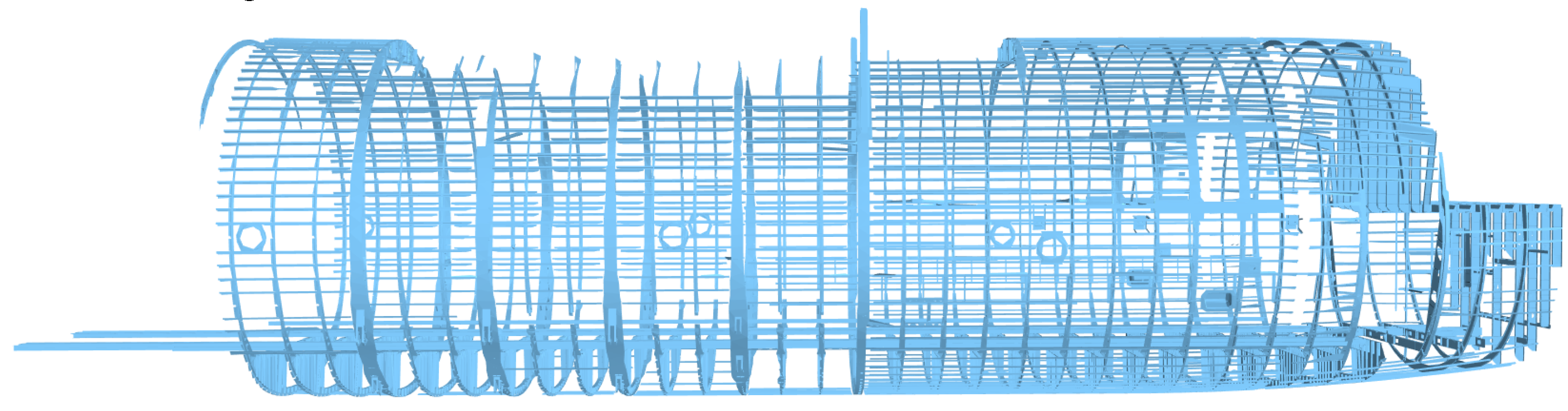
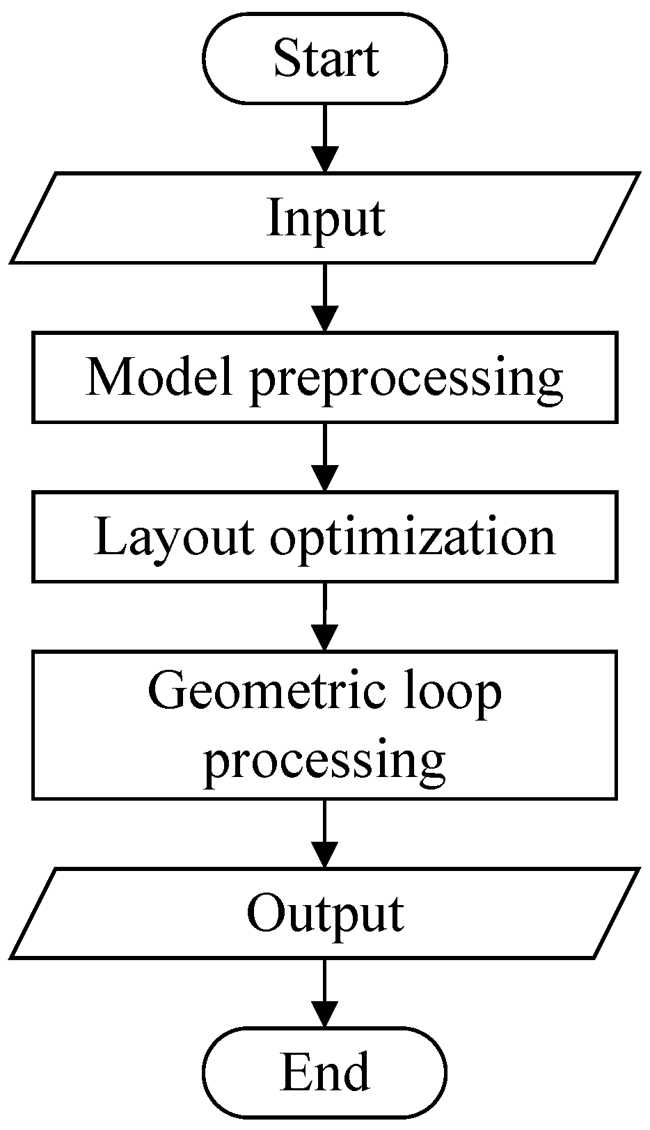
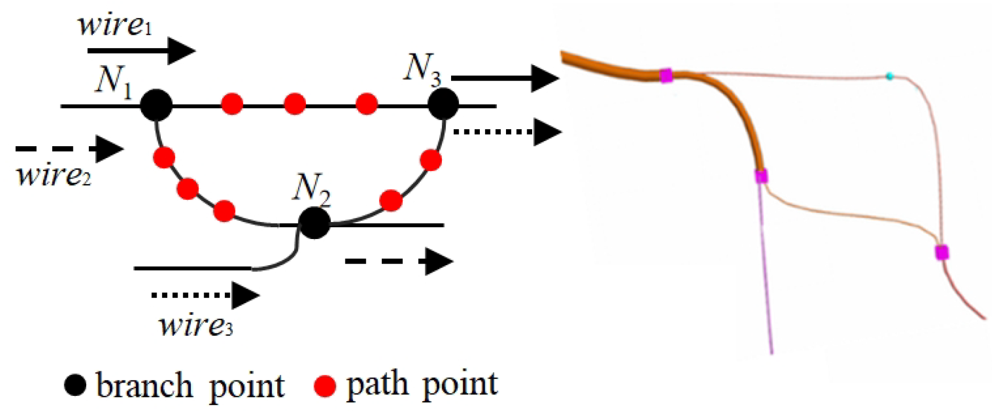
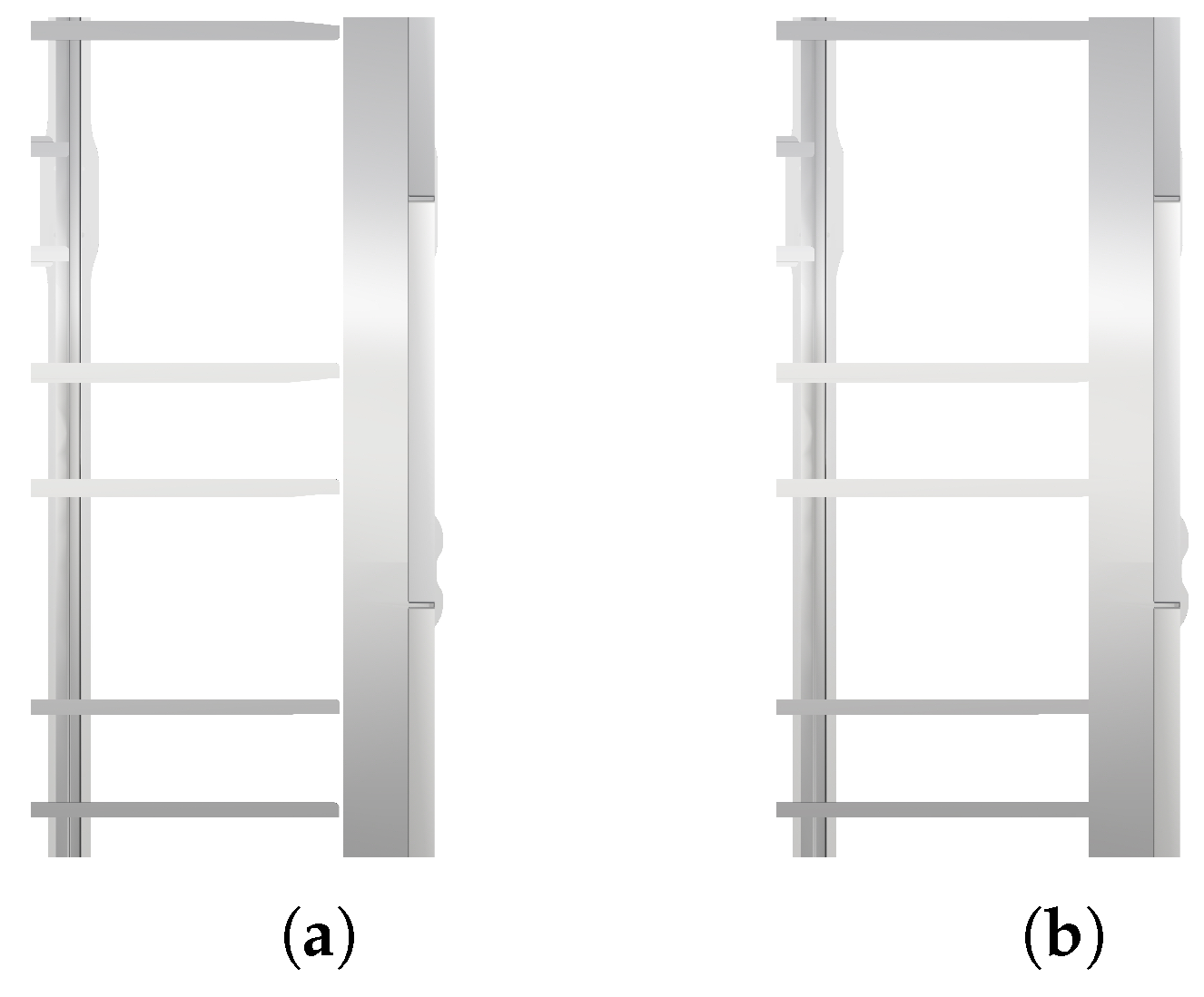
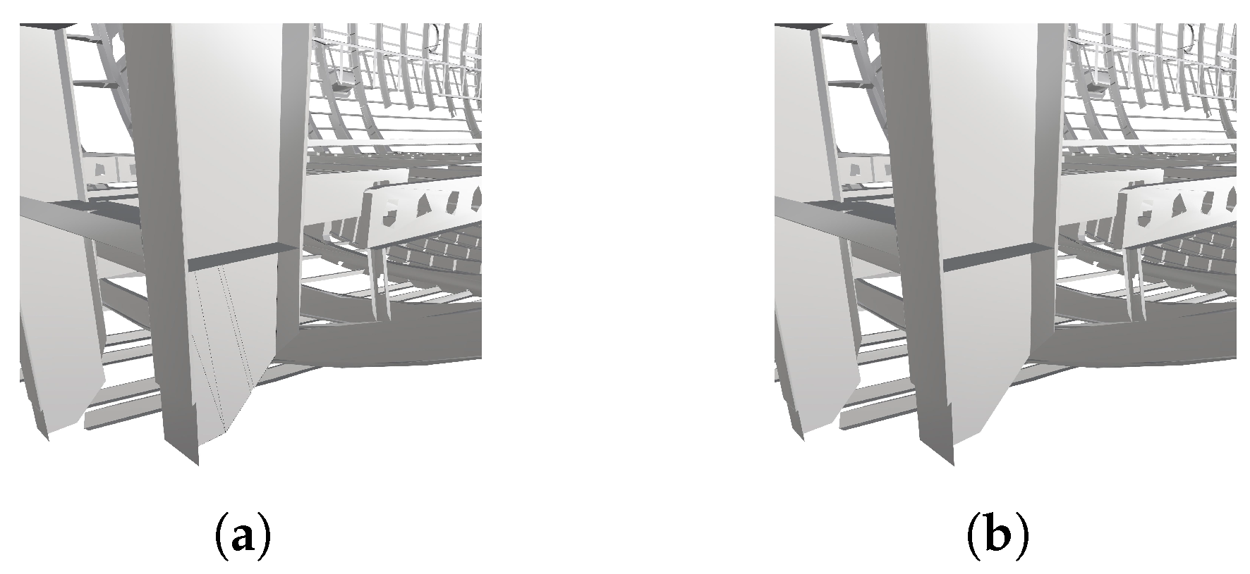
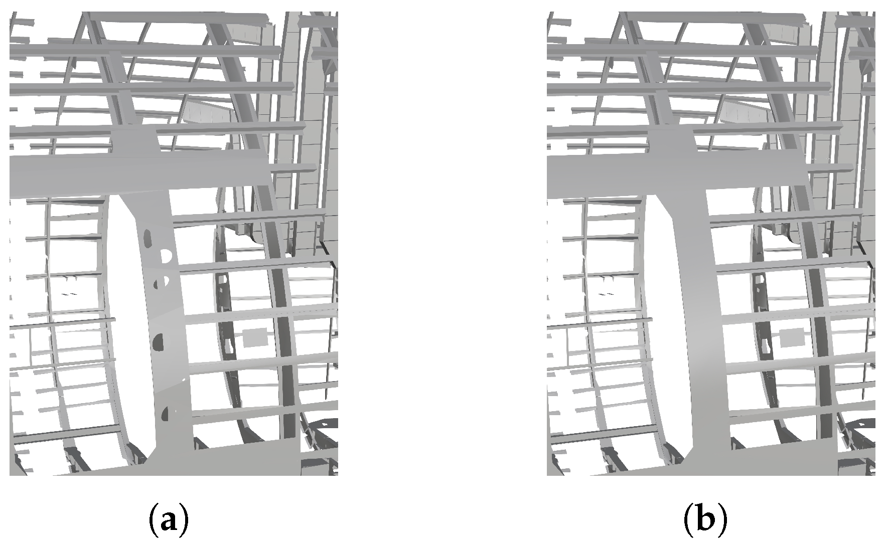


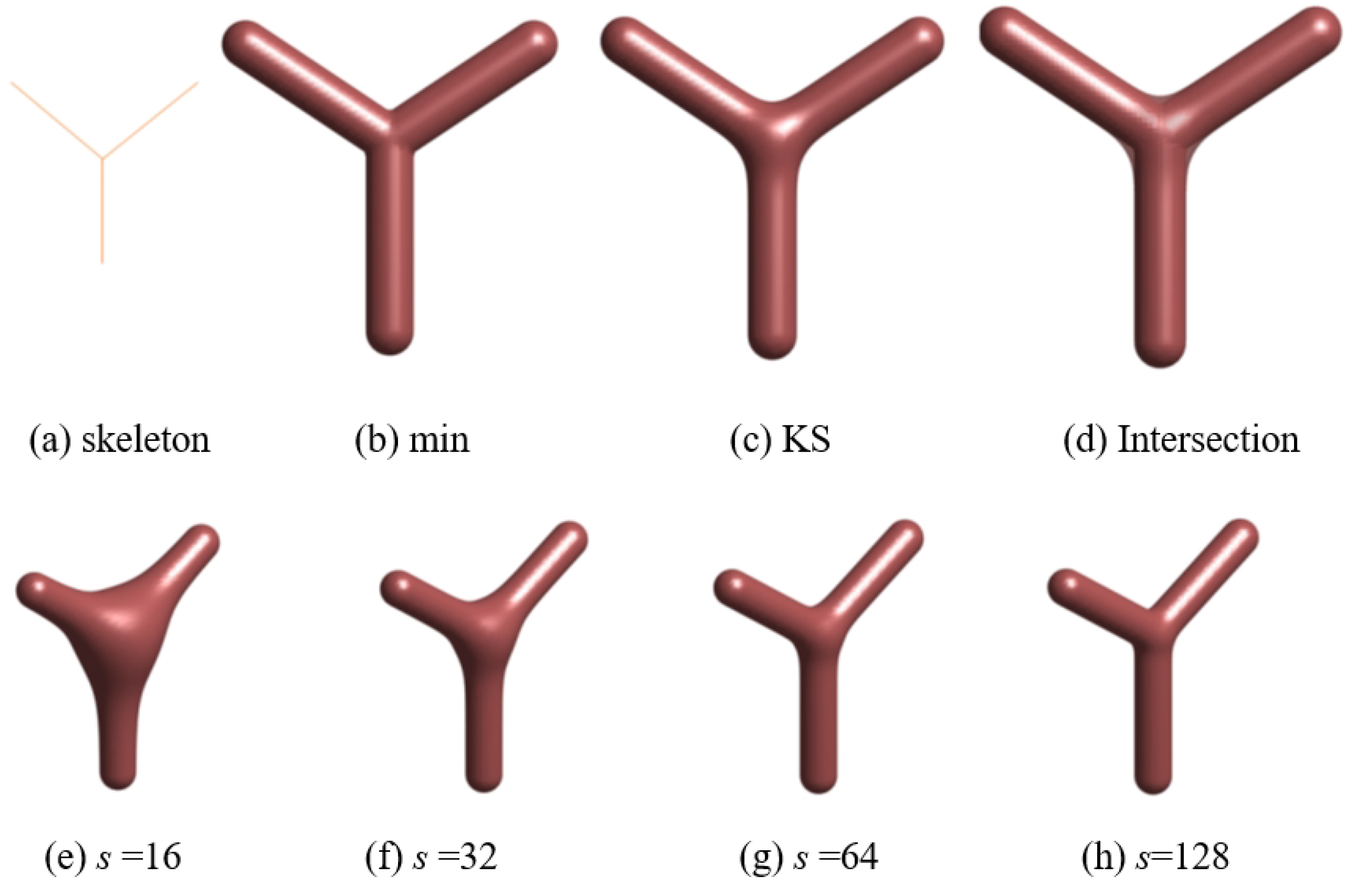
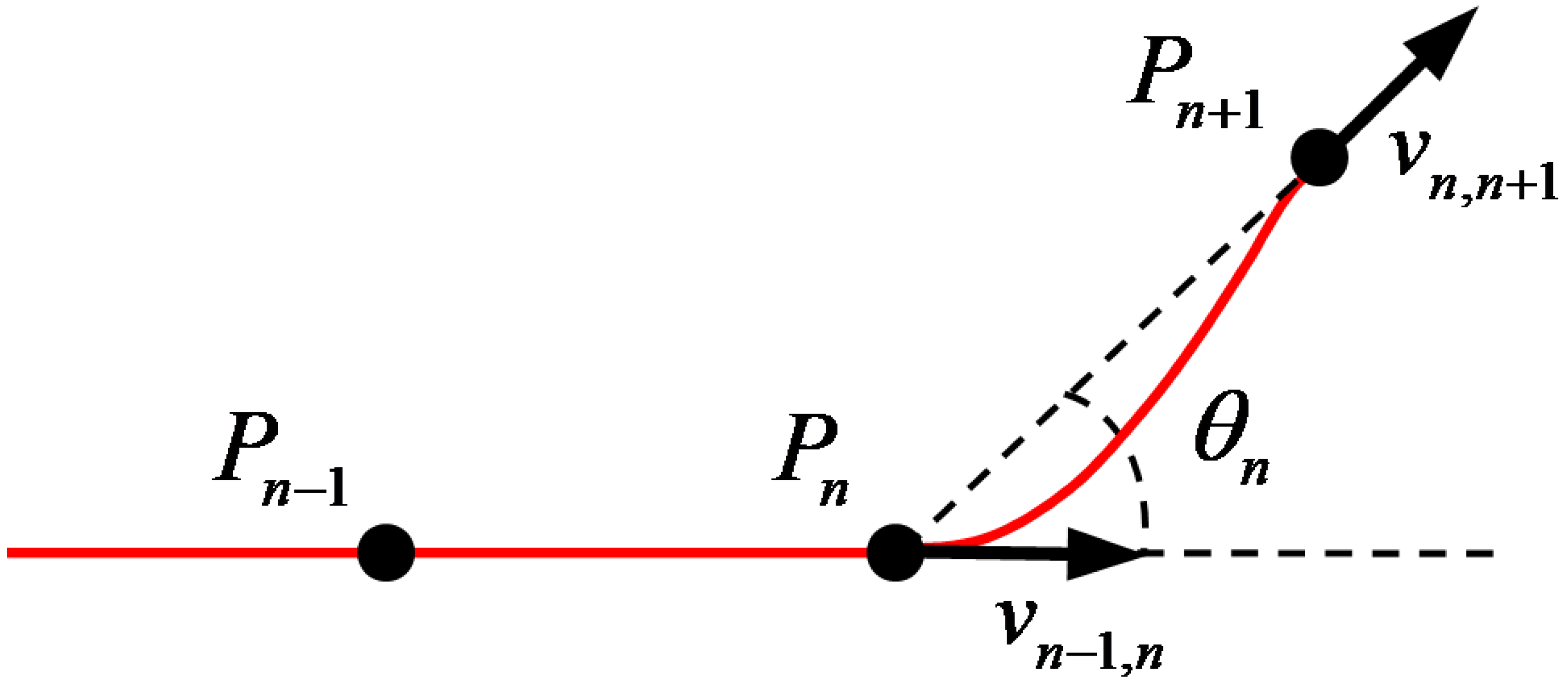


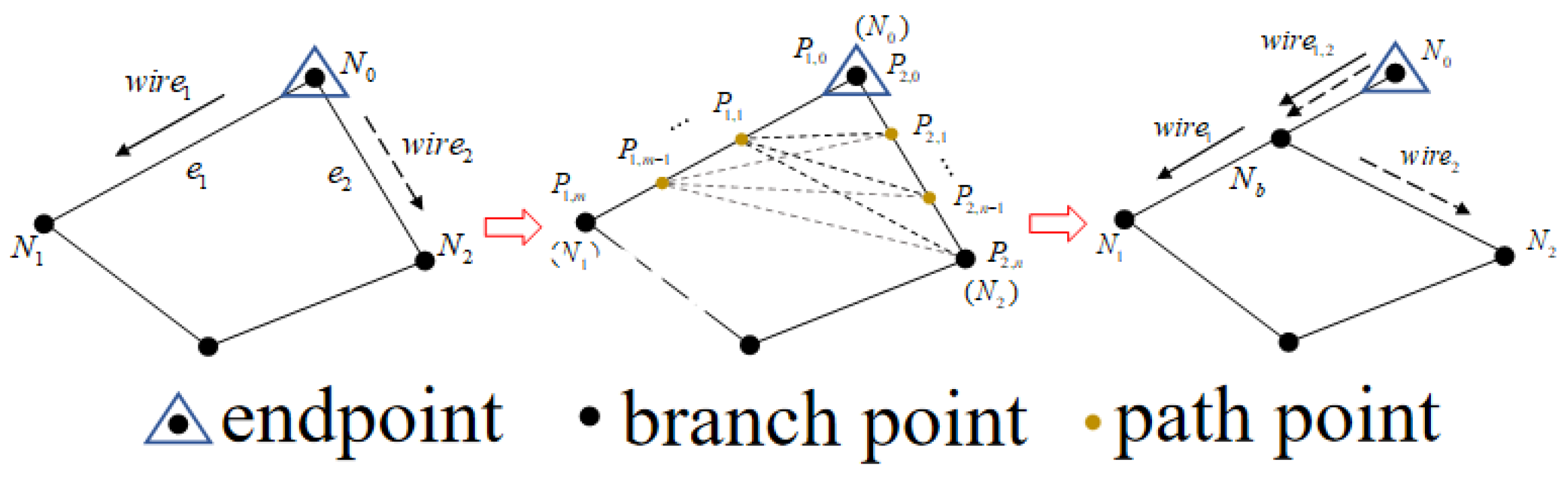
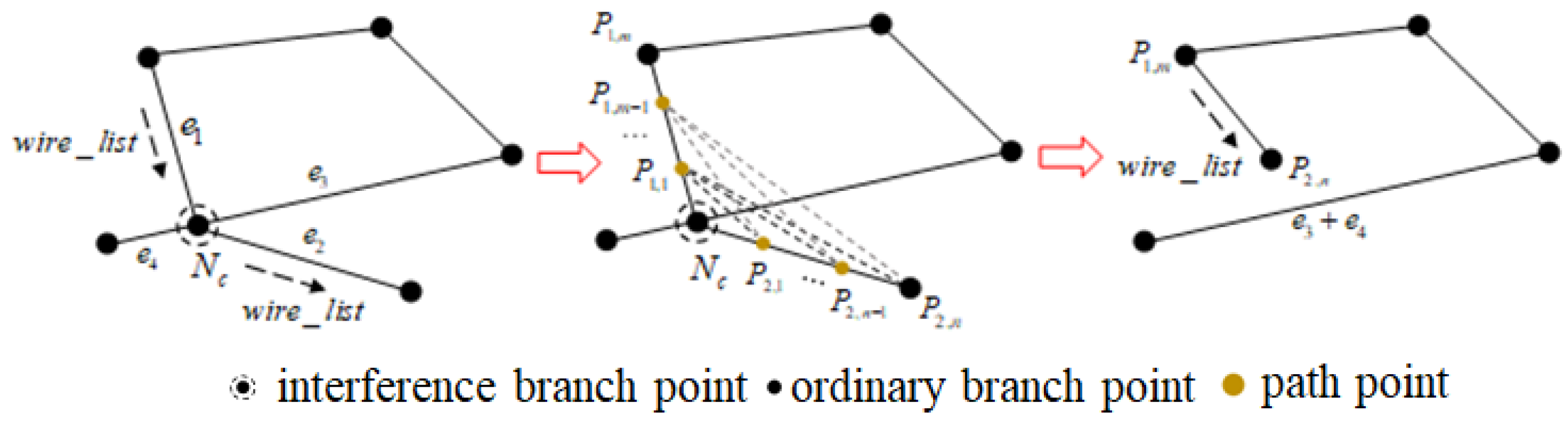

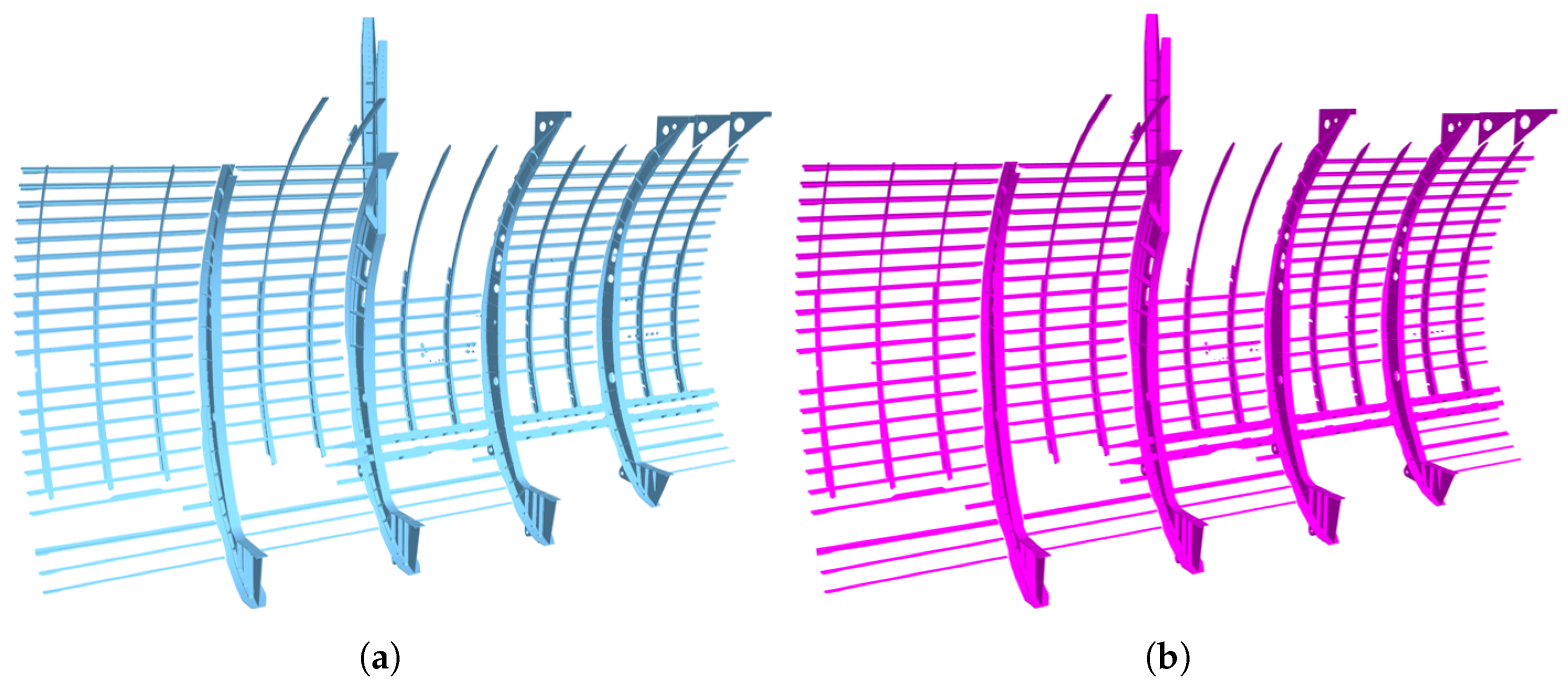


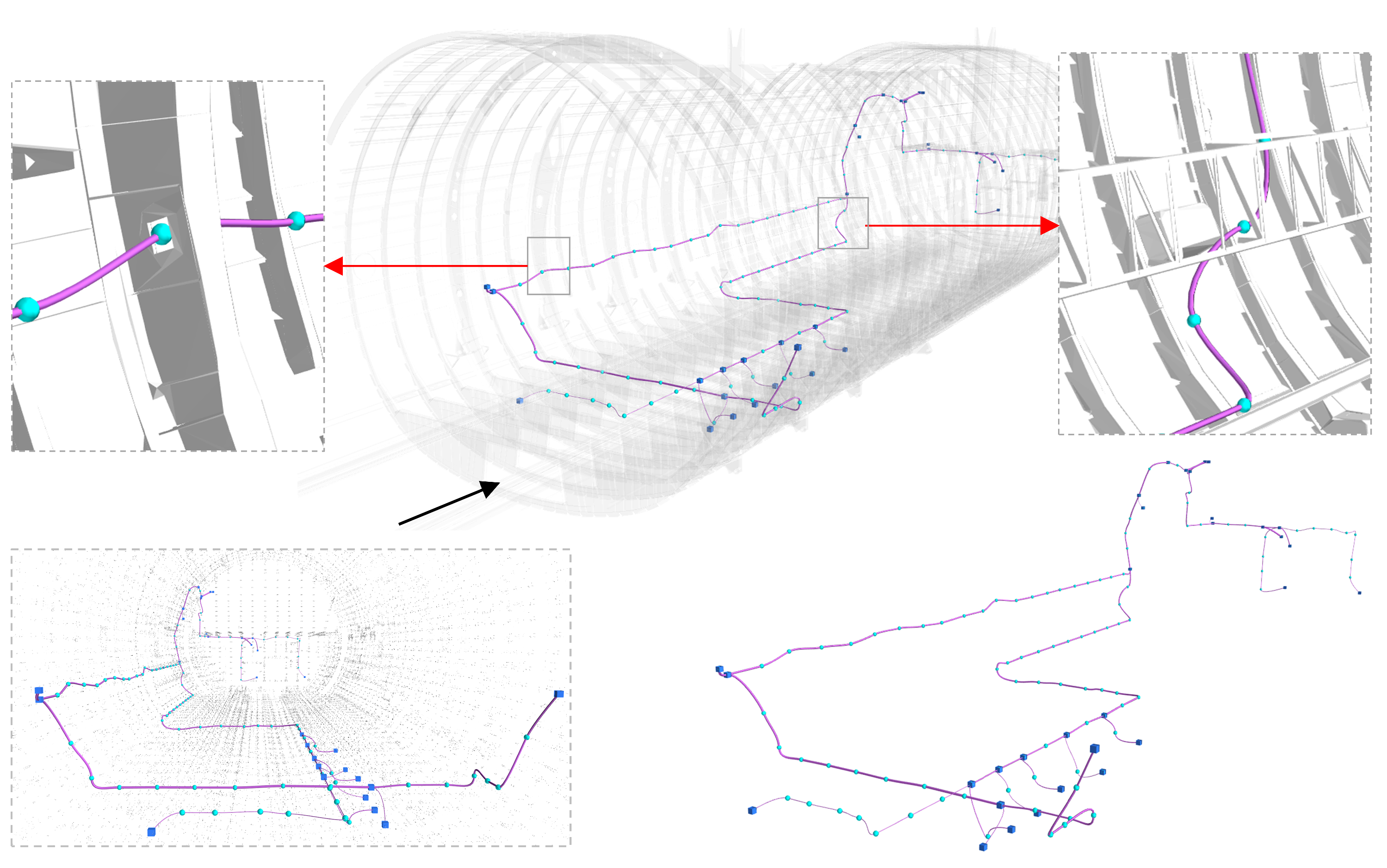

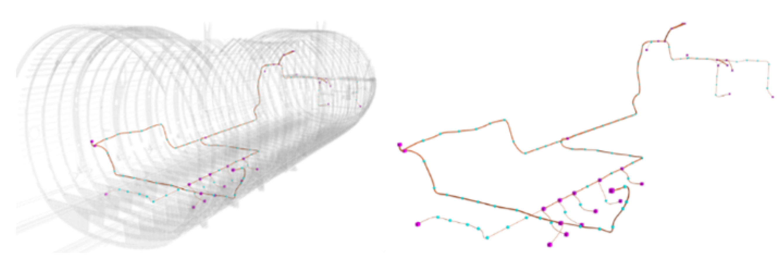
