Abstract
With the rapid advancement of technology, precision agriculture, as a modern agricultural production model, has seen significant progress in recent years. Its widespread adoption is gradually transforming traditional farming methods, providing strong support for the modernization of global agriculture. In particular, the application of positioning technology plays a crucial role in precision agriculture. This paper focuses on an automated agricultural machinery positioning system based on Bluetooth technology. The system uses Bluetooth at the 2.4 GHz frequency for transmission, processing Constant Tone Extension (CTE) and Received Signal Strength Indicator (RSSI) signals collected from blind nodes. The Propagator Direct Data Acquisition (PDDA) algorithm is employed to calculate angle information from CTE signals, while the Two-Ray Ground Reflection Model is applied to manage the correlation between RSSI and distance, making it suitable for outdoor environments. These two types of data are fused for positioning, with an optimized objective function converting the positioning task into an optimization problem. An Adaptive Secretary Bird Optimization Algorithm (ASBOA) is introduced to enhance the accuracy and efficiency of the positioning process. In the simulation, anchor and blind nodes are deployed to simulate a real farm environment. Anchor nodes receive CTE and RSSI signals from blind nodes. Considering that the tags mounted on agricultural machinery are set at a fixed height in real scenarios, the simulation also fixes the tags at this height. We then compare the accuracy of five algorithms in both static and dynamic tracking. The final simulation results indicate that ASBOA achieves satisfactory high-precision positioning, both for static points and dynamic tracking, theoretically meeting the needs for continuous positioning and laying a solid foundation for future field trials.
1. Introduction
Precision agriculture, as an innovative technology that integrates geospatial information, computer-aided decision-making, and agricultural engineering, has become a frontier trend in modern agricultural development and a key research focus. This technology, with its high technological content and strong comprehensive performance, significantly enhances the management of modern agriculture [1]. By applying precision agriculture, production efficiency and quality can be greatly improved. For instance, satellite positioning or IoT sensor technology allows for precise operations throughout the agricultural production process, such as targeted fertilization and yield forecasting [2]. The promotion of such technology not only enhances the precision of agricultural management but also facilitates the transformation of traditional agriculture into an efficient, refined, and high-yield modern agricultural model [3].
The modernization of the seed industry and agricultural mechanization represent the core directions of future agricultural development [4]. The adoption of intelligent and large-scale machinery has significantly boosted the efficiency and economic benefits of agricultural modernization and automation. However, automated agricultural machinery often requires complex operations, especially when driving [5]. Therefore, research into autonomous driving technologies for agricultural machinery is essential, as it can reduce operational complexity and mitigate the risks farmers face during pesticide application [6]. Examples of autonomous agricultural machinery are already present in modern agriculture, such as unmanned machines for planting, automated rotary tillers for land preparation, automated seeders, and automated sprayers for fertilization and pesticide application. Agricultural machinery in precision agriculture must be equipped with key functions such as positioning, planning, operation control, and monitoring to ensure efficient production [7]. As shown in Figure 1, the signals emitted by sensors on the automated machinery are received and processed by positioning stations to determine the machine’s location and plan its path.
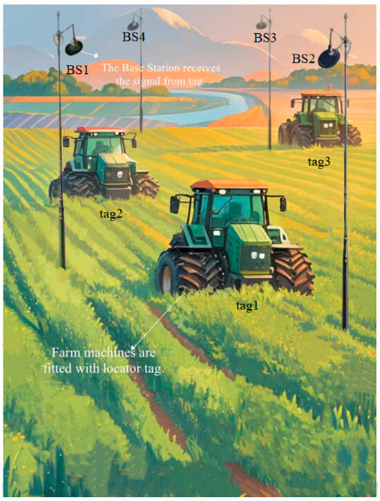
Figure 1.
Automated agricultural vehicle navigation and positioning diagram.
In outdoor applications, Bluetooth offers several significant advantages over GPS or other global positioning systems (such as GLONASS and Galileo) [8]. First, Bluetooth provides high positioning accuracy over short distances, typically achieving an accuracy of 1 m or even less. Second, Bluetooth’s low power consumption makes it ideal for devices that need to operate for extended periods with minimal energy usage. In contrast, GPS requires more power to maintain complex calculations and satellite connections. Bluetooth, on the other hand, can operate continuously at lower power, making it suitable for applications like drones and sensor networks. Additionally, Bluetooth devices are more cost-effective and flexible in deployment, making them suitable for large-scale applications, while GPS systems require higher deployment costs and more complex infrastructure. Furthermore, Bluetooth can operate within a closed, dedicated network, providing users with enhanced data security and privacy protection. Given these advantages, research on Bluetooth-based outdoor positioning is necessary.
BLE signal strength is generally regarded as an unreliable indicator for measuring proximity. Although numerous studies have focused on utilizing BLE signal strength and range in indoor settings, there remains a scarcity of research on outdoor systems. Nonetheless, BLE technology continues to advance, finding applications in various fields such as contact tracing, health monitoring, asset tracking, and proximity-based services or marketing [9].
Currently, low-power Bluetooth (BLE) positioning methods can be categorized into three main types as follows: (1) RSSI-based positioning, which is simple and cost-effective but prone to environmental interference and low accuracy; (2) angle-based positioning, including Angle of Arrival (AOA) and Angle of Departure (AOD), which determine position by measuring signal angles, offering high precision and being suitable for scenarios requiring accuracy; and (3) fingerprint-based positioning, which uses a prebuilt signal strength database, providing high accuracy but involving significant initial effort, high maintenance costs, and lower system stability. While some emerging methods exist, most are based on these three approaches.
In a previous study, Liu et al. point out that the positioning error of BLE-based systems under certain experimental conditions is approximately 1–2 m, which is consistent with our experimental results, further validating the reliability of our method [10]. Kong and Guo’s study shows that in open areas, BLE positioning accuracy can achieve within 3 m, which is in agreement with our findings and supports the effectiveness of BLE in such environments [11]. Additionally, Vasilenko and Schiller’s research found that the positioning error of BLE systems in outdoor environments generally ranges from 2 to 4 m, further confirming the feasibility of BLE technology for outdoor positioning [12].
For higher accuracy requirements, Li et al. proposed a BLE indoor positioning system where the positioning error remains stable at around 1 m in ideal conditions, demonstrating the potential of BLE technology for precise localization [13]. Moreover, Zhou and Zheng suggested that an improved BLE positioning method for outdoor applications can achieve positioning accuracy of approximately 1 m, further validating BLE’s effectiveness in high-precision positioning scenarios [14].
This study proposes a novel positioning method for outdoor precision agriculture. We select Bluetooth Low Energy (BLE) as the transmission technology, where anchor nodes receive CTE and RSSI signals from blind nodes. CTE signals are processed using the PDDA algorithm to calculate the Angle of Arrival (AOA) [15]. Considering the differences between typical indoor RSSI propagation models and those required for outdoor environments, we utilize the two-ray ground reflection model to manage RSSI signals [16]. By combining the relationship between RSSI and distance with angle information, a function is constructed to estimate the position. The positioning problem is framed as an optimization task, solved by minimizing the Euclidean distance between the actual and estimated positions. To address this optimization, we propose an Adaptive Secretary Bird Optimization Algorithm (ASBOA) and compare its positioning accuracy with several other algorithms under different scenarios.
The main objective of this study is to evaluate the effectiveness of the proposed method in a simulated environment. We designed a 2500 square meter simulation area to assess the positioning error under various conditions. This approach allows us to focus on the fundamental aspects of the positioning method and clearly demonstrate its feasibility and effectiveness in reducing errors. Our experimental results show that among the various algorithms, ASBOA has the smallest positioning error, achieving an average error of 0.47 m in static point positioning and the lowest 0.65 m in dynamic tracking positioning. The key contributions of this study are outlined as follows:
- (1)
- A positioning method is introduced, combining Angle of Arrival (AOA) and Received Signal Strength Indicator (RSSI), designed for outdoor agricultural machinery localization.
- (2)
- We introduce the Adaptive Secretary Bird Optimization Algorithm (ASBOA), which shows superior optimization performance compared to several other algorithms.
The rest of this paper is organized as follows: Section 2 elaborates on the selected positioning method and signal processing procedure. Section 3 will simulate the setting of simulation parameters and the process of mathematical modeling. Section 4 presents our proposed ASBOA algorithm and several comparison algorithms employed in the research. In Section 5, the algorithms are evaluated in two distinct scenarios, and the superiority of ASBOA is demonstrated. Finally, Section 6 summarizes the main conclusions of this study and offers recommendations for future research based on the limitations of this study.
2. Localization Method and Bluetooth Signal Processing
2.1. Localization Method
In this section, we introduce an outdoor localization method and propagation model based on Bluetooth Low Energy (BLE) technology [17]. BLE, a widely used short-range wireless communication standard, is compatible with most smartphones and computers. Its low power consumption and strong security features make it suitable for various indoor and outdoor applications. Typical BLE localization techniques involve methods such as RSSI, AOA, ToF, and fingerprinting [18].
RSSI-based localization calculates the distance between a target device and a base station by examining signal strength through a propagation model. To pinpoint the target’s location, trilateration is applied, relying on at least three reference points with known coordinates. This method provides a positioning accuracy of about 2 to 4 m [19].
ToF localization includes both Time of Arrival (ToA) and Time Difference of Arrival (TDoA) methods [20]. ToA calculates the distance by measuring the time it takes for the signal to travel between the BS and the target, followed by trilateration to pinpoint the location [21]. While this method is highly accurate, it requires precise clock synchronization, as any errors in timing can lead to inaccurate positioning. In contrast, TDoA measures the time difference of signal arrivals to calculate relative distances between the target and base stations [22]. TDoA also offers high localization precision, but synchronizing the clocks of multiple receivers is a key challenge [23].
The Angle of Arrival (AOA) method determines a target’s position by measuring the angle between the target and access points (APs), usually requiring more than two APs for accurate results. Fingerprint-based localization uses variations in RSSI across different locations to build a database of signal “fingerprints” at known positions. The user’s location is estimated by matching real-time RSSI readings with this database.
RSSI is commonly used in localization because of its simplicity and the way signal strength decreases with distance. However, its accuracy is generally limited. To address this, our study proposes a hybrid localization method that integrates AOA with RSSI to improve positioning accuracy and reliability.
2.2. Signal Processing
2.2.1. The Principle of BLE AOA
In 2019, the Bluetooth Special Interest Group (SIG) introduced the Bluetooth 5.1 standard [24]. Compared to Bluetooth 5.0, this version includes a direction-finding capability that enables angle measurements for AOA (Angle of Arrival) and AOD (Angle of Departure). This is achieved by receiving Bluetooth signals with an antenna array, allowing for more precise positioning. Using the AOA method, the receiving device can determine the angle of the signal arriving from a single transmitter. In contrast, the AOD method enables the receiving device to estimate its location by capturing signals from multiple transmitters. As shown in Figure 2, Bluetooth AOA technology measures the signal’s incidence angle through an antenna array. Overall, the changes in version 5.1 mean that the transmitter uses a single antenna to send Bluetooth data packets with direction-finding capability, while the receiver captures signals using multiple antennas.
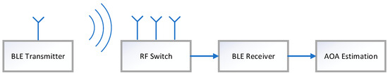
Figure 2.
Architecture of the BLE AOA system.
The Bluetooth 5.1 specification defines the CTE standard, where the CTE signal consists of a sequence of unwhitened 1 s. This signal is transmitted long enough for IQ values to be received without impacting the receiver’s modulation. Here, I represents the in-phase component of the signal, while Q represents the quadrature component. Due to the widespread use of low-power Bluetooth standards, many indoor positioning systems have already incorporated AOA technology. Although CTE is a brief continuous wave lasting between 16 μs and 160 μs, it is divided into multiple segments according to the Bluetooth 5.1 core specification, as shown in Figure 3.
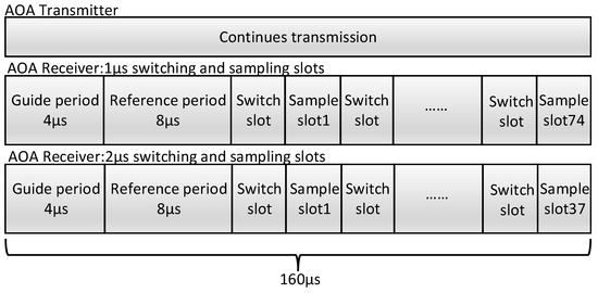
Figure 3.
Constant Tone Extension structure.
BLE uses the 2FSK modulation as shown in Equation (1) as follows:
where represents the modulated signal. The carrier frequency is denoted by , and stands for frequency deviation. When bit 1 is modulated, the frequency becomes , whereas for bit 0, it shifts to . The initial phases are represented by and . In AOA systems, is .
As the signal reaches the antenna array, a phase difference arises between the antennas, which is subsequently utilized to determine the signal’s angle of arrival (AOA).
- (1)
- Linear Antenna Array Received Signal Model:
Figure 4 shows a model of a linear antenna array. As CTE is a sinusoidal wave, it exemplifies a standard narrowband signal. Assuming the transmitter operates in the far-field region, the array consists of antennas, with a spacing of between each neighboring antenna.
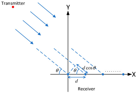
Figure 4.
Linear antenna array received signal model.
- (2)
- PDDA: The PDDA algorithm determines AOA by utilizing the received signal instead of the covariance matrix. It calculates the propagation vector , which defines the relationship between the signal at the first antenna (first row) and the other antennas (subsequent rows) [25]. By normalizing this vector to the first element, it eliminates the dependency on the signal’s time series. As a result, the propagation vector preserves comprehensive information on how signal phases from various directions combine at each antenna. The core concept of the PDDA algorithm is as follows:
The received CTE signal, after processing, can be expressed as Equation (2) as follows:
To calculate the propagation vector , we choose to divide the matrix into Equations (3) and (4) as follows:
Next, the propagation vector is defined to represent the cross-correlation between the signal at the first antenna and those at the other antennas. This vector illustrates the phase shift of the signal across the antenna array, representing it through the cumulative phases at each antenna. By normalizing the phase of its initial element, any dependency on the time series of the signal is eliminated, ensuring time does not impact subsequent calculations. The definition of vector is shown in Equation (5) as follows:
The 1 × M vector is formed by adding a unit element to represent the correlation of the first row with itself as Equation (6) as follows:
This allows us to derive the expression for the angle of the maximum peak in the AOA as Equation (7) as follows:
where represents the steering vector, given by Equation (8) as follows:
2.2.2. RSSI Propagation Model
In outdoor positioning scenarios, due to the open environment, the commonly used log-normal model is not suitable. Instead, the two-ray ground reflection model is required because it better captures the impact of ground reflections on signal propagation in outdoor environments. Since the target positioning system is designed for automated agricultural machines operating in open farmlands, the effect of ground reflection on signal strength is significant. The free space model does not account for this impact, while the tree path loss model is more suited for densely vegetated or forested areas. Although these models may offer different perspectives, the two-ray ground reflection model provides a more accurate representation of the conditions in agricultural environments.
This model is frequently employed in wireless communications, taking into account both the direct path and the ground-reflected path. According to this model, signals between the transmitting and receiving antennas travel via two paths: a direct path and a path reflected by the ground, as illustrated in Figure 5. A key challenge of the two-ray ground reflection model lies in the fact that the relationship between RSSI and distance is not uniquely defined, unlike in the log-normal model. This means that although the model can map distance to RSSI values, a single RSSI measurement might correspond to several different distances, as illustrated in Figure 6.
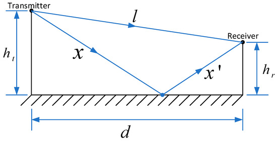
Figure 5.
Two-ray ground-reflection model.
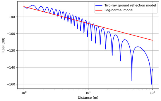
Figure 6.
Propagation of log-normal model and two-ray reflection model.
Using the two-ray ground-reflection model makes it much harder to determine target position coordinates from RSSI, posing a significant challenge in conventional positioning methods.
3. Modeling Simulation
In this section, we introduce the environmental model and objective function. The anchor node receives signals from the blind node, including RSSI, vertical Angle of Arrival (AOA), and horizontal AOA. In an outdoor environment, based on the RSSI reflection model, a single RSSI value can correspond to multiple distances, making it challenging to obtain an accurate distance with RSSI alone. By incorporating angle information, estimated coordinates are derived. The Euclidean distance between the actual and estimated coordinates is then used as the objective function, and optimization algorithms are applied to minimize this difference, filtering out distances that do not match the actual RSSI value. The point at which the minimized value occurs represents the estimated actual coordinates.
We used the Numpy library to generate the coordinates of the locators and tags within the specified range. The PyBLE library was employed to simulate the signal transmission between BLE tags and locators. Each tag sends out RSSI and CTE signals. The received RSSI signals are transmitted using the two-ray ground reflection model, while the received CTE signals are processed using the PDDA algorithm.
3.1. Modeling Parameters
In this study, we set the simulation area to 2500 square meters and arranged 16 anchor nodes, each with a height of 6 m. For outdoor use, we selected the 2.4 GHz frequency due to its greater transmission range compared to 5 GHz. The blind nodes were positioned at a height of 1.5 m. The environmental conditions are provided in Table 1, while Figure 7 displays the layout of the simulation zone and the positioning of the surrounding anchor nodes.

Table 1.
Modeling parameters.
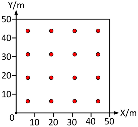
Figure 7.
Anchor node distribution on the h = 6 m plane.
3.2. Modeling of Localization Problems
According to the arrangement of the anchor nodes described above, the RSSI value measured by each anchor node is denoted as , the horizontal angle of arrival is denoted as , and the vertical angle of arrival is denoted as , where ranges from 1 to , with indicating the total count of anchor nodes.
According to the two-ray ground-reflection model, the correlation between RSSI and distance can be expressed as Equation (9) as follows:
where is the transmitted power, is the gain at the transmitter, is the gain at the transmitter, is the wavelength, is the height of the transmitter, is the height of the receiver, and is the distance between the transmitter and th receiver. As mentioned, in Formula (9), the same RSSI value may correspond to multiple distances d. However, by incorporating angle information, those distances that do not correctly reflect the actual distance can be excluded. Therefore, it is feasible to use this model for simulation.
The horizontal angle of arrival and the vertical angle of arrival provide information about the direction of the signal’s arrival. Let the position of the anchor node be and the position of the blind node be . The relative position between the two can be given by Equation (10) as follows:
Combining the above RSSI and AOA information, the Euclidean distance from the blind node to each anchor node can be determined. For convenience, the squared distance is used in Equation (11) as follows:
Since the height of the blind node is fixed, therefore . This function represents the difference between the actual measurements and the model predictions. A smaller target value indicates a closer proximity to the target node.
In our simulations, Python 3.7 is utilized to implement the two-ray ground reflection model and to configure angle-of-arrival (AOA) antennas, enabling the simulation of signal transmission and the generation of measured RSSI and AOA values. The overall simulation flowchart is shown in Figure 8.
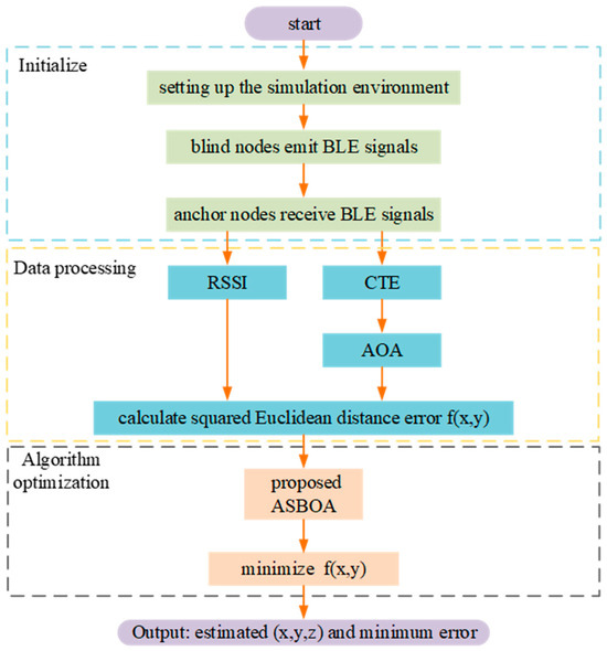
Figure 8.
Simulation experiment flowchart.
4. Introduction to Optimization Algorithms
In this section, we introduce the algorithms used in this study. As outlined in the previous chapter, the localization problem has been reframed as an optimization task. A range of traditional algorithms, such as Simulated Annealing (SA), Genetic Algorithm (GA), Gradient Descent (GD), and Particle Swarm Optimization (PSO), can address this type of problem. However, due to the complexity of the problem, simpler and widely used algorithms often tend to converge to local rather than global optima. Therefore, we proposed the Adaptive Secretary Bird Optimization Algorithm (ASBOA). In this study, we employ several optimization algorithms, including GD, SA, PSO, the Secretary Bird Optimization Algorithm (SBOA), and the ASBOA.
4.1. Secretary Bird Optimization Algorithm
SBOA is a heuristic optimization algorithm inspired by the hunting behavior of the African Secretary Bird [26]. Known for its unique hunting methods and efficient search strategies, this algorithm aims to mimic these behaviors to solve complex optimization problems. SBOA effectively searches for the optimal solution in the search space by simulating the Secretary Bird’s ground searching, rapid running, and precise striking behaviors. The basic steps of SBOA are as follows:
- (1)
- Algorithm initialization phase: The positions of the bird group are first initialized by randomly generating each secretary bird’s position within the defined search space. Each position is then designated as a candidate solution, and the objective function value for each candidate is calculated and stored in a vector for subsequent optimal solution selection. The process of randomly initializing the birds’ positions within the search space is illustrated by Equation (12). These potential solutions are randomly generated under the constraints of the upper and lower bounds of the given problem, and the best solution obtained at this stage is tentatively considered the optimal solution for each iteration. The population of candidate solutions is depicted by Equation (13).
In this context, each secretary bird symbolizes a potential solution for optimizing the problem. Consequently, the objective function is assessed based on the values suggested by each secretary bird for the problem’s variables. The calculated values of the objective function are then assembled into a vector as outlined in Equation (14).
In this framework, F denotes the vector containing objective function values, where represents the objective function value associated with the i-th secretary bird. By comparing these values, the quality of each candidate solution is effectively evaluated, helping to identify the optimal solution for the given problem. As the positions of the secretary birds and the objective function values are revised in every iteration, it becomes essential to identify the best candidate solution in each cycle as well.
- (2)
- Exploration phase: The hunting behavior of secretary birds when preying on snakes is generally broken down into three distinct steps: searching for prey, consuming prey, and attacking prey. In SBOA, each of these stages is modeled as follows:
Step 1: This phase utilizes a differential evolution approach, which leverages differences among individuals to create new solutions, thus boosting both algorithm diversity and global search potential. By incorporating differential mutation processes, diversity aids in preventing the algorithm from becoming confined to local optima. Individuals can explore various areas within the solution space, enhancing the likelihood of reaching the global optimum. Consequently, the position update for the secretary bird in the Locating Prey phase can be expressed mathematically using Equations (15) and (16).
where indicates the current iteration number, denotes the total number of iterations, and represents the updated state of the i-th secretary bird in the first step. Meanwhile, and are randomly selected candidate solutions during this stage. Additionally, refers to a randomly generated array of size 1 × within the range [0, 1], with Dim representing the dimensionality of the solution space. Finally, specifies the value in the -th dimension, and indicates its objective function fitness value.
Step 2: In this phase, Brownian motion (RB) is introduced to simulate the secretary bird’s random movements. Mathematically modeled by Equation (17), Brownian motion allows the secretary bird to occasionally pause and lock onto the snake’s location using its sharp vision. We apply the concept of (the individual’s historically best position) in combination with Brownian motion, allowing individuals to conduct local searches toward their previously identified best positions, thereby enhancing exploration within the surrounding solution space. This approach not only prevents individuals from prematurely converging to local optima but also accelerates the algorithm’s progression toward optimal positions in the solution space. By enabling searches based on both global information and each individual’s historical best, the chances of locating the global optimum are increased. Introducing Brownian motion’s randomness further improves exploration effectiveness, helping individuals avoid local optima and achieve better outcomes in tackling complex problems. Consequently, the position update of the secretary bird in the Consuming Prey phase can be modeled mathematically using Equations (18) and (19).
where denotes an array generated randomly with dimensions , drawn from a standard normal distribution (mean of 0 and standard deviation of 1). Meanwhile, refers to the current best value found.
Step 3: In the process of random search, introducing the Lévy flight strategy strengthens the optimizer’s global search capabilities, reduces the likelihood of SBOA getting stuck in local solutions, and enhances the algorithm’s convergence precision. By simulating the flight abilities of the secretary bird, search space exploration is further expanded. Large steps allow the algorithm to cover the search space more broadly, enabling individuals to reach the optimal position faster, while smaller steps improve the precision of optimization. To make SBOA more dynamic, adaptive, and flexible during optimization—achieving a more balanced trade-off between exploration and exploitation, avoiding early convergence, accelerating overall convergence, and enhancing algorithm performance—a nonlinear perturbation factor has been added. Consequently, the update of the secretary bird’s position during the prey attack phase can be mathematically represented through Equations (20) and (21).
To improve the algorithm’s optimization accuracy, we apply a weighted Lévy flight, which is represented as in Equation (22).
- (3)
- Exploitation phase: The secretary bird generally employs two main evasion strategies to protect itself or its food. The first is rapid running or flying, and the second is camouflage, where the bird blends into its surroundings using colors or structures in the environment to evade predators. Assume that one of these two scenarios occurs with the same probability:
: Blending into the surroundings.
: Escape by running or flying.
When the secretary bird detects a predator nearby, it first seeks a suitable place for camouflage. If no safe and appropriate camouflage environment is available, it chooses to escape by flying or running quickly. In this context, we introduce a dynamic perturbation factor, which aids the algorithm in balancing exploration and exploitation. Adjusting these factors allows for increased exploration or strengthened exploitation at various stages. To summarize, the secretary bird’s two evasion strategies are mathematically modeled by Equation (23), with the updated conditions described by Equation (24).
where is assigned a value of 0.5, denotes an array randomly generated following a normal distribution, represents the random candidate solution for the current iteration, and indicates a randomly selected integer, which is either 1 or 2.
4.2. Adaptive Secretary Bird Optimization Algorithm
Based on SBOA, this study proposes ASBOA (Adaptive Secretary Bird Optimization Algorithm), which improves on several shortcomings of SBOA as follows:
- (1)
- Adaptive Parameter Adjustment: The current algorithm uses a fixed step size at each stage. By setting the step size as adaptive, larger steps are allowed during the early exploration phase, while smaller steps can refine the search in later stages. Additionally, linking the weights of Brownian motion and Lévy flight to the iteration count allows their contributions to adjust dynamically over time.
- (2)
- Increasing Diversity to Prevent Early Convergence: Randomly selecting different update strategies at each stage enhances individual diversity.
- (3)
- Introducing a Memory Mechanism: Recording the current optimal solution prevents the best solution from being lost during mutation and crossover operations.
- (4)
- Using Clustering for Initialization: This approach forms a well-distributed starting population.
With these improvements, ASBOA becomes more adaptable in handling various optimization problems, enhancing both global search and local exploitation efficiency, which leads to better solutions in complex optimization tasks.
The specific steps of the ASBOA algorithm are as follows and the flowchart is shown in Figure 9:
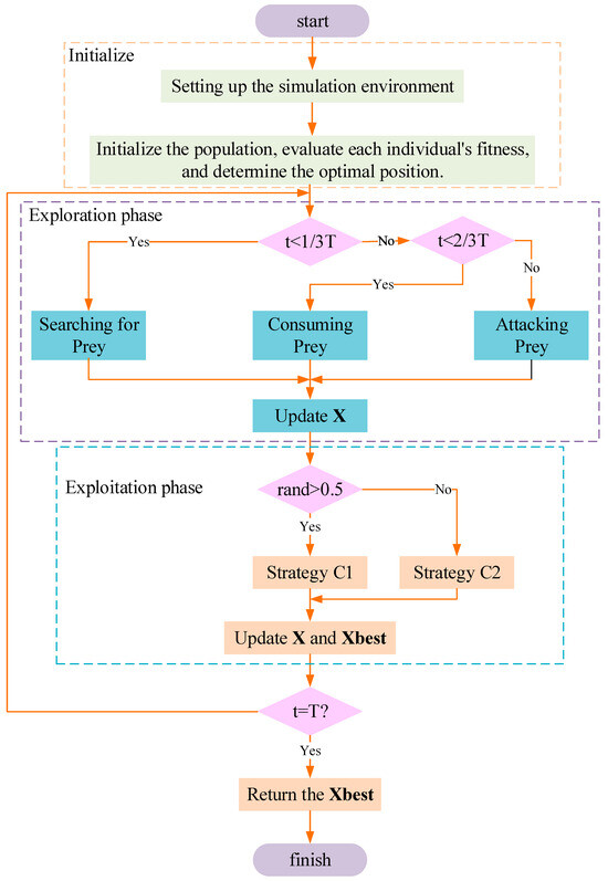
Figure 9.
The flowchart of ASBOA.
- (1)
- Initialization Phase: First, set the dimension of the problem, population size N, maximum iteration number T, and the bounds and . Second, randomly generate a group within the search space, using the -means algorithm to divide these solutions into clusters, and use the cluster centers as the initial solutions in Equation (25).
- (2)
- Dynamic Step Size Adjustment: Adjust the step size dynamically in each iteration to balance exploration and exploitation as follows in Equation (26).
Adaptive Weights for Brownian Motion and Lévy Flight: Dynamically adjust the weights of Brownian motion and Lévy flight based on the iteration count in Equation (27).
Update Equation: Update the position using the adaptive step size and weights in Equation (28).
- (3)
- Exploration Phase: In the exploration phase, we introduce a mixed strategy, randomly selecting crossover and mutation strategies to increase population diversity.
The crossover operation refers to randomly generating another solution, with the new position given by Equation (29) as follows:
where is a random coefficient used to control the fusion ratio of the two solutions.
The mutation operation refers to mutating the solution, as given by Equation (30).
Here, represents the mutation step size.
- (4)
- Memory Mechanism: In each iteration, we consider retaining the global best solution while also saving and synchronizing each individual’s historical best solution. The specific steps are as follows: after each iteration, record the current optimal solution. If a new solution outperforms the historical best, update the position of the historical best solution. Each individual also retains its own historical best solution, using it to guide its movement. The specific update formula is as follows in Equations (31) and (32):
4.3. Gradient Descent Algorithm
Gradient Descent (GD) is a commonly used optimization algorithm, widely applied in machine learning and deep learning to minimize loss functions [27]. The core concept involves repeatedly adjusting parameters by following the direction opposite to the gradient of the loss function, which incrementally brings the model closer to the function’s minimum. The basic steps of GD are as follows:
- (1)
- Initialization: Give an initial point to start in the search space.
- (2)
- Iterative update: In each iteration, adjust the position in the direction that opposes the gradient of the objective function according to Equation (33) as follows:
This process continues until either a specified number of iterations has been performed or a target objective value is reached.
4.4. Simulated Annealing Algorithm
Simulated Annealing (SA) was independently introduced by multiple researchers. It is a metaheuristic stochastic optimization algorithm inspired by the physical process of annealing in metals. During the metal annealing process, materials are slowly cooled from a high temperature to reach their lowest energy state. By mimicking this process, the SA algorithm aims to find the global optimum for complex optimization problems. The approach begins with a relatively high initial temperature, and, as the temperature gradually decreases, it searches for the global optimum in the solution space through random sampling. The annealing process begins with an initial solution . During each iteration, a new solution is produced within the neighborhood of the current one. The key steps of Simulated Annealing are outlined as follows:
- (1)
- Energy Difference: Starting from the current solution , generate a new solution through a certain perturbation mechanism. Calculate the difference in energy between the new and old solutions as Equation (34) as follows:
- (2)
- Acceptance Criteria: The acceptance or rejection of a new solution is determined by two primary conditions. If the new solution is better than the current solution (), it is accepted directly. If the new solution is worse (), it is accepted with a probability that depends on the current temperature. This probability is calculated using Equation (35) as follows:
- (3)
- Temperature Dispatch: At the start of the algorithm, a high temperature promotes a broad search, allowing even poor solutions to be accepted. As time progresses, the temperature gradually decreases, reducing the likelihood of accepting low-quality solutions. The temperature schedule is determined by Equation (36) as follows:
- (4)
- Termination Conditions: The algorithm terminates and returns the current best solution once the temperature is reduced to a predetermined threshold or it reaches a predefined maximum number of iterations.
4.5. Particle Swarm Optimization Algorithm
Particle Swarm Optimization (PSO) is an algorithm rooted in swarm intelligence, initially introduced by Kennedy and Eberhart [28]. It draws inspiration from the collective behavior of birds and fish. PSO simulates the movement of particles through the search space to gradually converge on the best solution. The main steps of the PSO algorithm are as follows:
- (1)
- Initialize particles: Randomly generate a set of particle positions and velocities. Initialize optimal solutions: Calculate each particle’s fitness, and initialize the personal best () and global best ().
- (2)
- Fitness evaluation: Evaluate the fitness of each particle by calculating the objective function .
- (3)
- Update personal and global best: Each particle keeps track of its personal best position () and the global best position () for the entire swarm.
- (4)
- Update rule: In each iteration, adjust the velocity and position of each particle according to the update rules by Equations (37) and (38) as follows:
These steps are repeated until a set number of iterations is completed or another stopping condition is satisfied. The optimal solution from the last iteration is then regarded as the solution to the optimization problem.
5. Evaluation
In this section, we evaluate the proposed positioning method. First, we assess the performance of the algorithm when dealing with random static points in the selected area. Then, we generate three random dynamic points for localization. Since actual movement is continuous, we restrict the search space to the neighborhood of the previous point. Finally, we discuss the overall results and trends.
5.1. Random Position
We randomly generated 50 positions within a 50 m × 50 m range. Each algorithm was run 50 times at each position. Statistical analysis was performed based on the obtained results, with the error distribution of each algorithm shown in Figure 10.
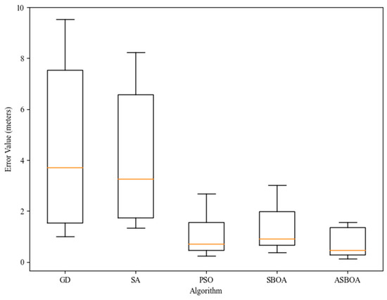
Figure 10.
Error values of different algorithms in random positions.
Different algorithms exhibited significant differences in positioning accuracy. The Adaptive Bat Optimization Algorithm (ASBOA) had the smallest average error of 0.47 m, indicating its high average positioning precision. Its maximum error was 1.56 m, suggesting relatively stable performance even in worst-case scenarios. Particle Swarm Optimization (PSO) showed a slightly higher average error of 0.72 m, but its maximum error reached 2.68 m, indicating potential large deviations under certain circumstances. The Bat Optimization Algorithm (SBOA) had an average error of 0.91 m and a maximum error of 3.01 m. Additionally, Gradient Descent (GD) and Simulated Annealing (SA) reported average errors of 2.72 m and 3.15 m, respectively, showing poorer overall performance compared to the first three algorithms. Notably, GD had a maximum error of 9.53 m, and SA had a maximum error of 8.24 m, highlighting the possibility of significant positioning errors under specific conditions. Besides the maximum and average errors, the minimum errors for ASBOA, SBOA, and PSO were all within 0.5 m, specifically 0.13 m, 0.37 m, and 0.24 m, respectively. In contrast, the minimum errors for GD and SA were both above 1 m, reflecting less ideal optimization capabilities of these two algorithms in this scenario.
In summary, ASBOA, PSO, and SBOA outperformed the other algorithms. Particularly, ASBOA excelled in both average precision and stability. By comparison, SA and GD performed poorly. Therefore, in subsequent evaluations, we will no longer consider SA and GD.
To assess the effectiveness of various algorithms across different domains, we divide the entire region into 100 sub-regions, each with a size of 5 m × 5 m. In each sub-region, we generate 10 position coordinates. We then run each algorithm at these points and calculate the average error for each sub-region. The results are shown in Figure 11.
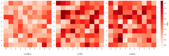
Figure 11.
Average error of 4 algorithms in each subarea.
The average error of the Particle Swarm Optimization (PSO) algorithm is 1.48 m, indicating that the overall error is within a controllable range. The standard deviation is 1.73, suggesting some fluctuation in the error distribution. In comparison, the ASBOA algorithm achieves the lowest average error of 1.05 m, demonstrating the best overall performance among the three algorithms. Its standard deviation of 0.91 is relatively small, indicating high consistency in the results. The maximum error for ASBOA is 3.07 m, also the smallest among the three algorithms, which suggests that the algorithm performs well even in extreme cases.
The SBOA algorithm has a higher average error of 1.95 m, which is worse than that of PSO, indicating its relatively poorer overall performance. The maximum error of 4.22 m is also relatively high, suggesting that the algorithm may exhibit instability in certain regions. However, SBOA has a standard deviation of 1.67, which is lower than that of PSO, indicating better consistency in its results.
Among the three algorithms, ASBOA stands out with the lowest average error and the highest stability. PSO and SBOA each have their advantages in terms of average error and standard deviation: PSO shows lower average and maximum errors, while SBOA demonstrates a slightly better standard deviation than PSO. The minimum error values for all three algorithms are small, indicating that each can meet basic localization requirements. Overall, PSO performs better than SBOA in terms of positioning accuracy, with SBOA showing the poorest overall performance. None of the algorithms exhibited significant outliers, and the maximum errors reported for each are within acceptable limits.
5.2. Stochastic Dynamic Positioning
After testing static points, we consider tracking dynamic targets. Given that in real-world environments, the movements of humans and animals are usually continuous and relatively slow, although there are occasional cases where, for instance, a cow can achieve a higher speed while running, such scenarios are rare. Most of the time, a cow will remain in one location for an extended period or move very slowly. Therefore, our simulation setup is as follows: generate four paths, each containing 80 waypoints, with a distance of 5 m between each pair of waypoints. The first two paths are designed to follow a square and a circle within the area, respectively, while the last two are randomly generated paths. To make the evaluation more reasonable, we conduct a full-area search in the first iteration of the positioning algorithm. In subsequent iterations, the search area is redefined based on the positioning results from the previous iteration. According to the results from the previous set, we redefine the new search area as a circular area with a radius of 10 m, centered at the position coordinates obtained from the previous set of positioning results.
As shown in Figure 12 and Table 2, all three algorithms accurately tracked the target’s movement trajectory. In Track 1, ASBOA outperformed both PSO and SBOA, achieving a mean error of 0.65 m, a standard deviation of 0.43 m, and a maximum error of just 1.97 m. PSO recorded a mean error of 0.91 m with a standard deviation of 0.69 m, whereas SBOA had a mean error of 1.03 m and a standard deviation of 0.79 m. In Track 2, ASBOA maintained strong performance with a mean error of 0.78 m and a standard deviation of 0.56 m. PSO reported a mean error of 0.97 m and a standard deviation of 0.74 m, while SBOA had a mean error of 1.11 m and a standard deviation of 0.83 m. For Track 3, ASBOA again showed robust results with a mean error of 0.75 m and a standard deviation of 0.49 m. PSO had a mean error of 0.89 m and a standard deviation of 0.81 m, whereas SBOA had a mean error of 0.99 m and a standard deviation of 0.63 m. Overall, the three algorithms demonstrated satisfactory accuracy in positioning, with both ASBOA and PSO generally keeping errors within 1 m, apart from a few outliers. ASBOA provided consistently strong results across all dimensions, while SBOA exhibited comparatively higher errors, averaging around 1 m.
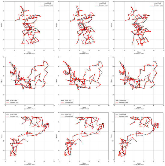
Figure 12.
Estimated paths obtained from three optimization algorithms on three random paths.
Table 2.
Error statistics for each path.
ASBOA consistently showed the lowest average error and standard deviation across all three tracks, highlighting its superior performance overall. Although the minimum errors were comparable among the three methods, there were significant differences in the maximum errors. Compared to PSO and SBOA, ASBOA demonstrated greater stability. PSO slightly outperformed SBOA in terms of both average and standard errors, though the gap was not particularly large. The results for ASBOA were unexpectedly strong, as it outperformed the other methods in both random location tracking and random path tracking.
Overall, aside from GD and SA, the other three algorithms deliver improved localization results in this mode. Upon closer comparison, ASBOA demonstrates greater stability and lower localization errors within this system, performing well in both random location and random path simulations. Although PSO’s overall localization performance is slightly inferior to ASBOA, it still surpasses SBOA, offering relatively high localization accuracy. In contrast, SBOA’s localization precision is lower but generally acceptable in most scenarios. As for GD and SA, these algorithms struggle to achieve accurate localization in this mode. Their tendency to fall into local optima, due to the problem’s complexity, leads to significant localization errors.
However, the current analysis is conducted within a simulated environment. In real-world conditions, the influence of environmental factors on RSSI and CTE signals may differ from the idealized model, and other variables, such as signal interference, must also be taken into account. Research has indicated that heavy rain can disrupt 2.4 GHz signals, causing instability. Furthermore, fluctuations in humidity and temperature can alter the environment, thereby affecting the signals. Considering these factors, it is crucial to empirically test how such extreme conditions affect Bluetooth signal integrity in real-world scenarios. This will be an area for future investigation.
6. Conclusions
This study proposes a novel outdoor positioning method based on RSSI and AOA. The method reconstructs the positioning task as an optimization problem, using optimization algorithms to minimize the root mean square error (RMSE) between the measured and estimated values, thereby ultimately determining the target’s coordinates. All simulations are conducted in an outdoor environment, using a two-ray ground reflection model as the transmission model. Overall, when evaluating the performance of different optimization algorithms for random positioning, ASBOA, PSO, and SBOA provide satisfactory positioning results, while SA and GD exhibit poor performance. Among these, the ASBOA results in the smallest positioning error, achieving an average error of 0.47 m in static point positioning and the lowest 0.65 m in dynamic tracking positioning.
Given that various scenarios utilize distinct propagation models, we believe this method can be adapted for indoor localization or other environments by substituting the propagation model. In future work, we plan to assess the practicality of this approach using real-world data. Moreover, to enhance the system’s positioning accuracy and stability, particularly under varying environmental conditions, integrating additional sensors or positioning technologies may be necessary.
Author Contributions
Conceptualization, W.B. and Y.W.; methodology, W.B. and Y.W.; software, W.B.; validation, W.B. and Y.W.; formal analysis, W.B.; investigation, W.B.; resources, Y.W.; data curation, W.B.; writing—original draft preparation, W.B.; writing—review and editing, W.B. and Y.W.; visualization, Y.W.; supervision, Y.W.; project administration, Y.W. and Y.L.; funding acquisition, Y.W. All authors have read and agreed to the published version of the manuscript.
Funding
This study was supported in part by the National Natural Science Foundation of China under grant number 32171788 and, in part, by the Qing Lan Project of Jiangsu colleges and universities.
Data Availability Statement
All data generated or presented in this study are available upon request from the corresponding author. Furthermore, the models and code used during this study cannot be shared at this time as the data also form part of an ongoing study.
Conflicts of Interest
The authors declare no conflicts of interest.
References
- Yan, G.Z.; Li, W.Y. Research on Application of Information Technology and Mathematical Modeling in Precision Agriculture. In Proceedings of the International Conference on Industrial and Information Systems, Haikou, China, 24–25 April 2009; pp. 228–231. [Google Scholar]
- Haji-Aghajany, S.; Rohm, W.; Kryza, M.; Smolak, K. Machine Learning-Based Wet Refractivity Prediction Through GNSS Troposphere Tomography for Ensemble Troposphere Conditions Forecasting. IEEE Trans. Geosci. Remote Sens. 2024, 62, 1–18. [Google Scholar] [CrossRef]
- Suo, L.; Ma, H.; Jiao, W.; Liu, X. Job-Deadline-Guarantee-Based Joint Flow Scheduling and Routing Scheme in Data Center Networks. Sensors 2024, 24, 216. [Google Scholar] [CrossRef] [PubMed]
- Thomas, C.S.; Skinner, P.W.; Fox, A.D.; Greer, C.A.; Gubler, W.D. Utilization of GIS/GPS-based information technology in commercial crop decision making in California, Washington, Oregon, Idaho, and Arizona. J. Nematol. 2002, 34, 200–206. [Google Scholar] [PubMed]
- Stone, M.L.; Benneweis, R.K.; Van Bergeijk, J. Evolution of electronics for mobile agricultural equipment. Trans. ASABE 2008, 51, 385–390. [Google Scholar] [CrossRef]
- Biswas, N.; Aslekar, A. Improving Agricultural Productivity: Use of Automation and Robotics. In Proceedings of the International Conference on Decision Aid Sciences and Applications (DASA), Chiangrai, Thailand, 23–25 March 2022; pp. 1098–1104. [Google Scholar]
- Li, C.; Jiang, L.; Ma, Q.; Teng, Y.; Bian, R.; Yu, M.; Hua, M.; Liu, X.; He, J.; Su, R.; et al. Electrically Tunable Terahertz Switch Based on Superconducting Subwavelength Hole Arrays. Appl. Opt. 2021, 60, 7530–7535. [Google Scholar] [CrossRef] [PubMed]
- Cheein, F.A.A.; Carelli, R. Agricultural Robotics Unmanned Robotic Service Units in Agricultural Tasks. IEEE Ind. Electron. Mag. 2013, 7, 48–58. [Google Scholar] [CrossRef]
- Cai, J.P.; Yao, Y.X. Application of Computer Technology in Maize Production Implementation Precision Agriculture. In Proceedings of the 4th International Conference on Intelligent System and Applied Material (GSAM), Taiyuan, China, 23–24 August 2014; pp. 1985–1988. [Google Scholar]
- Faragher, R.; Harle, R. Location Fingerprinting with Bluetooth Low Energy Beacons. IEEE J. Sel. Areas Commun. 2015, 33, 2418–2428. [Google Scholar] [CrossRef]
- Davidson, P.; Piché, R. A Survey of Selected Indoor Positioning Methods for Smartphones. IEEE Commun. Surv. Tutor. 2017, 19, 1347–1370. [Google Scholar] [CrossRef]
- Hoang, M.T.; Yuen, B.; Dong, X.D.; Lu, T.; Westendorp, R.; Reddy, K. Recurrent Neural Networks for Accurate RSSI Indoor Localization. IEEE Internet Things J. 2019, 6, 10639–10651. [Google Scholar] [CrossRef]
- Obeidat, H.; Shuaieb, W.; Obeidat, O.; Abd-Alhameed, R. A Review of Indoor Localization Techniques and Wireless Technologies. Wirel. Pers. Commun. 2021, 119, 289–327. [Google Scholar] [CrossRef]
- Zhu, X.Q.; Qiu, T.; Qu, W.Y.; Zhou, X.B.; Atiquzzaman, M.; Wu, D.O. BLS-Location: A Wireless Fingerprint Localization Algorithm Based on Broad Learning. IEEE Trans. Mob. Comput. 2023, 22, 115–128. [Google Scholar] [CrossRef]
- Ye, H.Y.; Yang, B.; Long, Z.Q.; Dai, C.H. A Method of Indoor Positioning by Signal Fitting and PDDA Algorithm Using BLE AOA Device. IEEE Sens. J. 2022, 22, 7877–7887. [Google Scholar] [CrossRef]
- Sun, Y.; Finnerty, P.; Ohta, C. BLE-Based Outdoor Localization with Two-Ray Ground-Reflection Model Using Optimization Algorithms. IEEE Access 2024, 12, 45164–45175. [Google Scholar] [CrossRef]
- Li, C.; Teng, Y.; Chen, H.; Su, R.; Sun, H.; Jiang, L. Superconducting Complementary Metamaterial-Based Switchable Device for Terahertz Wave Manipulation. Phys. Status Solidi 2023, 260, 2300203. [Google Scholar] [CrossRef]
- Qureshi, U.M.; Umair, Z.; Duan, Y.X.; Hancke, G.P. Analysis of Bluetooth Low Energy (BLE) based Indoor Localization System with Multiple Transmission Power Levels. In Proceedings of the 27th IEEE International Symposium on Industrial Electronics (ISIE), Cairns, Australia, 13–15 June 2018; pp. 1302–1307. [Google Scholar]
- Pelant, J.; Tlamsa, Z.; Benes, V.; Polak, L.; Kaller, O.; Bolecek, L.; Kufa, J.; Sebesta, J.; Kratochvil, T. BLE Device Indoor Localization Based on RSS Fingerprinting Mapped by Propagation Modes. In Proceedings of the 27th International Conference on Radioelektronika (RADIOELEKTRONIKA), Brno, Czech Republic, 19–20 April 2017; pp. 142–146. [Google Scholar]
- Vicente, D.; Tomic, S.; Beko, M.; Dinis, R.; Tuba, M.; Bacanin, N. Kalman Filter for Target Tracking Using Coupled RSS and AoA Measurements. In Proceedings of the 13th International Wireless Communications and Mobile Computing Conference (IWCMC), Valencia, Spain, 26–30 June 2017; pp. 2004–2008. [Google Scholar]
- Li, C.; Xiang, X.; Wang, P.; Teng, Y.; Chen, H.; Li, W.; Yang, S.; Chen, B.; Zhang, C.; Wu, J.; et al. Imaging-Based Terahertz Pixelated Metamaterials for Molecular Fingerprint Sensing. Opt. Express 2024, 32, 27473. [Google Scholar] [CrossRef] [PubMed]
- Zafari, F.; Gkelias, A.; Leung, K.K. A Survey of Indoor Localization Systems and Technologies. IEEE Commun. Surv. Tutor. 2019, 21, 2568–2599. [Google Scholar] [CrossRef]
- Li, Y.Y.; Qi, G.Q.; Sheng, A.D. Performance Metric on the Best Achievable Accuracy for Hybrid TOA/AOA Target Localization. IEEE Commun. Lett. 2018, 22, 1474–1477. [Google Scholar] [CrossRef]
- Chang, S. Localization based on TDoA projection for autonomous vehicles in 6G cellular networks. ICT Express 2024, 10, 34–38. [Google Scholar] [CrossRef]
- Toasa, F.A.; Tello-Oquendo, L.; Peñafiel-Ojeda, C.R.; Cuzco, G. Experimental Demonstration for Indoor Localization Based on AoA of Bluetooth 5.1 Using Software Defined Radio. In Proceedings of the IEEE 18th Annual Consumer Communications and Networking Conference (CCNC), Las Vegas, NV, USA, 9–12 January 2021. [Google Scholar]
- Fu, Y.; Liu, D.; Chen, J.; He, L. Secretary bird optimization algorithm: A new metaheuristic for solving global optimization problems. Artif. Intell. Rev. 2024, 57, 123. [Google Scholar] [CrossRef]
- Samokhin, A.B.; Samokhina, A.S.; Sklyar, A.Y.; Shestopalov, Y.V. Iterative Gradient Descent Methods for Solving Linear Equations. Comput. Math. Math. Phys. 2019, 59, 1267–1274. [Google Scholar] [CrossRef]
- Yang, X.J.; Jiao, Q.J.; Liu, X.K. Center Particle Swarm Optimization Algorithm. In Proceedings of the IEEE 3rd Information Technology, Networking, Electronic and Automation Control Conference (ITNEC), Chengdu, China, 15–17 March 2019; pp. 2084–2087. [Google Scholar]
Disclaimer/Publisher’s Note: The statements, opinions and data contained in all publications are solely those of the individual author(s) and contributor(s) and not of MDPI and/or the editor(s). MDPI and/or the editor(s) disclaim responsibility for any injury to people or property resulting from any ideas, methods, instructions or products referred to in the content. |
© 2024 by the authors. Licensee MDPI, Basel, Switzerland. This article is an open access article distributed under the terms and conditions of the Creative Commons Attribution (CC BY) license (https://creativecommons.org/licenses/by/4.0/).