Bi-PredRNN: An Enhanced PredRNN++ with a Bidirectional Network for Spatiotemporal Sequence Prediction

Abstract

In recent years, significant advancements have been made in spatiotemporal sequence prediction, with PredRNN++ emerging as a powerful model due to its superior ability to capture complex temporal dependencies. However, the current unidirectional nature of PredRNN++ limits its ability to fully exploit the temporal information inherent in many real-world sequences. In this research, we propose an enhancement to the PredRNN++ model by incorporating a bidirectional network, enabling the model to consider both past and future contexts during prediction. This bidirectional extension enhances the model’s ability to predict sequences accurately and reliably, especially for data with intricate temporal patterns. Our experimental results demonstrate that the Bidirectional PredRNN++ outperforms the original model across several benchmark datasets, highlighting its potential for a wide range of applications in spatiotemporal data analysis.

1. Introduction

Spatiotemporal data integrate spatial information with temporal progression and form multidimensional datasets. Previous studies have contributed to a foundational understanding of spatiotemporal data, including their statistical characteristics [1,2], visualization techniques [3], and predictive frameworks [4], which are essential for defining the scope and challenges addressed in this study. Understanding spatiotemporal data requires effectively processing both spatial and temporal components, which are inherently more intricate and diverse than traditional data while incorporating both spatial and temporal aspects. Predictive analytics [5] plays a crucial role in understanding complex spatiotemporal data patterns. By analyzing previous and current data patterns, predictive analytics enables the forecasting of future events and helps identify emerging trends and behaviors [6,7].

These predictive capabilities have become essential in modern AI and electronic applications. For instance, autonomous driving systems require the precise prediction of surrounding object trajectories by analyzing continuous sequences of spatial positions and temporal patterns [8,9]. In smart manufacturing, the analysis of time-series sensor data, combined with spatial equipment states, enables the early detection of potential failures [10]. Weather forecasting systems integrate multiple spatiotemporal variables, such as temperature, pressure, and wind patterns, to predict severe weather events over time [11,12,13]. These applications highlight the critical importance of developing technologies that can predict future frames based on given sequences of spatiotemporal data.

Traditional approaches to spatiotemporal prediction problems have evolved through several key developments in deep learning architectures. Recurrent Neural Networks (RNNs) [14] and their variant Long Short-Term Memory (LSTM) networks [15] laid the foundation for sequential data processing through their ability to model temporal dependencies. Building on these concepts, Spatiotemporal LSTM (ST-LSTM) [16] introduced a dual-memory structure that integrates spatial and temporal dependencies, serving as a precursor to the enhanced dual-memory mechanism adopted in Causal LSTM. However, these architectures still face significant challenges in modeling complex spatiotemporal dependencies. While they successfully preserve high-level features, they often struggle to maintain fine-grained spatial details over long sequences [4].

The introduction of PredRNN [17] marked a significant advancement in addressing these limitations. This architecture implements a dual-memory mechanism: local memory cells for preserving detailed spatial information and a global memory flow for capturing high-level temporal dynamics. PredRNN++ [18] further enhanced this approach by introducing gradient highway units to facilitate better gradient flow during training. PredRNN-v2 [19] added memory decoupling and reverse scheduled sampling, improving the model’s ability to learn from longer temporal contexts.

Unidirectional models such as PredRNN++ focus solely on processing past temporal information to predict future states. While effective in capturing historical dependencies, they are inherently limited in their ability to utilize future temporal context, which can be critical in many spatiotemporal prediction tasks. For instance, in chaotic or highly dynamic systems, the absence of future context often results in inaccurate predictions or an over-reliance on prior states. In contrast, bidirectional processing [20,21,22] enables the integration of both past and future temporal dependencies, offering a more holistic view of the temporal sequence. This approach allows the model to dynamically reconcile inconsistencies between past observations and potential future outcomes, thereby improving prediction robustness and accuracy. For example, in applications such as climate modeling, future temperature trends may provide critical context for interpreting past patterns, leading to more reliable forecasts. The proposed Bi-PredRNN addresses these limitations by introducing a bidirectional memory mechanism, which processes information in both the forward and backward directions. This dual-path memory flow not only captures comprehensive temporal dependencies but also mitigates the vanishing gradient problem through enhanced gradient propagation pathways.

Building upon these insights, we propose Bi-PredRNN, an enhanced architecture that extends the PredRNN framework with bidirectional processing capabilities. Our model makes two key contributions:

• A bidirectional memory mechanism that processes temporal information in both the forward and backward directions, enabling more comprehensive temporal context modeling;
• A mechanism that adapts the temporal window size based on the input’s motion complexity.

We evaluated our model on three diverse datasets: Moving MNIST (digit sequences), KTH Action (human motion), and climate data, considering both short and long temporal horizons. The temporal horizon defines the number of future time steps predicted by the model, demonstrating its flexibility in handling varying temporal scales. We demonstrate that Bi-PredRNN achieves superior prediction accuracy compared to existing approaches. The rest of this paper details our methodology, experimental validation, and analysis of results. Section 2 reviews related work in spatiotemporal sequence prediction, Section 3 describes our proposed architecture, Section 4 and Section 5 presents the experimental setup and results, and Section 6 concludes with discussions and future directions.

2. Related Works

2.1. Overview of Spatiotemporal Sequence Prediction

Spatiotemporal sequence prediction involves predicting future data points by analyzing both spatial and temporal dependencies in a sequence of data. This type of prediction is crucial for applications such as video processing, weather forecasting, and traffic flow prediction. Challenges arise from the need to capture two aspects: spatial correlations that represent relationships between different locations and temporal dynamics that describe the evolution of these relationships. The spatial aspect of prediction involves understanding relationships between different locations or features in a given space. Yu et al. [23] formalized this as a graph structure, where nodes represent spatial locations and edges capture their interactions, in their seminal work on traffic forecasting. This graph-based framework has become fundamental in modern approaches to spatiotemporal modeling. For grid-structured data, Shi et al. [4] introduced the ConvLSTM architecture, which effectively captures spatiotemporal correlations in regular grids, establishing a foundation for applications like precipitation forecasting. Temporal dependencies capture how patterns evolve over time, often exhibiting both short-term and long-term characteristics, requiring models to capture multiple temporal scales simultaneously.

2.2. Spatiotemporal Convolutional Neural Networks

Spatiotemporal Convolutional Neural Networks (CNNs) extend traditional 2D CNNs to capture temporal dynamics in video data. In ConvLSTM architectures [4], LSTM cells are fundamentally redesigned to accommodate convolutional operations, effectively modeling spatial and temporal dependencies. This foundation directly informs the dual-memory mechanisms in our Bi-PredRNN model.

In [4], the authors combined graph convolutional layers composed of spatiotemporal convolutional blocks with a convolutional sequence learning layer, utilizing the convolutional structure along the time axis to fully leverage spatial information. Recent advances have also focused on memory-efficient implementations and real-time processing capabilities, introducing innovations in sparse convolution techniques [24] and adaptive temporal sampling strategies [25].

2.3. Spatiotemporal Long Short-Term Memory

LSTM networks have advanced from basic sequence modeling to tackling spatiotemporal prediction challenges [15]. By integrating spatial and temporal features, architectures like ST-LSTM [16] process these streams simultaneously, capturing spatiotemporal dependencies effectively. Building on ST-LSTM and ConvLSTM, the Memory In Memory (MIM) network [26] introduced a sophisticated mechanism to model higher-order non-stationary transitions, excelling in complex, multi-frequency prediction tasks.

Figure 1 highlights the differences in how these architectures handle spatial and temporal dependencies, with CausalLSTM focusing on improving long-term memory.

2.4. Multi-Modal Prediction and Attention Models

Recent advancements in spatiotemporal prediction have introduced attention mechanisms and transformer-based architectures that enable the direct modeling of long-range dependencies. These approaches are increasingly popular for handling the growing complexity of real-world spatiotemporal data. While Bi-PredRNN focuses on enhancing traditional RNN-based frameworks through bidirectional processing and adaptive memory mechanisms, the broader field continues to explore alternative paradigms, such as multi-modal integration and graph-based frameworks. These developments complement the goals of Bi-PredRNN by addressing challenges in different dimensions, highlighting the diverse approaches within the domain of spatiotemporal prediction.

Recent advancements in spatiotemporal prediction have seen promising results in incorporating multi-modal data and handling complex interaction patterns. Junan Chen et al. [27] proposed a spatiotemporal graph neural network that explicitly models vehicle interactions for trajectory prediction. Their approach combines attention mechanisms with graph neural networks to capture both spatial relationships and temporal dependencies between vehicles in complex traffic scenarios. The integration of self-supervised learning techniques has also shown promise in improving spatiotemporal forecasting. Weyn et al. [28] introduced a novel multi-modality framework that leverages self-supervised learning to capture correlations across different data modalities. Their approach addresses the challenge of learning from multiple data sources while maintaining computational efficiency, particularly valuable for applications involving diverse sensor inputs. Furthermore, environmental monitoring applications have driven innovations in handling missing data in spatiotemporal sequences. Nejad et al. [29] developed SERT, a transformer-based architecture specifically designed for environmental sensor data with missing values. Their model combines spatial and temporal attention mechanisms with specialized embedding techniques to handle irregular sampling and missing observations, demonstrating robust performance in real-world environmental monitoring scenarios.

2.5. Limitations of Current Approaches

Recent advances in spatiotemporal prediction models have demonstrated significant progress in capturing complex temporal dependencies and spatial relationships. However, several fundamental limitations persist in current approaches and reduce their effectiveness in real-world applications. This section analyzes these limitations and presents our research position addressing these challenges.

A primary challenge in RNN-based architectures is the persistent issue of vanishing gradients during backpropagation through time (BPTT) [30]. While various techniques such as gradient clipping and careful initialization have been proposed [31], these solutions provide only partial remedies and often fail in scenarios requiring long-term dependency modeling [32]. This limitation is especially evident in long-term predictions like weather forecasting and traffic analysis.

The integration of spatial and temporal features presents another significant challenge. Traditional Fully Connected LSTM architectures, by treating spatial information as flat vectors, inherently lose crucial spatial relationships that are essential for accurate prediction [4]. Although ConvLSTM architectures have attempted to address this by introducing spatial operations, they still struggle with maintaining long-range spatial dependencies effectively [33]. The fundamental trade-off between preserving spatial features and maintaining temporal memory remains suboptimal, particularly in scenarios involving complex spatial transformations [18].

Data efficiency and scalability concerns significantly impact the practical deployment of current models. Transformer-based approaches, despite their powerful representation capabilities, exhibit considerable data hunger due to their limited inductive biases [34]. The computational cost increases quadratically with the sequence length, which imposes practical challenges on their application to long sequences [35]. Furthermore, the extensive pre-training requirements make these models particularly resource-intensive for specialized domains. This makes them inaccessible to researchers with limited computational resources [36].

Model adaptability represents another critical limitation. For example, current approaches like 3D CNN with DropPath, a regularization technique, often require complete retraining for new datasets, limiting their practical utility in dynamic environments [37]. This lack of transfer learning capabilities not only increases computational overhead but also limits the models’ practical utility in real-world scenarios where data distributions may shift over time [38]. The challenge of domain adaptation becomes particularly acute in specialized architectures, where the model’s performance can degrade significantly when applied to slightly different domains.

3. Method

In this section, we present a comprehensive description of our proposed Bidirectional Predictive Recurrent Neural Network (Bi-PredRNN). Our methodology introduces two principal contributions to the field of spatiotemporal prediction. First, we propose a novel bidirectional memory network architecture that systematically integrates both antecedent and subsequent temporal information into the feature representation process. This approach enables more robust modeling of long-term dependencies through detailed temporal context utilization. Second, we demonstrate the model’s versatility across diverse data representations, successfully applying it to both regular grid-structured data (e.g., 2D dynamics) and complex irregular spatiotemporal patterns (e.g., climate datasets). This cross-domain applicability validates the generalization of our approach across varying data representations and temporal scales.

3.1. Bidirectional Memory

We enhance temporal context modeling by incorporating bidirectional processing into our memory architecture. The introduction of bidirectional processing represents a significant paradigm shift in spatiotemporal prediction for several key reasons [20,21,22]. As highlighted in Section 2.5, traditional unidirectional models suffer from information bottlenecks and limited temporal context due to their reliance on past information. The dual-memory approach in Bi-PredRNN addresses these issues by creating a robust feature representation mechanism through bidirectional memory integration. As illustrated in Figure 2, our bidirectional approach enables more comprehensive context utilization through dual paths of information flow, significantly mitigating the vanishing gradient problem through multiple gradient propagation routes.

Bi-PredRNN uses two memory streams to capture richer temporal patterns by capturing both the forward and backward temporal dependencies simultaneously. The forward path maintains the causal relationships essential for prediction, while the backward path incorporates future context that enables more accurate long-term forecasting [17,18]. This comprehensive approach to temporal modeling allows the network to leverage a more complete set of spatiotemporal relationships. This design enables the model to accurately capture complex spatiotemporal relationships while maintaining computational efficiency. This is achieved through the bidirectional memory architecture, which processes temporal dependencies and spatial information independently before integrating them into a unified representation. By preserving critical spatial details during this integration, the model avoids information loss, which often occurs in other approaches. Furthermore, the bidirectional information flow minimizes redundant computations, allowing the model to sustain high performance even for long sequences.

Our model implements several key contributions to enhance its effectiveness. First, the dual-memory integration mechanism maintains spatial coherence through specialized memory cells while enabling efficient information flow between the forward and backward paths. Second, the enhanced feature capture mechanism preserves spatial relationships through structured memory organization, ensuring that critical spatial information is not lost during temporal processing. Finally, our adaptive processing framework dynamically adjusts feature importance through learned attention mechanisms, balancing computational efficiency with model expressiveness.

Bi-PredRNN introduces a bidirectional memory mechanism that processes sequences in both the forward and backward directions. The forward path captures causal dependencies from past observations, while the backward path processes the same input sequence in reverse order to learn temporal dependencies from the opposite direction. By combining these two streams, the model creates a unified temporal representation, effectively capturing bidirectional dynamics during training. During inference, only the forward path is utilized to generate future predictions, as future observations are unavailable.

This bidirectional processing not only enriches temporal modeling but also mitigates the vanishing gradient problem. Gradients propagate through both forward and backward paths, ensuring stability during the learning process and improving the model’s capacity to handle long sequences.

To enhance its effectiveness, Bi-PredRNN integrates spatial coherence with temporal dependencies. It achieves this through memory cells that preserve spatial information while enabling efficient flow between forward and backward streams. These design choices allow the model to accurately capture complex spatiotemporal relationships while maintaining computational efficiency.

3.2. Theoretical Framework of Bidirectional Memory Flow

Let $X=\{x_1,x_2,\dots ,x_T\}$ be a spatiotemporal sequence, where $x_t\in {\mathbb{R}}^{H\times W\times C}$ represents a spatial state at time $t\in \{1,\dots ,T\}$ with height H, width W, and channels C. The bidirectional memory flow operates by maintaining two complementary hidden states: a forward hidden state $\overrightarrow{h_t}$ that processes the sequence from $t=1$ to T, and a backward hidden state $\overleftarrow{h_t}$ that processes from $t=T$ to 1. As illustrated in Figure 2, these bidirectional paths are implemented through cascaded memory cells with convolution operations and layer normalization.

The core principle of this architecture is to integrate both causal and predictive patterns through bidirectional processing. At each time step t, the complete representation $h_t$ is derived from these bidirectional states:

$$\begin{array}{cc}\hfill \overrightarrow{h_t}& =\psi (\overrightarrow{h_{t-1}},x_t,{\theta }_{\overrightarrow{f}})\hfill \\ \hfill \overleftarrow{h_t}& =\psi (\overleftarrow{h_{t+1}},x_t,{\theta }_{\overleftarrow{b}})\hfill \\ \hfill h_t& =\varphi (\overrightarrow{h_t},\overleftarrow{h_t}),\hfill \end{array}$$

where $\psi$ denotes the memory update function, ${\theta }_{\overrightarrow{f}}$ and ${\theta }_{\overleftarrow{b}}$ are the learnable parameters for forward and backward processes, respectively, and $\varphi$ represents the fusion function that integrates the bidirectional information. The memory update function incorporates both spatial and temporal dependencies through a CausalLSTM [18] architecture:

$$\begin{array}{cc}\hfill i_t& =\sigma (W_{xi}{x}_t+W_{hi}\overrightarrow{h_{t-1}}+b_i)\hfill \\ \hfill f_t& =\sigma (W_{xf}{x}_t+W_{hf}\overrightarrow{h_{t-1}}+b_f)\hfill \\ \hfill c_t& =f_t\odot c_{t-1}+i_t\odot tanh(W_{xc}{x}_t+W_{hc}\overrightarrow{h_{t-1}}+b_c)\hfill \\ \hfill o_t& =\sigma (W_{xo}{x}_t+W_{ho}\overrightarrow{h_{t-1}}+b_o)\hfill \\ \hfill \overrightarrow{h_t}& =o_t\odot tanh\left(c_t\right),\hfill \end{array}$$

where $\sigma$ represents the sigmoid activation function, and ⊙ indicates element-wise multiplication between matrices.

3.3. Training Strategy and Loss Functions

The training of Bi-PredRNN employs a carefully designed loss function that addresses multiple aspects of spatiotemporal prediction quality. The total loss is composed of three main components:

$${\mathcal{L}}_{total}={\lambda }_1{\mathcal{L}}_{reconstruction}+{\lambda }_2{\mathcal{L}}_{temporal}+{\lambda }_3{\mathcal{L}}_{consistency}$$

(1)

The first term, reconstruction loss, ensures accurate frame-level predictions by minimizing the mean squared error between predicted and ground-truth frames:

$${\mathcal{L}}_{reconstruction}={\displaystyle \frac{1}{T}}\sum _{t=1}^T{\parallel x_t-{\widehat{x}}_t\parallel }_2^2,$$

(2)

where $x_t$ and ${\widehat{x}}_t$ denote the ground-truth and predicted frames at time step t, respectively. This loss ensures smooth temporal transitions by matching the dynamics between consecutive frames, reducing artifacts such as jittering or abrupt changes. The mean is calculated over all T − 1 frame transitions.

The second term introduces temporal coherence by penalizing inconsistencies in frame-to-frame transitions:

$${\mathcal{L}}_{temporal}={\displaystyle \frac{1}{T-1}}\sum _{t=1}^{T-1}{\parallel \mathrm{\Delta }{x}_t-\mathrm{\Delta }{\widehat{x}}_t\parallel }_2^2,$$

(3)

where $\mathrm{\Delta }{x}_t=x_{t+1}-x_t$ represents frame-to-frame differences. This loss ensures smooth temporal transitions by matching the dynamics between consecutive frames in both predicted and ground-truth sequences, reducing temporal artifacts such as jittering or sudden changes.

The third term, bidirectional consistency loss, enforces agreement between forward and backward predictions:

$${\mathcal{L}}_{consistency}={\displaystyle \frac{1}{T}}\sum _{t=1}^T{\parallel {\overrightarrow{h}}_t-{\overleftarrow{h}}_t\parallel }_2^2,$$

(4)

where ${\overrightarrow{h}}_t$ and ${\overleftarrow{h}}_t$ represent the hidden states from forward and backward passes, respectively. This loss term encourages the model to learn consistent representations regardless of the sequence direction, leading to more robust predictions.

The coefficients ${\lambda }_1$, ${\lambda }_2$, and ${\lambda }_3$ are set to 1.0, 0.5, and 0.2, respectively, based on empirical validation. These weights balance the contribution of each loss component, with higher weight on reconstruction accuracy while maintaining temporal coherence and bidirectional consistency. This allocation reflects the relative importance of the loss components: Reconstruction loss ($L_{\mathrm{reconstruction}}$) is critical for pixel-level accuracy and thus given the highest weight. Temporal coherence loss ($L_{\mathrm{temporal}}$) balances frame-to-frame dynamics, warranting a moderate weight. Finally, bidirectional consistency loss ($L_{\mathrm{consistency}}$) supports stable learning but serves as a secondary objective, justifying a lower weight. This balance ensures the model prioritizes reconstruction accuracy while maintaining temporal and directional consistency.

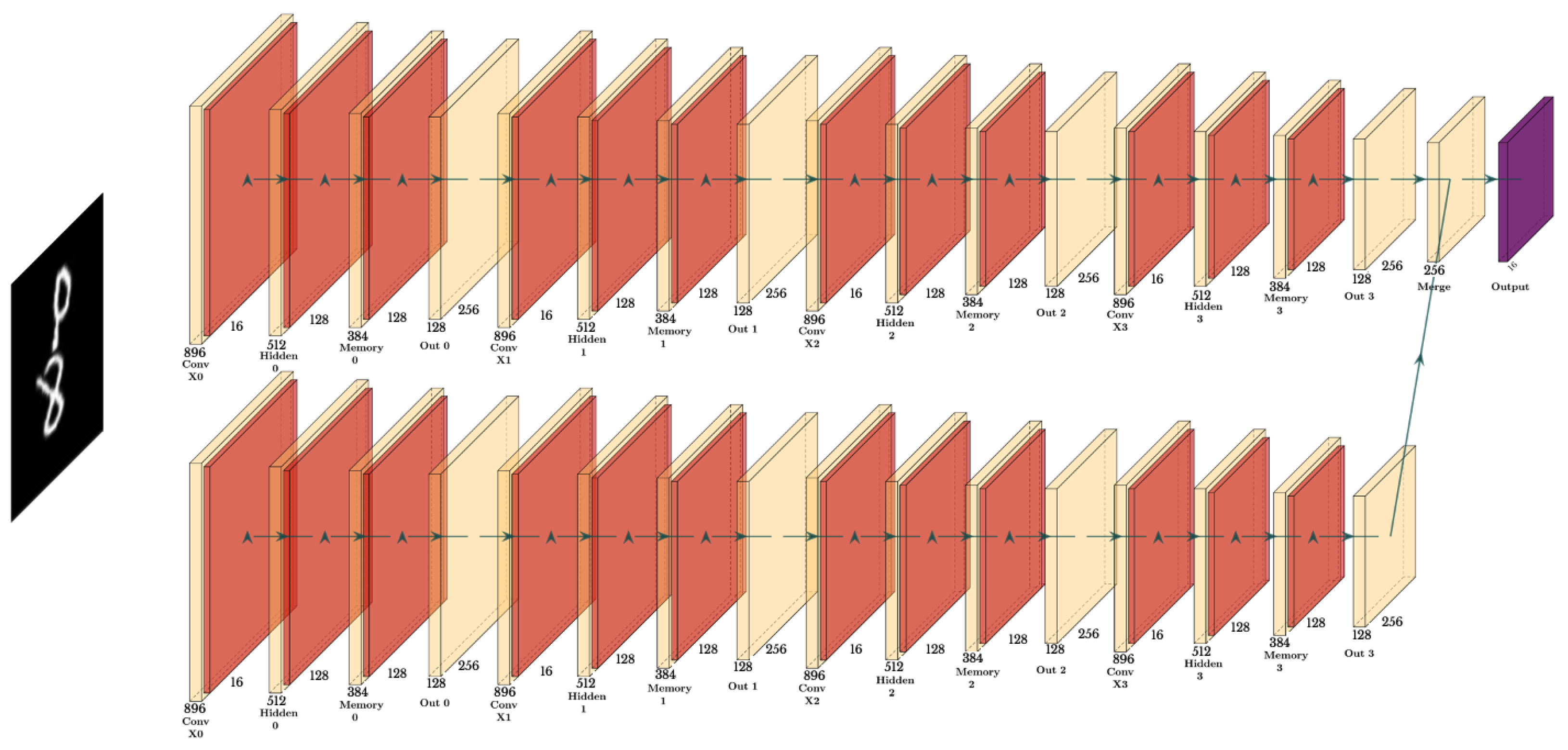
3.4. Multi-Layer Implementation

The theoretical framework is implemented through a K-layer architecture, where each layer $k\in \{1,\dots ,K\}$ maintains its hidden state $h_t^k$ and cell state $c_t^k$. Although deeper architectures generally enable the capture of more sophisticated features, we adopt the widely used 4-layer configuration (K = 4) that has been empirically validated across various spatiotemporal prediction tasks. As illustrated in Figure 3, the network processes information in both the forward and backward directions. This utilizes a cascaded memory flow mechanism to handle time steps effectively.

The network first processes information in the forward direction. For time step t from 1 to T,

$$\begin{array}{cc}\hfill \mathrm{Layer}\mathrm{k}=1:& \overrightarrow{h_t^1},\overrightarrow{c_t^1},\overrightarrow{M_t^1}=\mathrm{CausalLSTM}(x_t,\overrightarrow{h_{t-1}^1},\overrightarrow{c_{t-1}^1},\overrightarrow{M_{t-1}^K})\hfill \\ \hfill \mathrm{Layer}\mathrm{k}>1:& \overrightarrow{h_t^k},\overrightarrow{c_t^k},\overrightarrow{M_t^k}=\mathrm{CausalLSTM}(\overrightarrow{h_t^{k-1}},\overrightarrow{h_{t-1}^k},\overrightarrow{c_{t-1}^k},\overrightarrow{M_t^{k-1}})\hfill \end{array}$$

Following the forward pass, the network processes information in the backward direction. For time step t from T to 1,

$$\begin{array}{cc}\hfill \mathrm{Layer}\mathrm{k}=1:& \overleftarrow{h_t^1},\overleftarrow{c_t^1},\overleftarrow{M_t^1}=\mathrm{CausalLSTM}(x_t,\overleftarrow{h_{t+1}^1},\overleftarrow{c_{t+1}^1},\overleftarrow{M_{t+1}^K})\hfill \\ \hfill \mathrm{Layer}\mathrm{k}>1:& \overleftarrow{h_t^k},\overleftarrow{c_t^k},\overleftarrow{M_t^k}=\mathrm{CausalLSTM}(\overleftarrow{h_t^{k-1}},\overleftarrow{h_{t+1}^k},\overleftarrow{c_{t+1}^k},\overleftarrow{M_t^{k-1}})\hfill \end{array}$$

The hidden states from forward and backward passes are first concatenated:

$$\begin{array}{cc}\hfill h_t^{combined}& =[h_t^K;\overleftarrow{h_t^K}]\hfill \end{array}$$

The final prediction for the next time step is then generated through a dimensionality reduction layer:

$$\begin{array}{cc}\hfill x_{t+1}& =\mathrm{Conv}2\mathrm{D}\left(h_t^{combined}\right),\hfill \end{array}$$

where Conv2D is a 1 × 1 convolutional layer that reduces the channel dimension to match the input dimension. This multi-layer structure enables sophisticated spatiotemporal pattern modeling through hierarchical feature extraction and bidirectional information flow. Note that in both passes, the spatial memory from the highest layer ($\overrightarrow{M_t^4}$ and $\overleftarrow{M_t^4}$) flows to the lowest layer of the next time step ($\overrightarrow{M_{t-1}^4}\to \overrightarrow{M_t^1}$ for forward pass, $\overleftarrow{M_{t+1}^4}\to \overleftarrow{M_t^1}$ for backward pass). This cascade memory flow allows the model to maintain long-term spatial dependencies across time steps while processing information bidirectionally.

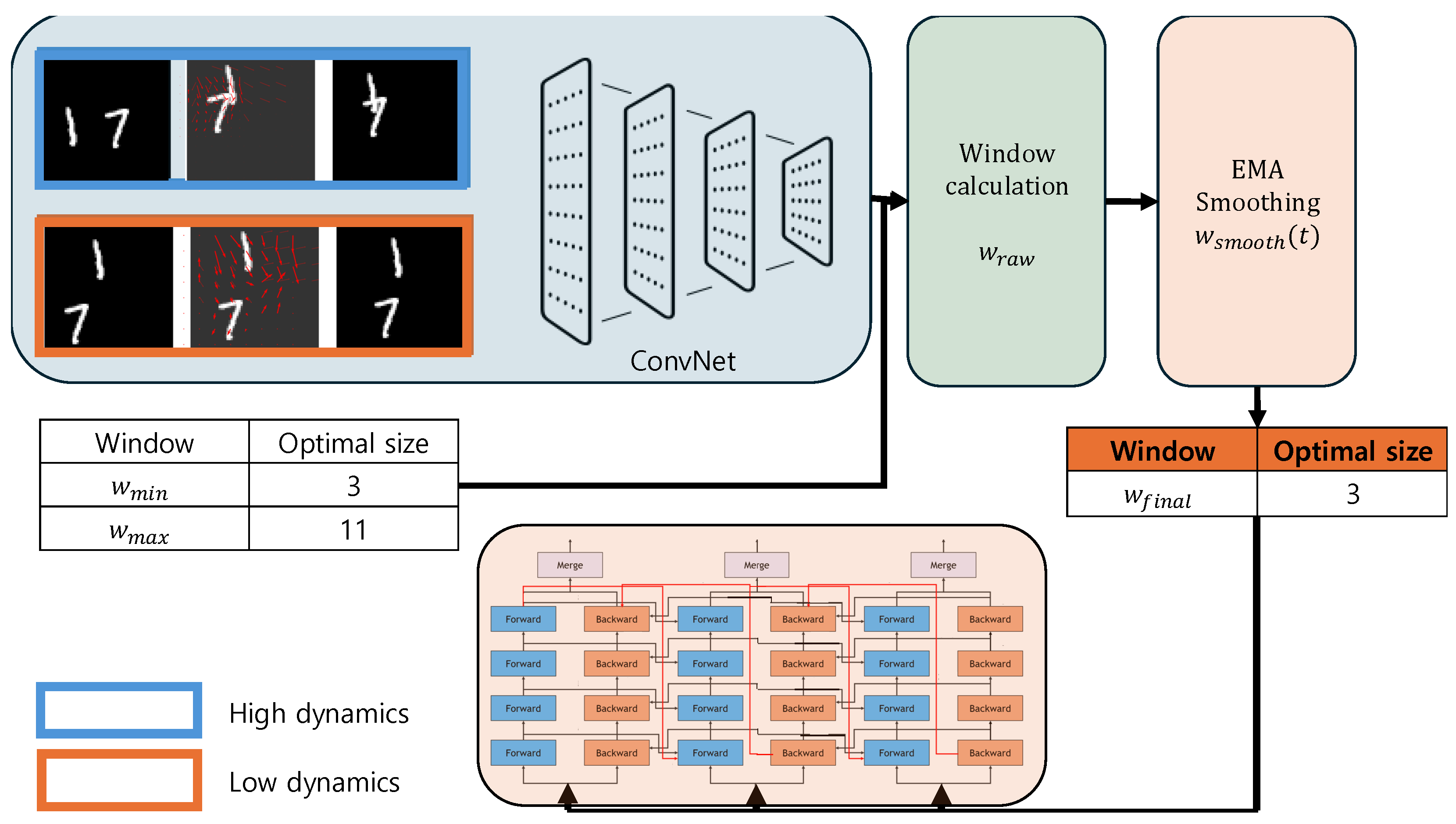
3.5. Dynamic Window Size Mechanism

We propose a dynamic window size mechanism that determines how much historical data the model should observe based on motion patterns between frames. Unlike conventional approaches that use fixed-length sequences, our method employs a CNN-based optical flow analysis to adaptively adjust the temporal window size. This means that when significant motion is detected, the model can automatically increase its observation window to capture more historical context, and conversely, the model can reduce it during periods of minimal motion to maintain computational efficiency.

The window size is governed by three parameters: minimum window size ($w_{min}=3$), maximum window size ($w_{max}=11$), and EMA smoothing coefficient ($\alpha =0.8$). The optical flow CNN analyzes frame-to-frame motion and outputs a score that determines where within this range the window size should be set. The EMA coefficient helps prevent abrupt changes in window size, ensuring smooth transitions between different temporal contexts.

3.5.1. Optical-Flow-Based Motion Estimation

The motion estimation is performed using a lightweight convolutional neural network that consists of three layers:

$$\begin{array}{}\mathrm{(5)}& \hfill f_1& =\mathrm{ReLU}\left(\mathrm{Conv}(X_{t,t+1};7\times 7,2\to 64)\right)\hfill \mathrm{(6)}& \hfill f_2& =\mathrm{ReLU}\left(\mathrm{Conv}(f_1;5\times 5,64\to 32)\right)\hfill \mathrm{(7)}& \hfill f_{\mathrm{flow}}& =\mathrm{Conv}(f_2;3\times 3,32\to 2),\hfill \end{array}$$

where $X_{t,t+1}\in {\mathbb{R}}^{H\times W\times 2}$ represents the concatenated input of two consecutive frames, and $\mathrm{Conv}(x;k,c_{in}\to c_{out})$ denotes a convolutional operation with kernel size k and channel dimensions $c_{in}\to c_{out}$. The network progressively processes the spatial information while maintaining the ability to capture motion patterns at different scales through its hierarchical structure. The motion magnitude $s_{\mathrm{motion}}$ is computed as the average magnitude of optical flow vectors across all spatial locations:

$$s_{\mathrm{motion}}={\displaystyle \frac{1}{H\times W}}\sum _{i=1}^H\sum _{j=1}^W\sqrt{{\left(f_{\mathrm{flow}}^x(i,j)\right)}^2+{\left(f_{\mathrm{flow}}^y(i,j)\right)}^2},$$

(8)

where $f_{\mathrm{flow}}^x(i,j)$ and $f_{\mathrm{flow}}^y(i,j)$ represent the horizontal and vertical components of the optical flow at spatial position $(i,j)$, respectively, and H and W are the height and width of the feature map.

3.5.2. Adaptive Window Size Selection and Adaptation

The window size is determined through a three-step process.

The Base Window Size is

$$w_{\mathrm{raw}}=w_{\min }+(w_{\max }-w_{\min })·\sigma \left(s_{\mathrm{motion}}\right),$$

(9)

where $\sigma$ is the sigmoid function that maps the motion magnitude to a value between 0 and 1, enabling smooth and nonlinear scaling. This ensures that small variations in motion result in gradual changes in $w_{\mathrm{raw}}$ while preventing extreme motion magnitudes from causing abrupt or disproportionate adjustments to the window size. Temporal Smoothing using Exponential Moving Average (EMA) is

$$w_{\mathrm{smooth}}\left(t\right)=\alpha w_{\mathrm{smooth}}(t-1)+(1-\alpha )w_{\mathrm{raw}}\left(t\right),$$

(10)

where $w_{\mathrm{smooth}}\left(t\right)$ and $w_{\mathrm{smooth}}(t-1)$ represent the smoothed window sizes at the current and previous time steps, respectively. Window Size Parity Adjustment is

$$w_{\mathrm{final}}=\left\{\begin{array}{cc}{w}_{\mathrm{smooth}}\hfill & \mathrm{if}{w}_{\mathrm{smooth}}\mathrm{is}\mathrm{odd}\hfill \\ w_{\mathrm{smooth}}+1\hfill & \mathrm{if}{w}_{\mathrm{smooth}}\mathrm{is}\mathrm{even}\hfill \end{array}\right.$$

(11)

The final window size determines the temporal context for both forward and backward passes:

$$\begin{array}{cc}\hfill t_{\mathrm{start}}& =max(0,t-\lfloor w_{\mathrm{final}}/2\rfloor )\hfill \\ \hfill t_{\mathrm{end}}& =min(T-1,t+\lfloor w_{\mathrm{final}}/2\rfloor ),\hfill \end{array}$$

(12)

where T is the total number of frames in the sequence.

Figure 4 illustrates how the dynamic window size mechanism operates in a low-dynamics scenario using the Moving MNIST dataset. The first and third images represent the initial and final positions of the digits, respectively, highlighting scenarios with significant motion (blue) and minimal motion (orange). In the orange box, the minimal change between the two positions emphasizes the low-dynamics scenario.

The second image visualizes the optical flow, where arrows represent the direction and magnitude of motion between frames. In the low-dynamics scenario (orange box), the optical flow visualization shows short and less distinct arrows, indicating minimal motion between frames. This motion pattern is analyzed by the dynamic window size mechanism, which determines the optimal window size ($w_{\mathrm{final}}=3$) based on the motion magnitude ($s_{\mathrm{motion}}$).

In the low-dynamics scenario, the mechanism assigns a small window size to maintain computational efficiency while focusing on recent frames for learning temporal dependencies. The forward pass processes the most recent frames (e.g., $t-2$ to t), and the backward pass processes the same frames in reverse order (e.g., t to $t-2$), enabling the model to effectively capture temporal relationships.

4. Experiments

We evaluated the performance of our proposed method using the following datasets: Moving MNIST, the KTH Action dataset, the ToSNA (North Atlantic) SST dataset, and the Global Climate dataset. The first two datasets are benchmarks that are widely used for sequence prediction tasks, while the latter two provide real-world climate data to validate our model’s applicability to environmental forecasting problems. All models were implemented using the PyTorch 1.9.0 framework [39] and trained until convergence using the Adam optimizer. We employed an L2 loss (mean squared error, MSE) function for all experiments and tuned the hyperparameters with the learning rate initialized at ${10}^{-3}$. Each dataset’s unique characteristics and challenges were considered when tailoring the hyperparameters. Key parameters included the number of hidden layers, latent dimension size, filter size, patch size, and the use of regularization techniques such as layer normalization. For the climate dataset, layer normalization ($laye{r}_{n}orm$ = 1) and a decoupling loss term ($decoupl{e}_{b}eta$ = 0.1) were introduced to handle its larger spatial resolution and complex temporal dependencies.

The ToSNA dataset required an additional preprocessing step to address issues encountered during patch size calculations. Specifically, zero-padding was applied to the edges of longitude and latitude (x- and y-axes) in each frame. This adjustment ensured compatibility with the patch size settings during the generation of the real input flag tensor, which splits the spatial dimensions into smaller patches for processing. By padding the edge areas of the spatial dimensions, the framework effectively handled the discrepancies in resolution without compromising data integrity.

The datasets employed in this study necessitate differing data partitioning strategies due to their inherent characteristics and purposes. For synthetic datasets like Moving MNIST, predefined splits are often used to maintain consistency with existing benchmarks. For real-world datasets such as KTH and the climate datasets, however, the splitting strategies are tailored to their specific properties and evaluation objectives. The KTH dataset uses a person-based splitting strategy to assess generalization across unseen individuals, while the climate datasets follow a temporally coherent splitting strategy to capture long-term spatiotemporal dependencies in environmental data. These approaches ensure that the evaluation is aligned with the unique challenges posed by each dataset.

4.1. Moving MNIST Dataset

For the Moving MNIST dataset [40], we evaluated our model’s predictive performance by generating 10 future frames given 10 input frames. The dataset consists of sequences where digits move and bounce within a 64 × 64 pixel frame. The input data are structured with a clips array of shape (2 × 10,000 × 2), where 2 represents the number of moving digits, 10,000 represents the number of data samples, and 2 represents the $x,y$-coordinates of each digit; a dims array of shape $(1,3)$, where 1 is the batch size, and 3 represents spatial dimensions; and an input_raw_data array of shape (200,000 × 1 × 64 × 64), where 200,000 is the total number of frames, 1 represents the channel number (grayscale), and $64\times 64$ represents the height and width of the image in pixels. The raw input data have a mean pixel value of 0.047 and a standard deviation of 0.194, indicating a sparse presence of digits in the frames. We split the dataset into 10,000 training sequences and 3000 validation sequences, with digits in the validation set drawn from different portions of the MNIST dataset than those used in training. The Moving MNIST dataset is provided with predefined training and validation splits to ensure consistency in benchmarking. We adhered to these splits to maintain comparability with prior works.

4.2. KTH Dataset

For the KTH dataset [41], we evaluated our model’s predictive performance by generating 10 future frames given 10 input frames. The dataset consists of sequences where human subjects perform six types of actions (walking, jogging, running, boxing, hand waving, and hand clapping) in four different scenarios (outdoors, outdoors with scale variation, outdoors with different clothes, and indoors). Each sequence was recorded at 25fps and downsampled to $160\times 120$ pixel frames. The input data are structured with an input_raw_data array of shape (N × 1 × 120 × 160), where N represents the total number of frames across all sequences, 1 represents the grayscale channel, and $120\times 160$ represents the height and width of the image in pixels. The raw input data have been preprocessed to normalize pixel values between 0 and 1, with background pixels typically having values close to 0 and the foreground (human subjects) showing higher intensity values.

To evaluate the model’s ability to generalize across unseen subjects, we adopted a person-based splitting strategy. This strategy ensures that sequences from the same individuals are excluded from both training and test sets. Specifically, 16 individuals (IDs: 01 to 16) were allocated to the training set, 4 individuals (IDs: 17 to 20) to the validation set, and 5 individuals (IDs: 21 to 25) to the test set. This approach prevents the model from overfitting to specific individuals’ movement patterns. As a result, it provides a robust assessment of the model’s generalization to new subjects. Each action sequence was divided into multiple subsequences of 20 frames. We used a sliding window method to create 10 input frames and 10 prediction frames, resulting in approximately 7000 training sequences, 1800 validation sequences, and 2200 test sequences.

4.3. Climate Dataset

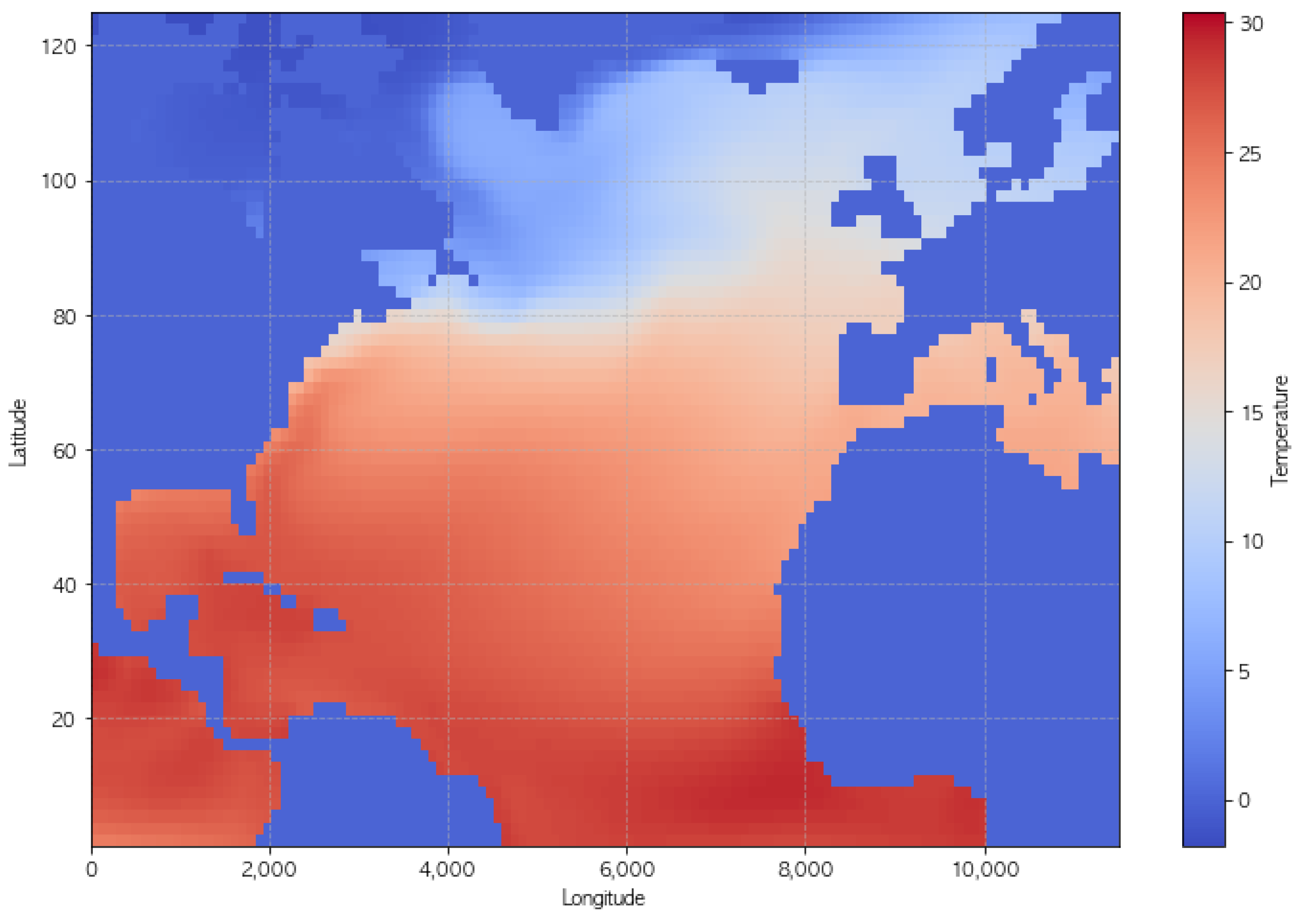
For the climate datasets, we analyze two distinct but related spatiotemporal datasets derived from the Community Earth System Model (CESM2) pre-industrial control experiment: a global surface air temperature dataset and a North Atlantic sea surface temperature (SST) dataset [42]. These datasets enable the evaluation of our model’s capacity to capture complex climate system dynamics under controlled conditions. Samples of projected worldwide maps are depicted in Figure 5 and Figure 6.

The global temperature dataset consists of monthly averaged fields spanning 1200 years, with a spatial resolution of 192 × 288 grid points (latitude × longitude), resulting in a data tensor of shape (14,389 × 192 × 288). The input data have been preprocessed to remove the climatological seasonal cycle, focusing on deviations that represent internal climate system variability. The normalized temperature data show a near-zero mean of $4.097\times {10}^{-5}$ with a standard deviation of 0.708, reflecting the successful removal of systematic seasonal variations. The spatial coordinates are represented by latitude arrays (shape: 192) and longitude arrays (shape: 288), providing complete global coverage.

The North Atlantic SST dataset (ToSNA) focuses on a specific region with dimensions (14,389 × 70 × 125), representing 800 years of monthly data at a nominal 1° horizontal resolution. The data have been carefully curated to maintain scientific validity, with no missing values (NaN count: 0) and a temperature range from −1.80 °C to 30.41 °C, with a mean of 11.28 °C. To isolate internal climate variability, we employed two key preprocessing steps: (1) removing the time-mean SST at each geographical location to eliminate latitudinal variation and (2) applying a 12-month moving average at each location to remove the seasonal cycle. Specifically, we focused on capturing internal climate system dynamics. To ensure robust evaluation, we maintained temporal coherence when splitting the dataset into training and validation sets, allowing the model to learn and validate complex Earth system dynamics, keeping climate patterns and oscillations.

However, this sequential splitting method introduces some potential limitations. Since the validation and test sets are not randomly sampled, strong temporal correlations in climate data might lead to overfitting, where the model adapts too closely to patterns in the training data. This could result in overly optimistic performance metrics.

4.4. Evaluation Metrics

We utilize three primary metrics—MSE, PSNR, and SSIM—to evaluate the performance of the models. Each metric provides a unique perspective on assessing the similarity between the predicted and ground-truth frames.

MSE (mean squared error) measures the average squared difference between the predicted and ground-truth frames. A lower MSE indicates that the predicted frame is closer to the actual frame. MSE is defined as follows:

$$\mathrm{MSE}={\displaystyle \frac{1}{mn}}\sum _{i=1}^m\sum _{j=1}^n{\left(I_{ij}-{\widehat{I}}_{ij}\right)}^2,$$

where $I_{ij}$ represents the pixel value of the ground-truth frame, ${\widehat{I}}_{ij}$ is the pixel value of the predicted frame, and m and n denote the height and width of the frame, respectively. MSE is selected as it provides a basic and intuitive measure of pixel-level accuracy, making it suitable for evaluating the overall regression performance of the model.

The PSNR (Peak Signal-to-Noise Ratio) is derived from MSE and represents the ratio between the maximum possible power of a signal and the power of noise on a logarithmic scale. A higher PSNR indicates that the predicted frame has a higher similarity to the ground-truth frame. The PSNR is defined as

$$\mathrm{PSNR}=10·{log}_{10}\left({\displaystyle \frac{MA{X}^2}{\mathrm{MSE}}}\right),$$

where $MAX$ is the maximum possible pixel value of the image (e.g., $MAX=255$ for 8-bit images). The PSNR complements MSE by emphasizing the perceptual quality of the image. The PSNR is chosen as it emphasizes signal quality and is widely used for image quality evaluation, complementing MSE by providing a perceptual perspective.

The SSIM (Structural Similarity Index Measure [43]) measures the structural similarity between the predicted and ground-truth frames by considering luminance, contrast, and structural information. The SSIM measures image similarity on a scale of 0 to 1, with 1 indicating identical images. The SSIM is calculated as follows:

$$\mathrm{SSIM}(I,\widehat{I})={\displaystyle \frac{(2{\mu }_I{\mu }_{\widehat{I}}+C_1)(2{\sigma }_{I\widehat{I}}+C_2)}{({\mu }_I^2+{\mu }_{\widehat{I}}^2+C_1)({\sigma }_I^2+{\sigma }_{\widehat{I}}^2+C_2)}},$$

where ${\mu }_I$ and ${\mu }_{\widehat{I}}$ represent the mean pixel values of the ground-truth frame I and the predicted frame $\widehat{I}$, ${\sigma }_I^2$ and ${\sigma }_{\widehat{I}}^2$ denote the variances of the ground-truth and predicted frames, respectively, ${\sigma }_{I\widehat{I}}$ indicates the covariance between I and $\widehat{I}$, and $C_1$ and $C_2$ are small constants used to stabilize the division. The SSIM is included as it evaluates structural similarity, providing a better correlation with the human perception of image quality compared to MSE and the PSNR.

The SSIM is particularly effective for assessing image structural similarity, often correlating better with human perceptual quality than the PSNR or MSE alone. Each of these metrics provides a different lens through which the quality of the predicted frames can be analyzed and helps to comprehensively assess how well the proposed model approximates the ground-truth frames.

In addition to these metrics, we also included the Kolmogorov–Smirnov (KS) test to quantitatively compare the pixel distributions between the ground-truth and predicted frames. The KS test measures the maximum difference between the cumulative distribution functions (CDFs) of two datasets, providing a statistical basis for evaluating whether the predicted frames faithfully reproduce the ground-truth distribution. The KS statistic is calculated as follows:

$$D=\underset{x}{sup}\left|F_{\mathrm{GT}}\left(x\right)-F_{\mathrm{Pred}}\left(x\right)\right|,$$

where $F_{\mathrm{GT}}\left(x\right)$ and $F_{\mathrm{Pred}}\left(x\right)$ are the CDFs of the ground-truth and predicted pixel values, respectively. A smaller KS statistic indicates that the two distributions are more similar. We report both the KS statistic and the associated p-value, with $p<0.05$ indicating a statistically significant difference between the distributions.

The KS test provides additional insights into the fidelity of the predicted frames, particularly in terms of their ability to replicate the statistical properties of the ground-truth frames. The KS test is added to assess the statistical fidelity of the predicted frames, offering insights into how well the model reproduces the pixel distribution of the ground truth. This complements traditional metrics by highlighting differences in data distribution. By incorporating this test, we aim to offer a comprehensive evaluation framework that extends beyond traditional pixel-level metrics.

5. Results

We evaluated our bidirectional approach with the dynamic window size adaptation using the SSIM and MSE.

Table 1. Comparison of model performance across different datasets.

Model	MSE	PSNR	SSIM
Moving MNIST Dataset (10 time steps)
FC-LSTM	118.30	27.40	0.69
ConvLSTM	103.30	27.99	0.71
PredRNN	56.80	30.59	0.87
PredRNN++	50.70	31.08	0.89
Bidirectional PredRNN	49.25	31.21	0.89
Bidirectional PredRNN + Dynamic Window Size	47.60	31.34	0.90
KTH Dataset (10 time steps)
ConvLSTM	285.15	23.58	0.71
PredRNN	114.31	27.55	0.84
PredRNN++	92.49	28.47	0.87
Bidirectional PredRNN	98.79	29.16	0.75
Bidirectional PredRNN + Dynamic Window Size	91.28	29.25	0.88
ToSNA Dataset (30 frames)
ConvLSTM	60.30	26.32	0.78
PredRNN	51.40	27.02	0.82
Bidirectional PredRNN	49.60	27.18	0.83
Bidirectional PredRNN + Dynamic Window Size	48.25	27.29	0.84
Climate Dataset (30 frames)
ConvLSTM	45.20	27.10	0.78
PredRNN	40.35	27.80	0.80
Bidirectional PredRNN	38.50	28.20	0.81
Bidirectional PredRNN + Dynamic Window Size	37.25	28.60	0.82

Lower values are better for MSE, and higher values are better for PSNR and SSIM.

presents a comparative analysis of our model against state-of-the-art PredRNN approaches. The SSIM provides a comprehensive assessment of structural similarity between predicted and ground-truth frames, ranging from −1 to 1, with higher scores indicating better prediction quality. Table 1 presents a comparative analysis of our model against state-of-the-art approaches. Notably, we include the baseline PredRNN model (Wang et al., 2018 [17]) to demonstrate the impact of our bidirectional memory flow and dynamic window mechanism.

Our experimental results show that the adaptive window size mechanism, which ranges from $w_{min}=3$ to $w_{max}=11$ frames, effectively captures both short-term and long-term dependencies in the sequence. The dynamic window, governed by our optical flow estimator and EMA smoothing ($\alpha =0.8$), balances computational efficiency and prediction accuracy by dynamically adjusting between short-term ($w_{min}$) and long-term ($w_{max}$) dependencies based on temporal dynamics. For the 10-frame prediction task, our model achieves comparable performance to existing approaches, particularly in sequences with varying motion intensities. This suggests that our bidirectional architecture can effectively leverage both past and future contexts through its dynamic window adaptation.

We extended the prediction horizon from 10 to 30 frames to evaluate the temporal prediction limits of our model. While the model maintains competitive performance in terms of SSIM and MSE metrics for longer sequences, the performance begins to degrade as the dynamic window size approaches its upper limit ($w_{max}$), particularly in datasets with high motion complexity. This degradation illustrates the limitations of capturing extended dependencies with fixed upper bounds in the temporal horizon, emphasizing the importance of appropriately defining such boundaries. Based on these observations, we focus our subsequent analysis on the 10-frame prediction task, where our model demonstrates more stable and reliable performance.

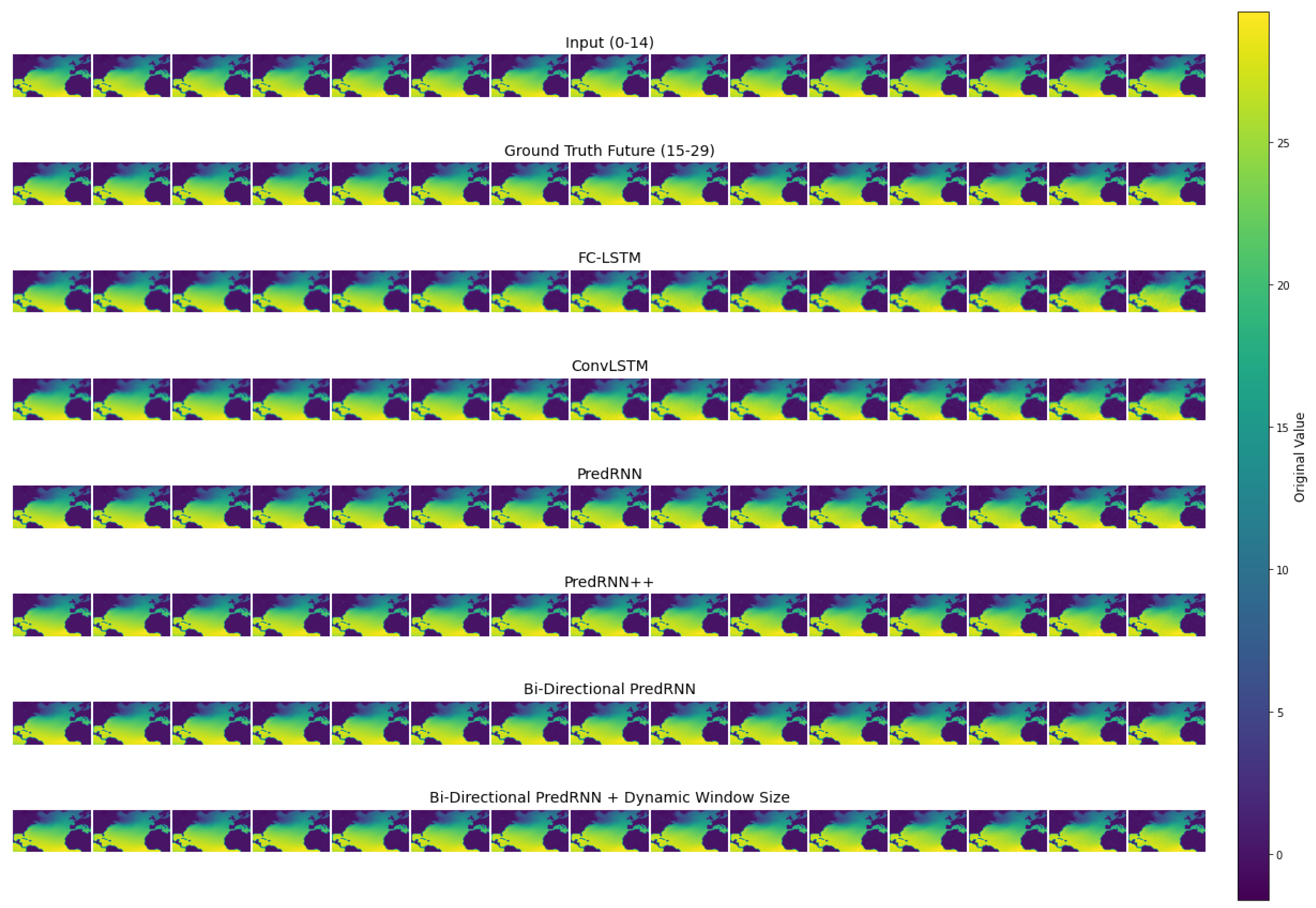
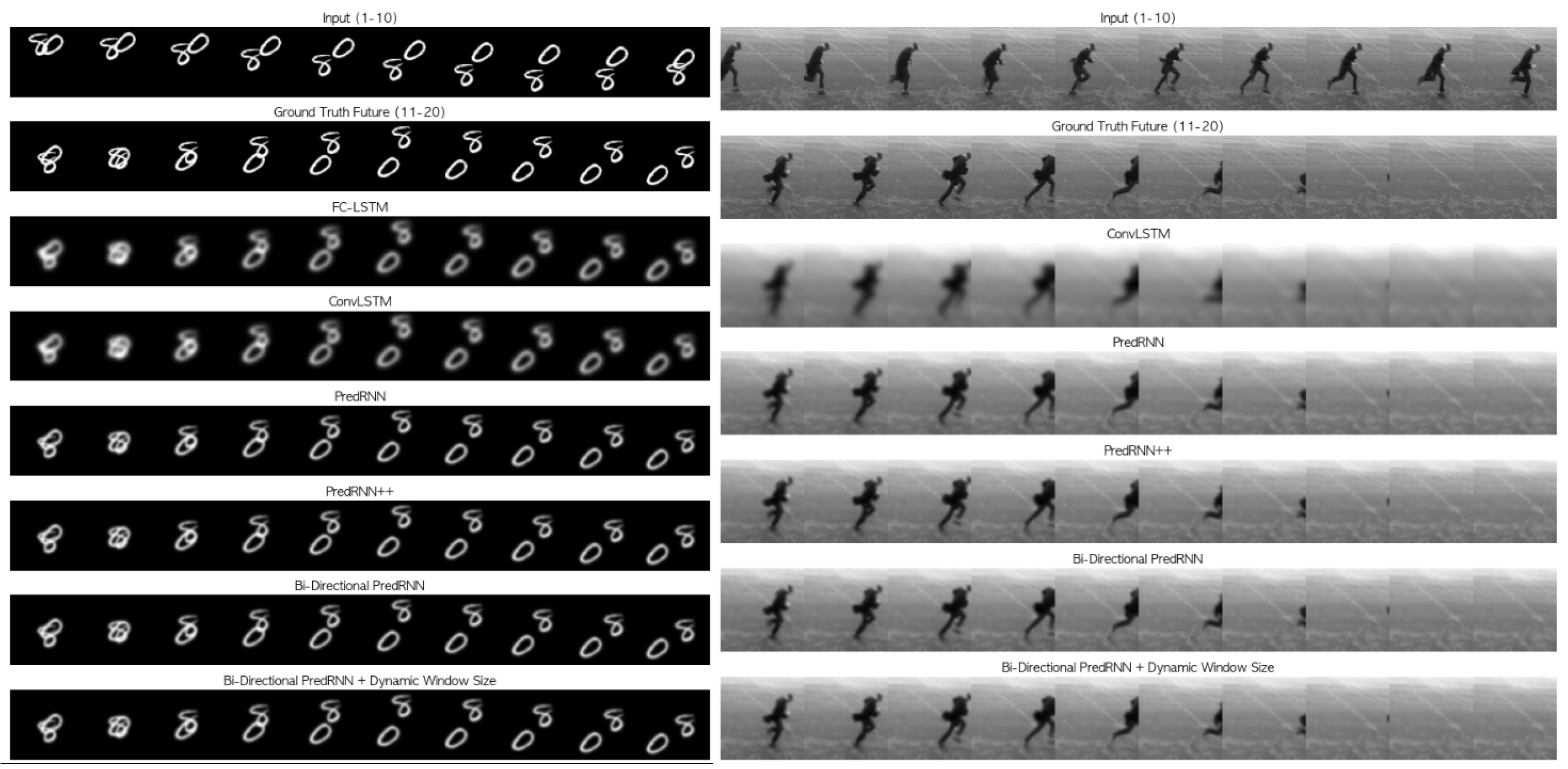
In Figure 7, we present examples of predicted frames that demonstrate the superior performance of our Bidirectional PredRNN model with dynamic window size adaptation. The quantitative results show that our model achieves better performance across all metrics on the Moving MNIST dataset (MSE: 47.60, PSNR: 31.34, SSIM: 0.90) compared to existing approaches, including PredRNN++ (MSE: 50.70, PSNR: 31.08, SSIM: 0.89).

When evaluating our model’s performance on the KTH Action dataset, we observe an interesting pattern. The basic Bidirectional PredRNN shows slightly degraded performance (SSIM: 0.75) compared to PredRNN++ (SSIM: 0.87), which can be attributed to the increased complexity of human motion patterns and the potential overfitting of the bidirectional architecture to local temporal dependencies. However, with the introduction of our dynamic window size adaptation mechanism, the model significantly improves its performance (MSE: 91.28, PSNR: 29.25, SSIM: 0.88), surpassing PredRNN++ in PSNR metrics and achieving comparable SSIM scores.

For the ToSNA dataset, our model shows steady improvement over baseline approaches, with the dynamic window size adaptation mechanism further enhancing prediction accuracy (MSE: 48.25, PSNR: 27.29, SSIM: 0.84) compared to the conventional ConvLSTM (MSE: 60.30, PSNR: 26.32, SSIM: 0.78). Regarding the climate dataset, while our model shows promising results (MSE: 37.25, PSNR: 28.60, SSIM: 0.82) and outperforms existing approaches, it is important to note some methodological considerations. Unlike traditional validation approaches, the climate dataset was processed sequentially due to its temporal nature, with later time periods serving as test data. This sequential splitting method was chosen to preserve the natural progression of time in climate data, which is critical for maintaining the integrity of temporal dependencies inherent in such datasets.

However, data augmentation, which is commonly used to expand datasets and enhance model generalization, poses unique challenges in the context of climate data for several reasons. First, augmenting climate data risks introducing artifacts that can contaminate the physical authenticity of the data, particularly when simulating phenomena like convection or fluid-dynamic interactions, which follow strict natural laws. Second, climate systems are significantly influenced by external events, such as ice ages or anthropogenic climate change. These catastrophic or external factors introduce variability that is not strictly endogenous to the climate system itself. Consequently, ensuring sequential integrity and standalone datasets is essential to effectively capture the underlying system dynamics without conflating external influences.

While this approach allows for more realistic modeling, it also introduces potential risks of overfitting, as the validation set is not randomly sampled but derived from later periods. Future work could explore validation strategies that balance the need for temporal coherence with the benefits of broader sampling, such as temporal slicing or incorporating domain-specific regularization techniques to account for strong temporal correlations in the data.

We further investigated the statistical and visual differences in the generated results by comparing the pixel value distributions, cumulative distribution functions (CDFs), and Kolmogorov–Smirnov (KS) statistics of the models. In Figure 8, the left panel shows the pixel value distributions of both models compared to the ground truth. PredRNN++ deviates more from the ground truth, particularly in the lower-intensity range, where the pixel values are concentrated. In contrast, Bi-PredRNN closely matches the ground-truth distribution, indicating that it better represents the actual pixel value characteristics.

The middle panel presents the cumulative distribution functions (CDFs) of the models and the ground truth. Bi-PredRNN exhibits a smaller deviation from the ground-truth CDF compared to PredRNN++, especially in the middle-intensity range (50–150). This observation is supported by the KS statistic in

Table 2. Comparison of KS test results and distribution statistics on Moving MNIST dataset.

Model	KS Statistic	p-Value	Mean (GT)	Std (GT)	Mean (Model)	Std (Model)
PredRNN++	0.2646	$4.43\times {10}^{-209}$	11.55	48.68	10.45	41.48
Bi-PredRNN	0.0952	$5.78\times {10}^{-162}$	11.55	48.68	11.18	40.16

GT refers to ground truth, KS statistic represents the maximum difference in cumulative distributions, and p-value indicates the statistical significance of the difference.

, where Bi-PredRNN achieves a lower value (0.0952) than PredRNN++ (0.2646). The smaller KS statistic indicates that Bi-PredRNN’s predictions are statistically more similar to the ground truth.

The right panel highlights the KS statistic as a function of pixel values, with the red dashed line representing the maximum difference between the CDFs of the ground truth and the models. PredRNN++ shows a larger peak in the low-intensity range, indicating a greater deviation from the ground truth. On the other hand, Bi-PredRNN demonstrates a more consistent and lower deviation across pixel values, showing the benefits of bidirectional processing for capturing the true data distribution.

These results confirm that Bi-PredRNN not only improves pixel-wise accuracy and structural similarity, as shown in MSE and SSIM metrics, but also replicates the statistical properties of the ground-truth distribution more accurately. These results confirm that Bi-PredRNN improves both prediction accuracy and alignment with the ground-truth distribution, as demonstrated by the MSE, SSIM, and KS metrics.

Qualitative Works

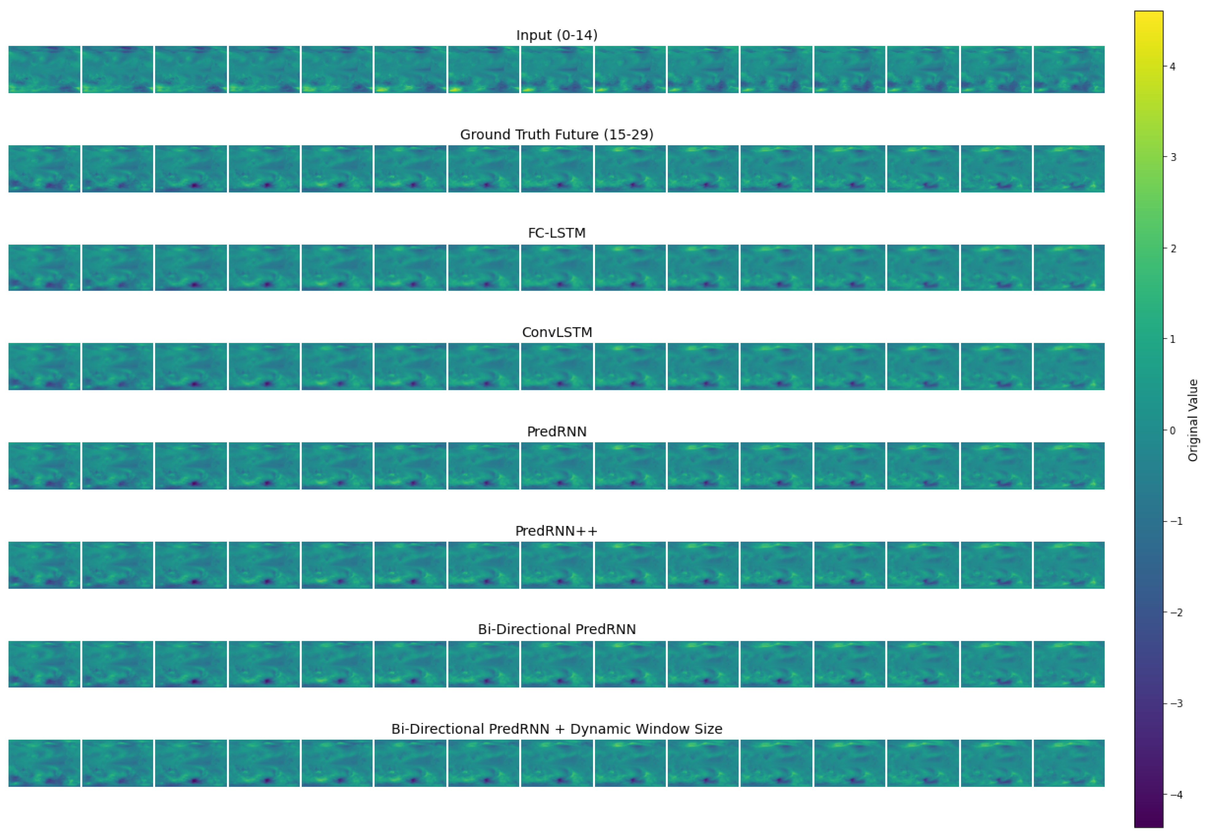
In Figure 7, we analyze the qualitative performance of our Bidirectional PredRNN model with dynamic window size adaptation across both Moving MNIST and KTH Action datasets. For Moving MNIST sequences, our model maintains sharp digit boundaries and preserves distinctive numerical features (e.g., the curve in ‘0’, ‘8’) without distortion. The model accurately predicts the trajectory changes when digits collide, and it demonstrates physically plausible reflection patterns at frame boundaries.

The KTH Action sequences show our model’s capability to handle complex human motion patterns. The dynamic window size adaptation mechanism is particularly effective for the capture of natural human movements because it automatically adjusts the temporal receptive field based on motion complexity. The results show smooth and continuous predictions of coordinated body movements, from the synchronized motion of arms and legs during walking to precise finger movements in hand-waving actions. Our model consistently maintains temporal coherence and preserves subtle details such as clothing folds and shadow interactions under various lighting conditions.

For the ToSNA and climate datasets, which track 14,389 years of temperature changes, their design makes them well suited for measuring fluid-thermodynamic variability. However, the low standard deviation, particularly in the climate dataset (0.708), poses challenges for visualization in a static, paper-based medium. This limitation underscores the importance of incorporating dynamic representations such as animations or interactive visualizations to effectively convey the subtle variations within these datasets. To address this, we have included supplementary visualizations for both datasets in the appendix (for the ToSNA dataset, refer to Figure A1, and for the climate dataset, refer to Figure A2).

6. Conclusions

We have tackled key challenges in spatiotemporal sequence prediction, focusing on the difficulties of capturing complex temporal dependencies and preserving spatial coherence in long sequences. Traditional models often struggle with these tasks due to the vanishing gradient problem and limitations in maintaining spatial information over time. Bi-PredRNN extends PredRNN by incorporating bidirectional processing capabilities to address these challenges.

Our primary contribution is a bidirectional memory network architecture that processes temporal information in both the forward and backward directions, with specialized memory cells to ensure spatial coherence. We have also introduced a dynamic window size mechanism, which adapts temporal context based on optical flow estimation and EMA smoothing, allowing for more flexible temporal processing. Experimental results across diverse datasets highlight the robustness and versatility of our model. On Moving MNIST, Bi-PredRNN demonstrates significantly improved prediction accuracy by effectively capturing intricate spatiotemporal patterns. For KTH Action, the model exhibits enhanced stability in preserving long-term dependencies, which are essential for reliable action prediction. Additionally, on climate data, our approach outperforms traditional unidirectional models in forecasting long-range temporal patterns, underscoring its applicability to real-world challenges.

While our model shows promising results, challenges remain in handling uncertain temporal dependencies. While bidirectional processing enriches temporal context, it can introduce uncertainty when future states significantly influence past interpretations. For instance, in chaotic or highly dynamic systems, the bidirectional mechanism may lead to spurious correlations between future and past states, complicating the model’s ability to maintain causal integrity. These limitations highlight the need for advanced temporal attention mechanisms that dynamically adjust the weight of past and future contexts based on their relative importance. Hybrid architectures, which adapt between unidirectional and bidirectional processing depending on the temporal characteristics of the sequence, also represent a promising direction for mitigating these challenges.

Bidirectional networks demonstrate their greatest strength in domains where sequential relationships are explicit and context plays a critical role, such as in natural language processing. In NLP tasks, bidirectional models excel by leveraging contextual cues from subject–predicate relationships or subsequent modifiers to achieve outstanding performance. This explains why bidirectional architectures are particularly effective for sentence-level tasks where word dependencies are clearly defined within datasets. However, when applied to spatiotemporal data, especially video-based datasets, where the nature of correlations between vectors differs from word vectors, the consistency of such performance is less substantiated.

Therefore, tailoring the network to specific domain knowledge could further reduce temporal uncertainty in particular applications, enhancing the model’s performance in broader contexts. By integrating these advancements, future iterations of Bi-PredRNN could achieve greater reliability and accuracy across diverse spatiotemporal prediction tasks.