A Multiscale Adaptive Fusion Network for Modular Multilevel Converter Fault Diagnosis

Abstract

Modular Multilevel Converters (MMCs) play a crucial role in new energy grid connection and renewable energy conversion systems due to the significant merits of good modularity, flexible scalability, and lower operating loss. However, reliability is a significant challenge for MMCs, which consist of a large number of Insulated Gate Bipolar Transistors (IGBTs). Failures of the IGBTs in submodules (SMs) are a critical issue that affect the performance and operation of MMCs. The insufficient ability of convolutional neural networks to learn key fault features affects the accuracy of MMC fault diagnosis. To resolve this issue, this paper proposes a novel deep fault diagnosis framework named the Multiscale Adaptive Fusion Network (MSAFN) for MMC fault diagnosis. In the proposed MSAFN, the fault features of the raw current in an MMC are extracted by employing multiscale convolutional neural networks (CNNs) firstly, and then a channel attention mechanism is added to adaptively select the channel containing key features, so as to improve the fault diagnosis ability of the MMC in a noisy environment. Finally, the adaptive size of a one-dimensional CNN is adopted to adjust the weight of the feature channels of different scales, which are adaptively fused for fault diagnosis. Experimental validation is performed on two different MMC datasets. Experimental results confirm that the introduction of an attention mechanism of the multiscale feature adaptive fusion channel improves the recognition accuracy of the model by an average of $15.6\%$. Moreover, comparative experiments under different signal-to-noise ratios (SNRs) demonstrate that the MSAFN maintains accuracy levels above $96.7\%$, highlighting its excellent performance, particularly under noisy conditions.

1. Introduction

Over the past few years, Modular Multilevel Converters (MMCs) have been extensively utilized in new energy grid connection and renewable energy conversion systems as well as high-voltage applications. This is attributed to its modular structure, ease of scalability, superior low harmonic content, minimal operating loss, and the presence of a shared DC-Link [1,2,3]. Each basic unit of an MMC is a submodule (SM), which consists of a power device and a capacitor device. Therefore, this converter structure does not require direct series connection of devices, but instead achieves the purpose of outputting various levels of voltage and power through different numbers of submodules that are cascaded. This has advantages such as low harmonic content, good scalability, strong modularity, and easy scalability to any level. Despite the above advantages, it is known that the operational continuity of the MMC is susceptible to disruption on account of the fragility of the semiconductor switch components, which are recognized as amongst the most delicate elements within power conversion systems. This is especially true for MMCs, given that practical MMC systems always incorporate a substantial quantity of Insulated Gate Bipolar Transistors (IGBTs), often dozens or even hundreds, which highlights that IGBTs are the components most prone to developing failures [4,5]. Therefore, the reliability of MMC systems is a critical challenge. When an IGBT encounters an open-circuit (OC) fault, the capacitor voltage in the affected MMC SM continues to rise, leading to distortion in both the output voltage and current of the MMC. Without effective fault diagnosis methods, this issue can ultimately result in MMC shutdowns or even physical damage, compromising the stability of the power grid. Thus, research on fast and accurate fault diagnosis and localization technology is of great significance for the safe operation of MMC systems [6,7,8].

In recent times, the focus on fault diagnosis in MMCs has grown significantly. In general, research on MMC fault diagnosis has mainly focused on two aspects: model-based and data-driven diagnosis [9,10,11,12]. The physical model-based fault diagnosis method utilizes the structure and working principle of an MMC to develop a mathematical model, and determines the existence of faults by comparing the differences between the actual operating data and theoretical models. The advantage of this method is that it can provide accurate fault location and diagnosis results, but it requires accurate model parameters and complex calculation processes. The data-driven fault diagnosis method collects the operating data of the MMC system and uses techniques such as machine learning and data mining to analyze and diagnose faults. This method has the characteristics of strong real-time performance and good adaptability, but for large-scale MMC systems, data processing and analysis are relatively complex [13,14,15].

In recent years, deep learning-based fault diagnosis, a leading data-driven approach, has demonstrated remarkable effectiveness in automatically extracting features from large datasets and adeptly addressing complex diagnostic challenges [16,17,18,19,20,21,22]. Among them, the Convolutional Neural Network (CNN) utilizes the idea of a convolutional operation to significantly decrease the number of model parameters while enhancing the network’s ability, achieving end-to-end intelligent diagnosis without the need for signal preprocessing [23]. In [24], A fault diagnosis method based on an improved capsule network (CapsNet) is proposed for an MMC compound fault; this feature extraction structure of the network combines the light weight of 1DCNN and the sequential sensitivity of LSTM. In [25], a CNN model is developed for detecting and locating structural damage in rotating machinery. Although the CNN performs well in extracting bearing fault features, it has difficulty in extracting fault features in the presence of noise interference, leading to a decrease in diagnostic accuracy. Zhai et al. [26] proposed a domain-adaptive CNN model with good diagnostic results in noisy environments with signal-to-noise ratios (SNRs) ranging from 0 dB to 10 dB. Zhang et al. [27] developed a deep CNN with a wide convolutional kernel as the first layer to extract bearing fault features, which can still perform bearing fault diagnosis in noisy environments with an SNR of −4 dB to 10 dB.

Traditional CNN fault diagnosis models extract bearing fault features at a single scale or by deepening the network layers, while rolling bearing vibration signals have complex time-scale features [28]. If a fixed size convolution is used, other time-scale features cannot be obtained. Using multiscale convolution can learn features at different time scales, which helps convolutional neural networks recognize fault features.

Ma et al. [29] proposed a multiscale convolutional neural network that can effectively learn advanced fault features. But after obtaining features at different scales, it involves just a simple concatenation without considering the differences in features at different scales. In [30], a multiscale convolutional neural network is developed with an SNR of 0 dB to 6 dB. In [31], Xu et al. introduced a multiscale CNN for parallel learning, which has high fault diagnosis accuracy in noisy environments with an SNR of −4 dB to 12 dB.

Although the above research uses multiscale convolution to extract features at different scales, there are still the following issues: (1) In traditional CNNs, a large number of channels are often used to enhance feature representation. Although such deep CNNs can improve performance, not all channels carry valuable fault information, and some channels may even learn noise distribution features. Treating all channels indiscriminately not only increases the structural complexity of the CNN but also results in wasted computational resources. (2) Fault characteristic frequency components and interference components in signals are distributed across different scales, and variations in operating conditions can affect this distribution. Consequently, the diagnostic value of information at different scales is not equivalent. Although existing multiscale CNNs employ multiple convolution paths to capture information at various scales, they often fail to fully account for inter-scale differences, making them susceptible to irrelevant components and redundant information [32]. (3) Most multiscale convolutional neural networks only connect features of different scales and link them with fully connected layers for classification, without considering the differences in the features of different scales, resulting in reduced accuracy of fault diagnosis.

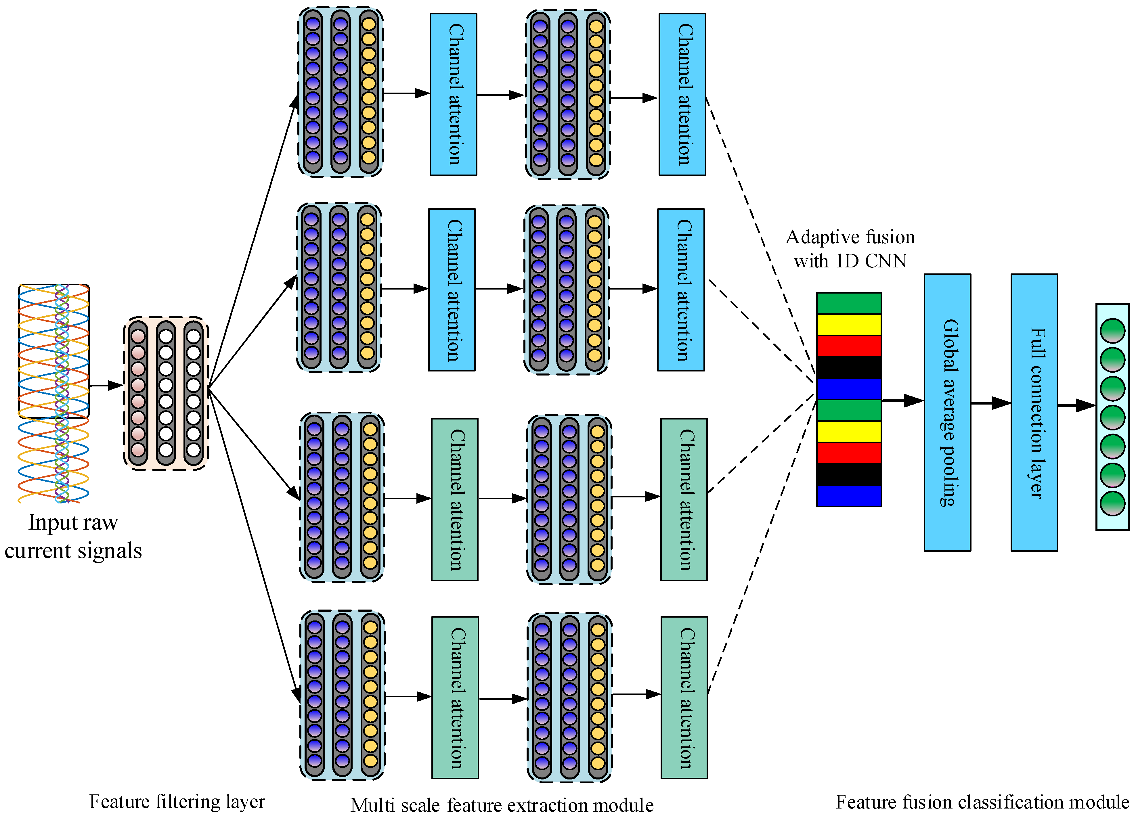
Motivated by the preceding discussion, a new deep fault diagnosis framework named the Multiscale Adaptive Fusion Network (MSAFN) is introduced in this paper. Firstly, a wide convolutional layer is utilized to filter features from the raw output and internal circulating current signal of the MMC. Then, fault features are extracted from convolutions of different scales. Then, channel attention is used to adjust the channel weights of different features, select effective fault features for learning, reduce the impact of invalid features, suppress noise interference, and finally, use adaptive 1D convolution in the feature fusion layer for adaptive fusion. The major contributions of the paper are highlighted as follows: (1) A wide convolution layer is employed to filter features from both the original output current and the internal circulating signal, followed by multiscale convolution to extract fault features. Channel attention is then applied to adjust the weights of the different feature channels, enabling the model to select effective fault features and enhancing its diagnostic performance in noisy environments. (2) Building on a multiscale CNN architecture, the model’s capability to capture features at various scales is enhanced. Data across multiple scales are treated as large channels, and an adaptive 1D convolution is employed in the feature fusion layer to achieve effective multiscale feature integration. (3) During model training, a Cyclical Learning Rate (CyclicLR) strategy is used to dynamically adjust the learning rate, which helps the model avoid premature convergence to local optima and improves its generalization capability. (4) The proposed MSAFN model has been extensively evaluated on 11-level and 31-level MMC datasets. Experimental results confirm that MSAFN achieves optimal fault diagnosis performance even in noisy environments.

The remaining sections of this paper are organised as follows: In Section 2, we concisely introduce the topological structure and SM fault analysis of an MMC. Section 3 describes the multiscale convolutional neural network model, and explains the methodological framework used in this study in detail. Section 4 shows the experimental results and compares the effectiveness of the proposed methods. Finally, Section 5 summarizes the main points of this paper.

2. MMC Topology and Submodule Fault Analysis

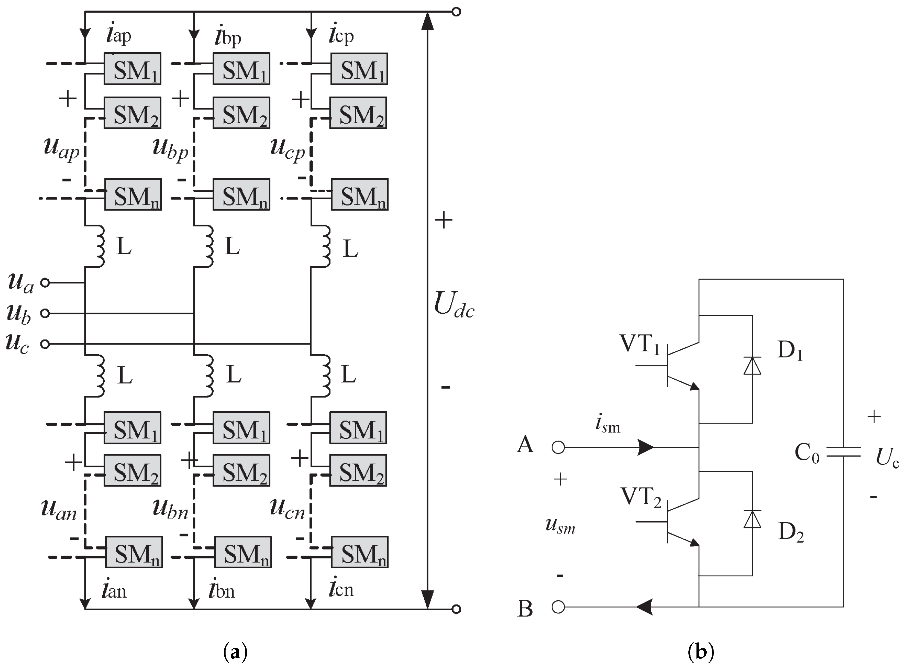
The main topological structure of an MMC is divided into three phases, each comprising upper and lower bridge arms, as shown in Figure 1a. Each bridge arm contains the same number of SM units in series. The SM is the basic power unit that constitutes the MMC. The half-bridge submodule (HBSM) is widely used because of its simple structure, convenient control, and low cost. Each HBSM includes two IGBTs, $V{T}_1$ and $V{T}_2$, two reverse parallel diodes, $D_1$ and $D_2$, and a floating capacitor, C, as shown in Figure 1b.

The total number of conductive SMs in each phase unit of MMC should comply with Equation (1), which is as follows:

$$U_{dc}=N{U}_c$$

(1)

where $U_{dc}$ is the DC voltage of the MMC DC-Link, N is the number of SMs connected in series per bridge arm, and $U_c$ is the capacitance voltage of the DC side per SM.

Using any phase as an example, the currents of the upper and lower bridge arms are displayed below.

$$\begin{array}{c}\left\{\begin{array}{c}\begin{array}{c}{i}_{jp}=(-i_j/2)+i_{dc}/3+i_{diff.j}(j=a,b,c)\hfill \\ i_{jn}=(i_j/2)+i_{dc}/3+i_{diff.j}(j=a,b,c)\hfill \end{array}\hfill \end{array}\right.\hfill \end{array}$$

(2)

where $i_{jp}$ and $i_{jn}$ are the upper and lower arm currents, $i_{dc}$ is the DC side current, and $i_j$ is the output current of MMC.

Considering Equation (2), the equation for the circulating current can be expressed as follows:

$$\begin{array}{c}\hfill i_{diff.j}=(i_{pj}+i_{nj})/2(j=a,b,c)\end{array}$$

(3)

where $i_{diff.j}$ is the internal circulating current.

Each HBSM in an MMC contains two IGBTs, which are the most vulnerable components and prone to failure. IGBT failures can be mainly categorized into two types: open-circuit (OC) faults and short-circuit (SC) faults. In the power system, SC faults are highly destructive and there are well-established solutions for SC faults. Nevertheless, due to the unclear characteristics of IGBT OC faults, they are challenging to detect, and the prolonged operation of power equipment with such faults can cause significant damage. Although OC faults do not result in an immediate system collapse, they lead to increased harmonic content, which degrades the quality of the power supply and system performance. Consequently, this article mainly focuses on diagnosing IGBT OC faults in MMCs.

An OC fault in an MMC alters the current flow path within the SM, impacting both the MMC’s output and the internal circulating currents. This type of fault causes distortion in the waveforms of both the output and circulating currents. The impact of IGBT OC faults varies depending on the phase and bridge arm involved [33]. Taking these factors into account, this paper employs the waveforms of the output current and circulating currents in the MMC as diagnostic indicators for fault detection.

3. Multiscale Convolutional Neural Network Model

3.1. Convolutional Neural Network

CNNs are among the most effective multi-hidden-layer deep learning models, which convert low-level features into high-level features through hierarchical feature transformation, and which can effectively achieve feature learning and expression. CNNs mainly include convolutional layers, pooling layers, dense layers, and classifier layers. At the front end of the network, several convolutional and pooling layers are stacked to learn the underlying features of the input signal. The dense layer then transforms the two-dimensional feature vectors into one-dimensional vectors. Finally, fault diagnosis is carried out at the classifier layer at the back end of the network.

The convolutional layer is the most important layer in the entire CNN. Its structure is different from that of the dense layers, where the input of each node in the convolutional layer is only connected to a portion of the neurons in the preceding layer. The output from a subset of nodes in the neural network layer preceding the convolution layer serves as the input for each node in the convolution layer, usually implemented by the convolutional kernel. The main function of the convolutional layers is to perform convolutional operations, which can be understood as feature extraction for each small pixel in an image. For the input feature mapping data, convolution operations slide the filter window at certain intervals and apply it. The filter elements are multiplied at each position with the corresponding input elements, and then are summed. This process can be expressed as Equation (4)

$$\begin{array}{c}\hfill {\mathit{y}}_j^l=\mathit{f}(\sum _{i\in M_j}^N{x}_i^{l-1}\ast w_{ij}^l+b_j^l)\end{array}$$

(4)

where ${\mathit{y}}_j^l$ represents the $jth$ output of the layer l, $x_i^{l-1}$ represents the $jth$ input of the layer l. $M_j$ is the $jth$ convolutional region of the layer $l-1$, $w_{ij}^l$ represents the weight of the convolutional kernel, $b_j^l$ is the bias vector. The * symbol represents the convolution operator; $f(·)$ is the activation function, N is the number of convolutional kernels.

The features obtained after convolution generally need to be downsampled through pooling layers for feature selection and information filtering, which can effectively prevent overfitting. Both average pooling and maximum pooling can be used, though maximum pooling is widely utilized in practice. Its calculation equation is as follows:

$$\begin{array}{c}\hfill {\mathit{P}}_j^l=\mathit{max}\left(x_j^l\right)\end{array}$$

(5)

where ${\mathit{P}}_j^l$ is the final output of layer l, and $x_j^l$ is the corresponding maximum pooling of the $lth$ region.

After processing several rounds using convolutional and pooling layers, typically one to two dense layers will provide the final classification result at the end of the CNN. After multiple rounds of convolution and pooling, the original information is abstracted into features with greater informational content. Therefore, the role of the convolutional and pooling layers in CNN can be understood as the process of automatically extracting features. After extracting the features, a dense layer is used to complete the fault detection task. The calculation formula for the output vector of the dense layer is as follows:

$$\begin{array}{c}\hfill {\mathit{q}}_j^l=\sigma (\sum _i{x}_i^{l-1}\ast {\omega }_{ij}^l+c_j^l)\end{array}$$

(6)

where ${\mathit{q}}_j^l$ represents the $jth$ characteristic value of the $ith$ data in the $lth$ layer, ${\omega }_{ij}^l$ is the weight of the $jth$ output value, $c_j^l$ is the bias vector, $\mathit{\sigma }(·)$ is the activation function.

For multi-classification problems, by selecting the activation function of the last dense layer of the network as $sotmax$ and the number of neurons as the number of multi-classifications, multi-category tasks can be directly completed. The calculation equation is as follows:

$$\begin{array}{c}\hfill p\left(i\right)={\displaystyle \frac{{\mathit{e}}^{x_j}}{{\sum }_{j=1}^K{\mathit{e}}^{x_j}}}\end{array}$$

(7)

where K is the number of classification categories, $x_j$ is the j-th feature, and $p\left(i\right)$ is the probability that $x_j$ belongs to the $jth$ category.

3.2. Channel Attention Mechanism

With the aim of solving the problem of unequal information value between a large number of channels in convolutional neural networks, which makes it difficult to train the network and affects recognition accuracy, this paper introduces the channel attention mechanism method proposed in [16] and improves it. This method compresses global information into the dimension of information channels through mean pooling and maximum pooling, thereby establishing interdependence relationships between different channels. In order to further obtain the criticality of different channels, the pooled vectors are fed into the bottleneck structure’s squeeze excitation network, and the compression ratio r is set to force the network to discard some unimportant neuron values.

The core component of SEnet is the SE (Squeeze and Excitation) block, which mainly consists of Squeeze and Excitation parts, as shown in Figure 2.

Each channel of an ordinary CNN learns in its local receptive field and cannot use the context information of other channels. For this reason, the Squeeze network obtains the characteristic diagram X through convolution, and then obtains the global information z by compressing the characteristic diagram X through GAP (GlobalAverage Pooling). $z_c$ is the c th element of z, and its calculation formula is as follows:

$$\begin{array}{c}\hfill z_c=F_{sq}\left(u_c\right)={\displaystyle \frac{1}{H\times W}}\sum _{i=1}^H{u}_{c(i,j)}\end{array}$$

(8)

where $u_c$ is the $c\text{-}th$ channel of X, and H and W are the height and width of the input characteristic graph.

After Excitation, the relationship between channels is calculated to obtain the weight coefficient s, which is calculated as follows:

$$\begin{array}{c}\hfill s=F_{ex}(z,W)=\sigma \left(g(z,W)\right)=\sigma \left(W_2\delta \left(W_{1}z\right)\right)\end{array}$$

(9)

where $\delta$ means the ReLU function, $\sigma$ means the sigmoid function, and r refers to the reduction rate. This paper takes a value of 16.

The calculation formula of the finally obtained characteristic diagram X is as follows:

$$\begin{array}{c}\hfill X_c=F_{scale}(u_c,s_c)=s_c\times u_c\end{array}$$

(10)

where $s_c$ is the $c\text{-}th$ element of s.

3.3. The Overall Framework of the Fault Diagnosis Model

According to the above attention mechanism, this paper constructs the MSAFN adaptive fusion multi-channel feature network model, and the overall structure is shown in Figure 3. Samples successively pass through the feature pre-screening layer and the multiscale feature extractor composed of the feature extraction sub-network and multi-channel attention model alternately, and finally, all extracted features are adaptively fused to give the diagnostic results.

The parameter settings of the model’s first layer are particularly critical, as they significantly impact the overall performance of the network. The wide convolutional layer is more effective than smaller convolutional layers at suppressing noise interference while extracting fault features from the signal. It also captures longer time-scale features from the MMC input currents. Given the strong periodicity of AC current signals [27], a larger convolutional kernel provides a wider receptive field, allowing the model to better focus on the global periodic characteristics of the entire signal.

With these considerations in mind, the MSAFN incorporates a convolutional layer with a large kernel for preliminary feature extraction. The output of this layer is sequentially processed through a max pooling layer, BatchNorm layer, and ReLU layer. The BatchNorm layer normalizes the model parameters, enhancing convergence and mitigating issues such as gradient explosion or vanishing. The ReLU layer introduces non-linear activation, while the max pooling layer reduces the dimensionality to decrease computational complexity. The corresponding calculation formula is as follows:

$$\begin{array}{c}\hfill {\mathit{Y}}_{\mathit{j}}=P\left(f\left(BN(k_j\times x_j+b)\right)\right)\end{array}$$

(11)

where $Y_j$ is the characteristic output, $k_j$ and $b_j$ are the convolution weight matrix and deviation matrix, respectively, $BN$ is the batch normalization, f is the ReLU function, and P is the maximum pooling.

The multiscale feature extractor is composed of three convolution layers of different scales and channel attention. The multiscale convolution can obtain feature information of different scales and improve the model generalization capability. After feature extraction by convolution of different scales, the important channel weights are adjusted by channel attention to improve the capability to extract fault features. Finally, the output dimensions are adjusted by adaptive pooling.

The value of information extracted by the feature extractor at different scales varies. Simple concatenation operations used in previous studies fail to remove redundant features across scales and cannot enhance information at key scales. To address this issue, this study employs a one-dimensional convolution of adaptive size in the ECA (Effective Channel Attention) block [34] within the feature fusion layer. This approach adaptively adjusts the fused feature channels, assigns different weights to each channel, and directs the network’s attention according to the significance of features at various scales. The calculation equation is as follows:

$$\begin{array}{c}\hfill \mathit{k}=\psi \left(c\right)=|{\displaystyle \frac{lo{g}_2\left(C\right)}{\gamma }}+{\displaystyle \frac{b}{\gamma }}|\end{array}$$

(12)

$$\begin{array}{c}\hfill \mathit{\omega }=\sigma \left(Conv1D_k\left(Y_j\right)\right)\end{array}$$

(13)

where $Y_j$ is the characteristic input, C is the number of channels for the input signal, b and $\gamma$ are constants, The value of b is taken as 1, h is taken as 2, k is the size of the 1D convolution kernel, $Conv1D_k$ is a 1D convolution whose kernel size is k. $\sigma$ is the sigmoid activation function, and $\omega$ is the channel weight obtained. Next, a GAP layer is applied to reduce the feature parameters after adaptive fusion, helping to prevent the model from overfitting to some extent. This is followed by a dense layer, which is connected and output to the Softmax layer for classification. The main network parameters of the model are shown in

Table 1. Structural parameters of MSAFN.

Module Name	Layer Name	Kernel Size	Number of Kernels	Step
Feature filtering layer	Wide convolution layer	64 × 1	32	2
	Pooling layer	2 × 1	32	2
Multiscale convolution-1	Multiscale feature extraction layer	3 × 1/5 × 1/7 × 1 /9 × 1	64/64/64/64	1/1/1/1
	Multiscale pooling	2 × 1/2 × 1/2 × 1/2 × 1	64/64/64/64	2/2/2/2
	First channel attention layer	–	64/64/64/64	–
Multiscale convolution-2	Multiscale feature extraction layer	3 × 1/5 × 1/7 × 1/9 × 1	64/64/64/64	1/1/1/1
	Multiscale pooling	2 × 1/2 × 1/2 × 1/2 × 1	64/64/64/64	2/2/2/2
	Second channel attention layer	–	128/128/128/128	–
Feature fusion layer	Global average pooling layer	–	–	–
	Full connection layer	–	–	–

.

3.4. MSAFN Model Fault Diagnosis Process

The diagnosis process is split into three steps: data division, model training, and fault diagnosis. First, the training set and test set are divided from the original current dataset. The training set is fed into the initialized MSAFN model for training, while the validation set is used to optimize and verify the model’s hyperparameters. The cross-entropy loss function is selected to measure the difference between the output value and the real value, and its formula is as follows:

$$\begin{array}{c}\hfill L=-\sum _{n=1}^N(p\left(n\right)lgq\left(n\right)+(1-p\left(n\right))lg(1-q\left(n\right)))\end{array}$$

(14)

where $p\left(n\right)$ is the probability that the prediction sample of the network output layer belongs to the $n\text{-}th$ health state. The training objective of the model is to minimize the loss function L, so that the predicted value is close to the true value. The Adam optimization algorithm is used to optimize the gradient descent process. The number of training rounds is 100, and the batch size is 16. The model is saved after reaching the specified maximum training rounds. Finally, the trained model is utilized for fault classification. The training process of the model is shown in Figure 4.

4. Experimental Verification and Analysis

The experiment employs Pytorch1.13.0 (Meta Platforms, Menlo Park, CA, USA) as the deep learning framework. The operating environment includes an Intel Core i7-7700H CPU @ 3.6 GHz processor (Intel Corporation, Santa Clara, CA, USA), an NVIDIA GeForce 1050 Ti image processor (NVIDIA Corporation, Santa Clara, CA, USA), and 16 GB memory.

4.1. Experimental Data and Dataset Preprocessing

The fault simulation adopts the method of losing the gate trigger signal of the IGBT to simulate the OC fault of the submodule. We built 11-level and 31-level MMC simulation models on MATLAB/Simulink (MATLAB 2021b) for experimental testing. Due to space limitations, only the key parameters of the 31-level MMC prototype are provided in this article, as summarized in

Table 2. Parameters of 31-level MMC prototype.

Parameters	Value
Load resistance ($\mathrm{\Omega }$)	10
AC-side load inductance (mH)	1
Number of SMs in each arm	30
Fundamental frequency (Hz)	50
Arm inductance (mH)	5
SM capacitor (mF)	10
Carrier wave ratio	20
Modulation wave frequency (Hz)	50
Sampling frequency (kHz)	10
DC-Link voltage (V)	2000

. An IGBT OC fault in an MMC SM can occur in any of the six bridge arms, and only one bridge arm may experience an SM fault at all times, while all other phases remain normal. Consequently, there are seven possible fault categories for the MMC, including the normal state. This paper adopts the three-phase output current and circulating currents of the MMC simulation model as the fault diagnosis signals, and the sampling frequency is set at 10 kHz.

4.1.1. Time-Domain Fault Characteristics for MMC Submodules

The fault time of an SM OC fault in the MMC is set at 1.045 s. The MMC is in normal operation before 1.045 s. The three-phase output and internal circulating currents of six fault category waveforms for the 11-level MMC are shown in Figure 5, Figure 6, Figure 7, Figure 8, Figure 9 and Figure 10, respectively.

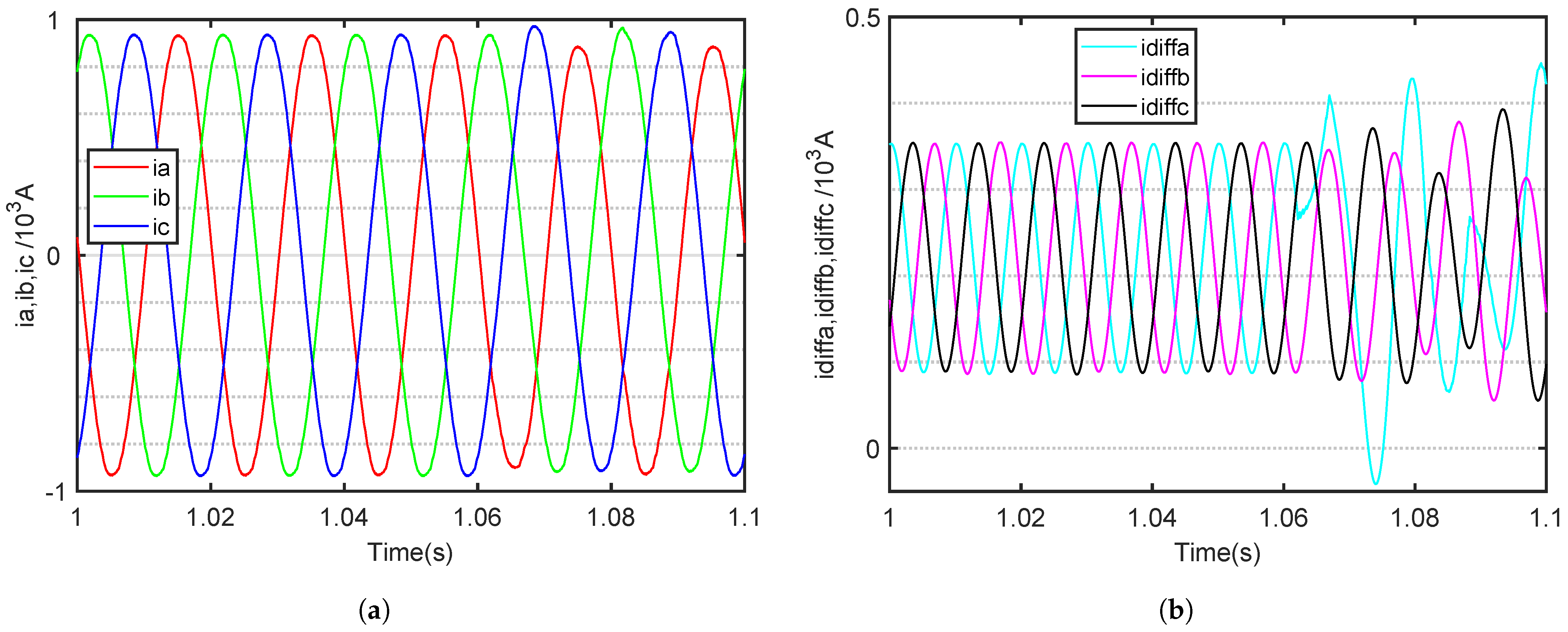
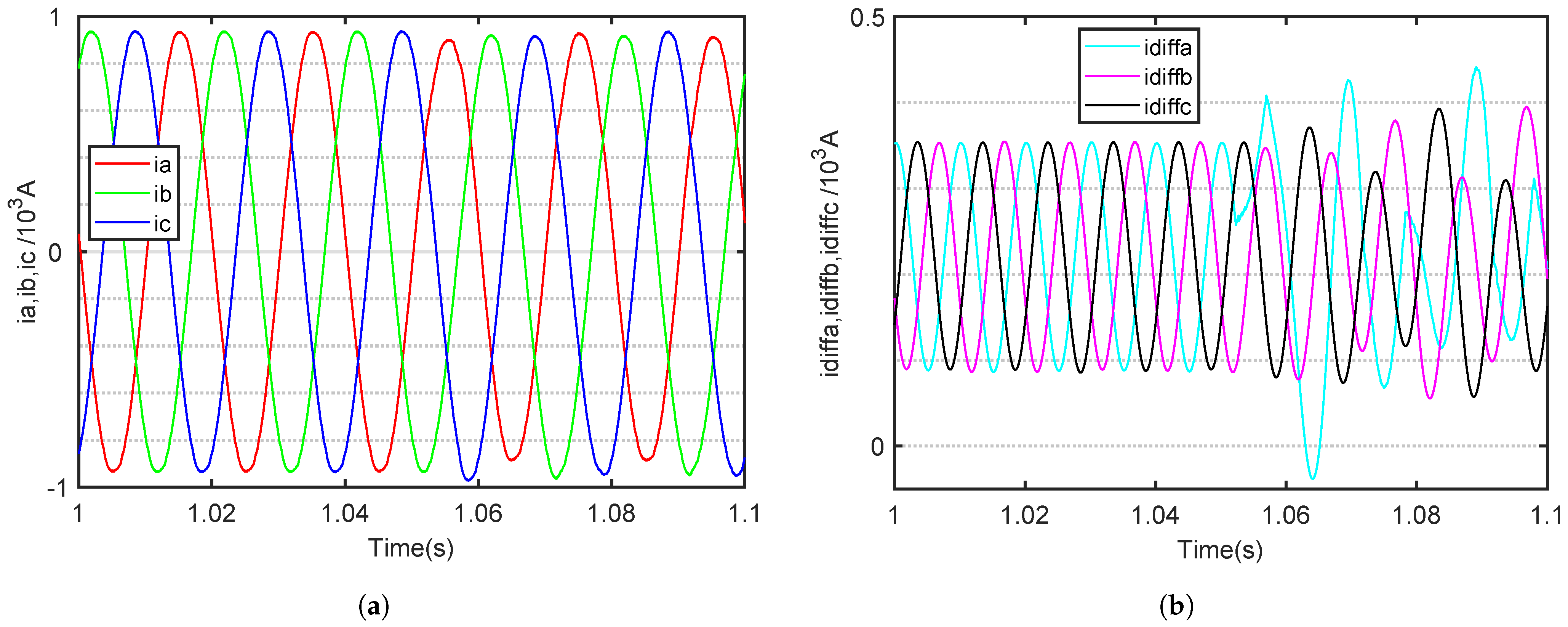
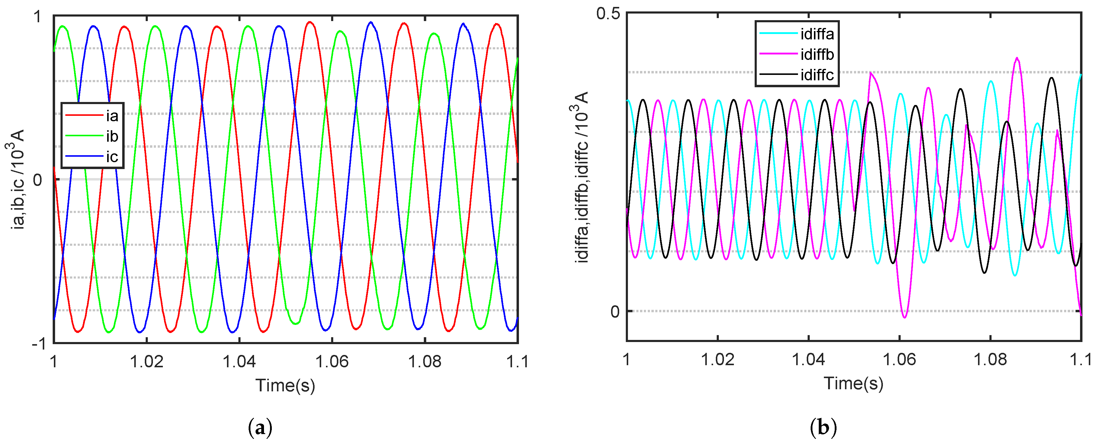
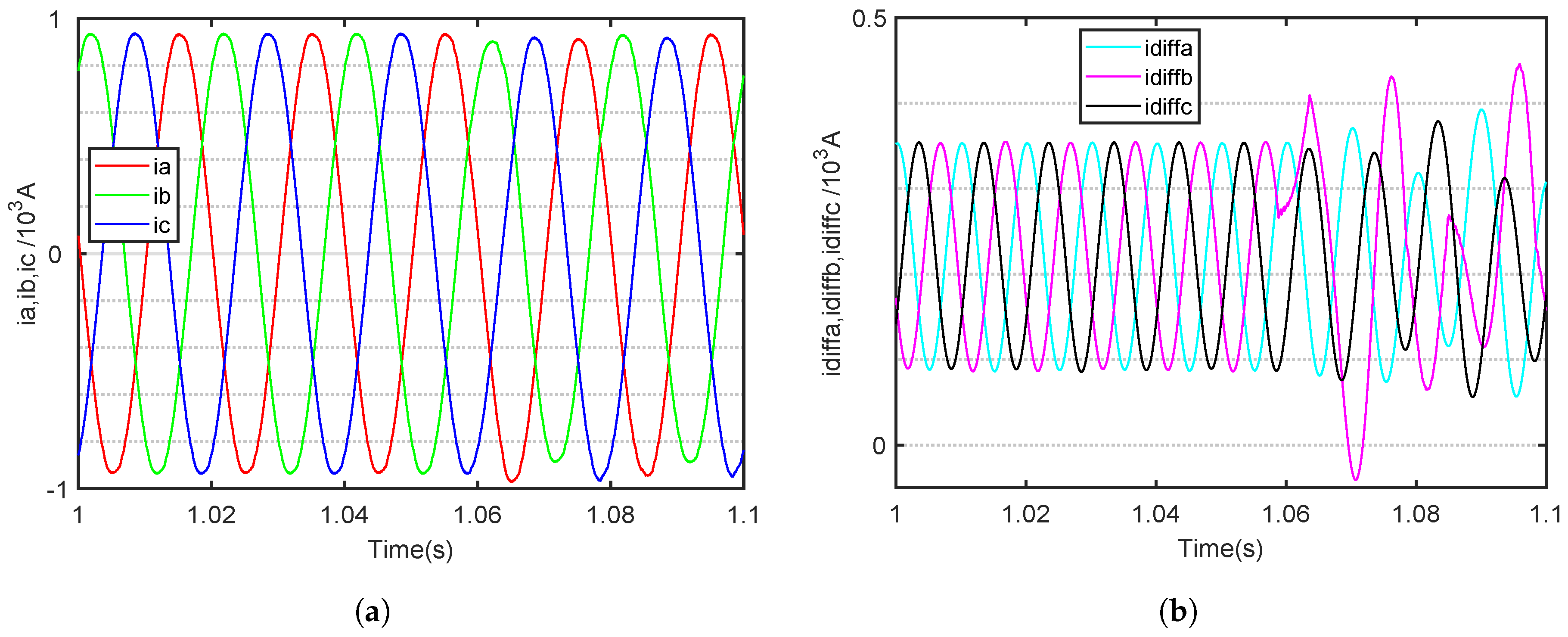
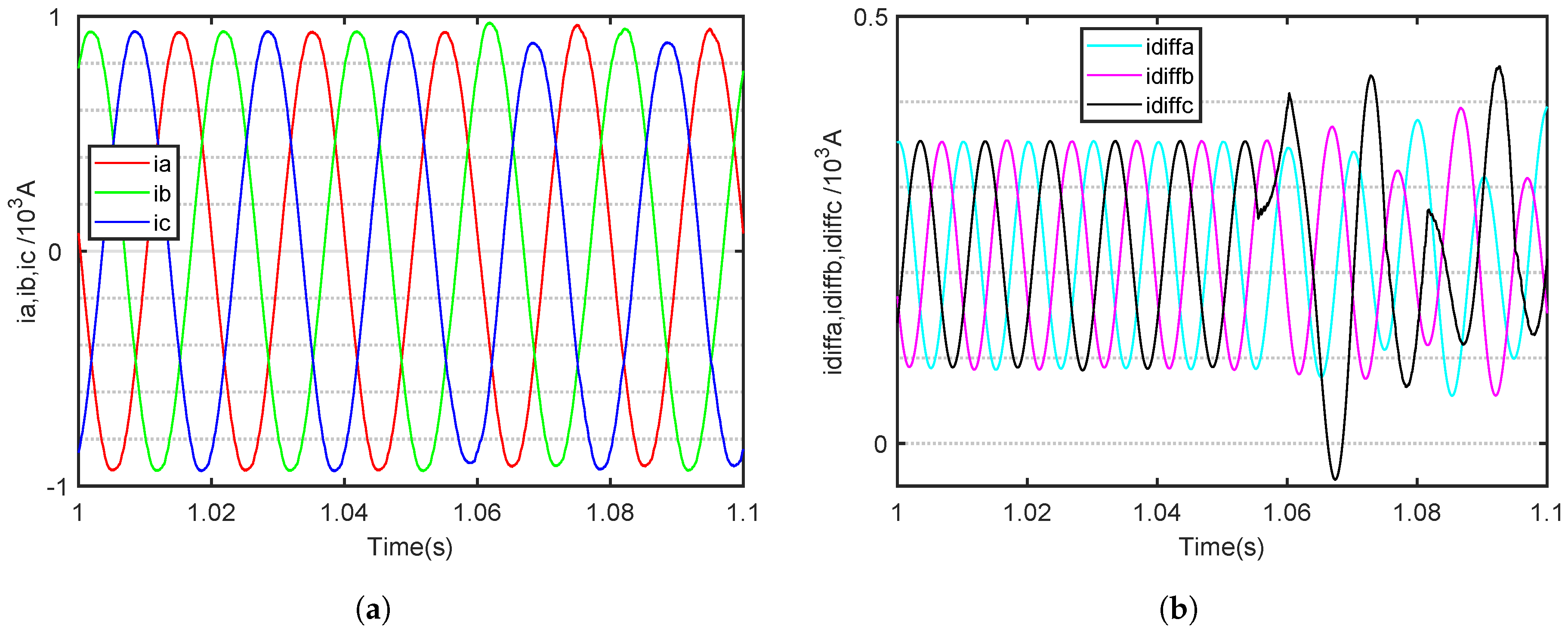
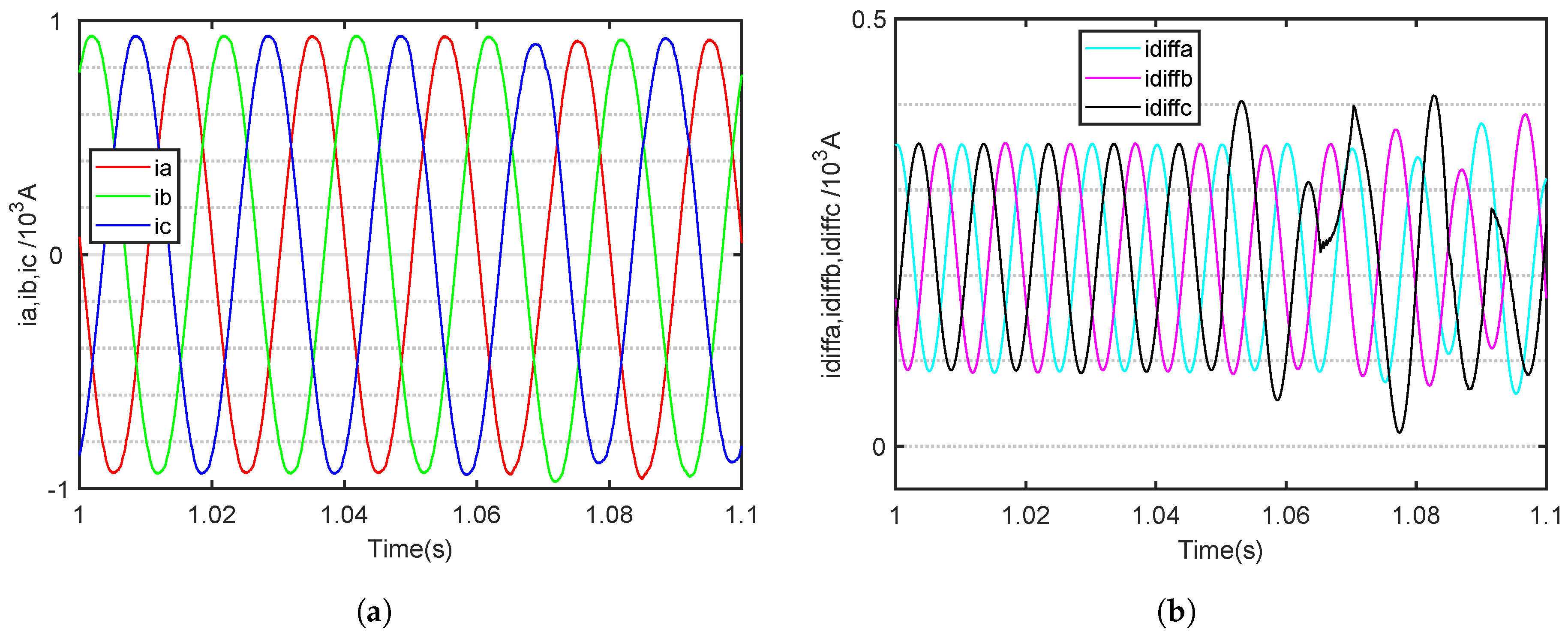
During normal operation, the three-phase output current of the MMC is symmetrical, with a phase difference of 120 degrees between the three phases. The internal circulating current of the three phases is also symmetrical. According to Equation (2), it can be concluded that the three-phase circulating current contains a DC bias component. The circulating current is a current with a relatively small amplitude and a large forward DC bias, which has twice the working frequency property. In addition, when an OC fault occurs in the SM of the MMC, the DC-side capacitor within the SM experiences abnormal charging and discharging. This irregularity leads to fluctuations in the capacitor voltage, which, in turn, alters the harmonic components of both the output current and the internal circulating current [5].

Taking the upper bridge arm of a phase A OC fault as an example, when an OC fault occurs in the SM, the AC output current of the faulted phase develops a negative DC offset. According to Kirchhoff’s current law, the sum of the three-phase AC currents entering the MMC at any moment must equal zero, resulting in the other two-phase AC currents developing a positive DC offset. The three-phase output cuurents are shown in Figure 5a, Figure 6a, Figure 7a, Figure 8a, Figure 9a and Figure 10a, respectively. From the output current waveform, it can be seen that the DC bias of the MMC output current is very small, and this bias characteristic is not obvious. Additionally, when an SM of a bridge arm experiences an OC fault, the amplitude of the output current of that phase will decrease, and the output current of the non-faulty phase will also decrease, but the magnitude of the decrease will not be as large as that of the faulty phase.

By contrast, the internal circulating current undergoes significant changes. It is evident that as the fault phase occurs, the circulating current of the fault phase increases, while the circulating current of the non-fault phase gradually decreases. The three-phase internal circuiting currents are shown in Figure 5b, Figure 6b, Figure 7b, Figure 8b, Figure 9b and Figure 10b, respectively.

Notably, when a fault occurs, the circulating current in the affected phase increases, while that in the unaffected phases gradually decreases. When an OC fault occurs in the SM of a bridge arm in a particular phase of the MMC, the asymmetrical operation of the bridge arm leads to significant fluctuations in the internal circulating current of the faulty phase. Meanwhile, the other two phases continue to operate normally, and all the increased components of the circulating current in the faulty phase’s bridge arm are directed towards the DC side. However, after an OC fault occurs in an MMC SM, it is important to note that the characteristics of the output time-domain current waveform become less apparent, especially as the number of MMC levels increases, causing these waveform features to become even less pronounced. 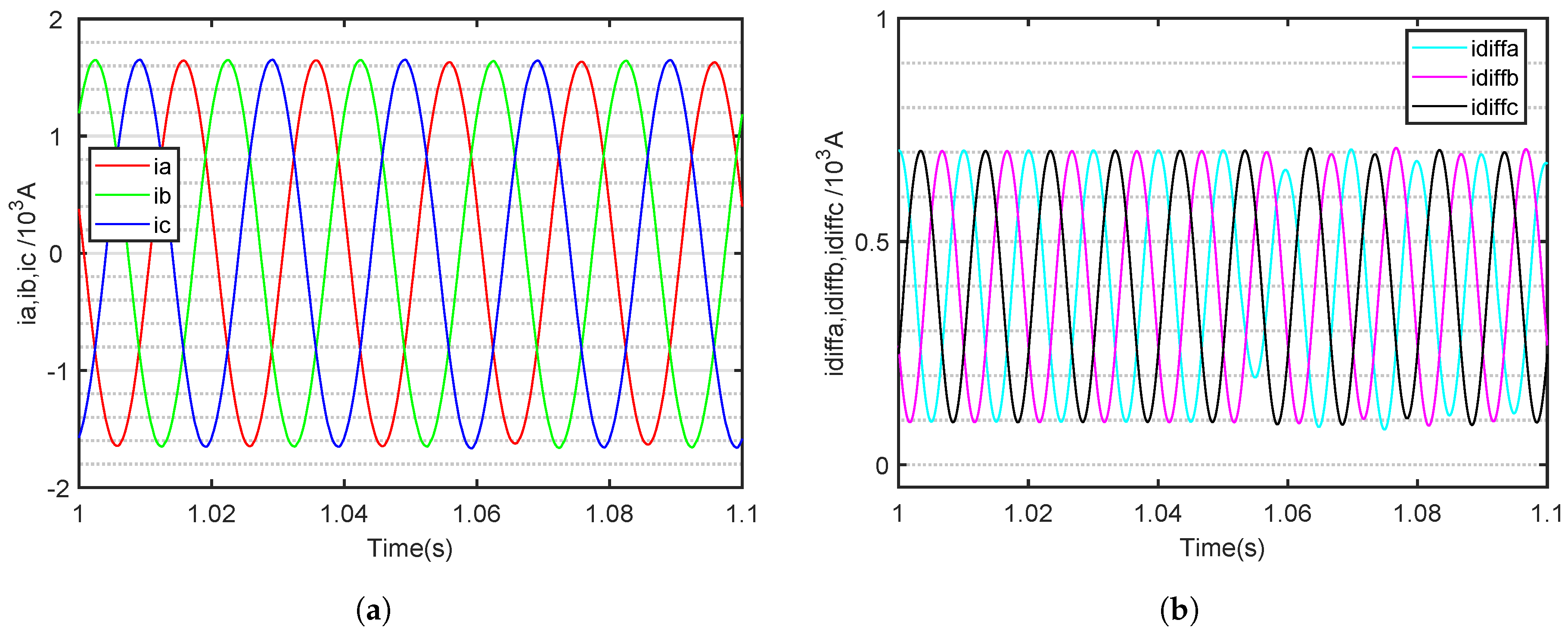Figure 11 shows the waveform of the OC fault point in the bridge arm SM of the 31-level MMC A-phase. Compared to the 11-level MMC, the current fault characteristics are less pronounced. When the MMC level is high, it means that the number of SMs connected in series increases, and the voltage contributed by each SM is only a small part of the total output voltage. The voltage waveform distortion caused by the failure of any single SM is masked by the many other SMs still working normally, so the variation in the output current waveform is not significant. Consequently, it is essential to explore a fault diagnosis method with advanced feature extraction capabilities for high-level MMC fault data.

4.1.2. Data Preprocessing and Dataset Segmentation

With the aim of preventing the model from overfitting and to improve the fitting effect for the proposed model, it is necessary to provide enough training samples. To this end, the dataset is expanded by resampling [18]. The resampling step size is set to 450, and each sample length is 2048. Finally, the training set, validation set, and test set data are split in a ratio of 8:1:1.

Taking into account that the values of the MMC AC output and circulating currents are quite different, if the initial features are not standardized, the accuracy may decrease, or the loss function may fail to converge during training. Accordingly, before the original data are fed into the model, the deviation standardization method is adopted to standardize all data. The formula is as follows:

$$\begin{array}{c}\hfill \tilde{\mathit{x}}={\displaystyle \frac{x-x_{min}}{x_{max}-x_{min}}}\end{array}$$

(15)

The number of the training sample set (NTRS) is 360, while the number of both the validation sample set (NVAS) and the testing sample set (NTES) is 40. The number of samples for each fault type is equal, as shown in

Table 3. Dataset segmentation and fault labels.

NTRS	NVAS	NTES	Fault Type	Fault Code	Fault Label
360	40	40	Normal	Nor	0
360	40	40	phase a upper	a1	1
360	40	40	phase a lower	a2	2
360	40	40	phase b upper	b1	3
360	40	40	phase b lower	b2	4
360	40	40	phase c upper	c1	5
360	40	40	phase c lower	c2	6

. To facilitate the calculation of the loss function, each sample is encoded using a 7-dimensional one-hot vector for the labels. In this encoding, each label is represented by a vector of all zeros, with a single element set to one at the index corresponding to the label.

4.2. Model Evaluation Metrics

This paper employs four common classification performance indicators to evaluate the performance of the fault diagnosis algorithm mentioned above, The four model evaluation metrics—Recall, Precision, F1, and Accuracy—are calculated utilizing the following equations:

$$\begin{array}{c}\hfill \mathit{Recall}={\displaystyle \frac{TP}{TP+FN}}\end{array}$$

(16)

$$\begin{array}{c}\hfill \mathit{Precision}={\displaystyle \frac{TP}{TP+FP}}\end{array}$$

(17)

$$\begin{array}{c}\hfill \mathit{F}\mathbf{1}={\displaystyle \frac{2Precision\times Recall}{Precision+Recall}}\end{array}$$

(18)

$$\begin{array}{c}\hfill \mathit{Accuracy}={\displaystyle \frac{TP+TN}{TP+TN+FP+FN}}\end{array}$$

(19)

where $TP$, $FP$, $TN$, and $FN$ denote true positive, false positive, true negative, and true negative, respectively. Samples are categorized into $TP$, $FP$, $TN$, and $FN$ based on the combination of actual categories and model predictions.

$$\begin{array}{c}\hfill \mathit{TPR}={\displaystyle \frac{TP}{TP+FN}}\end{array}$$

(20)

$$\begin{array}{c}\hfill \mathit{FPR}={\displaystyle \frac{FP}{FP+FN}}\end{array}$$

(21)

where $TPR$ and $FPR$ denote the true positive rate and false positive rate, respectively.

4.3. Model Parameter Settings

In the model training process, the adjustment of the hyperparameters, including the learning rate, batch size and activation function, plays an important role in the final training results. Among the adjustments, the setting of the learning rate parameters affects the convergence speed and performance of the model, which ultimately affects the model training. Therefore, it is very important to determine the range of the learning rate.

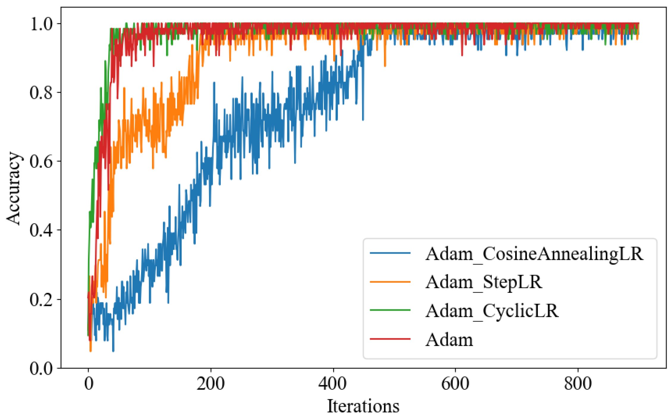
As shown in Figure 12, the accuracy of the model varies with the number of iterations under different combinations of the Adam optimizer and the learning rate schedulers. Among them, use of the Cyclic Learning Rate (CyclicLR) is a strategy that periodically adjusts the learning rate, such that it gradually increases from a small value to a larger value during the training process, and then gradually decreases back to a smaller value. StepLR gradually reduces the learning rate through multiplication factors after a predefined number of training steps. CosineAnnealingLR reduces the learning rate through a cosine function.

CyclicLR + Adam converges after about 50 iterations, and its convergence speed is slightly faster than the famous Adam optimizer. Adam + StepLR converges after about 200 iterations, and CosineAnnealingLR converges after about 500 iterations. Intuitively, as the number of training iterations increases, we should keep the learning rate decreasing in order to reach convergence at a certain point. However, contrary to intuition, using an LR that varies periodically within a given interval may be more useful. The reason is that the periodic high learning rate can make the model jump out of the local minima and saddle points encountered during the training process. Compared to local minima, saddle points hinder convergence more. If the saddle point happens to occur at a clever equilibrium point, a small learning rate usually cannot produce enough gradient changes to skip that point [35]. This is precisely where the periodic learning rate plays a role, as it can quickly bypass the saddle point. Another benefit is that the optimal LR will definitely fall between the minimum and maximum values. In other words, we used the best LR during the iteration process.

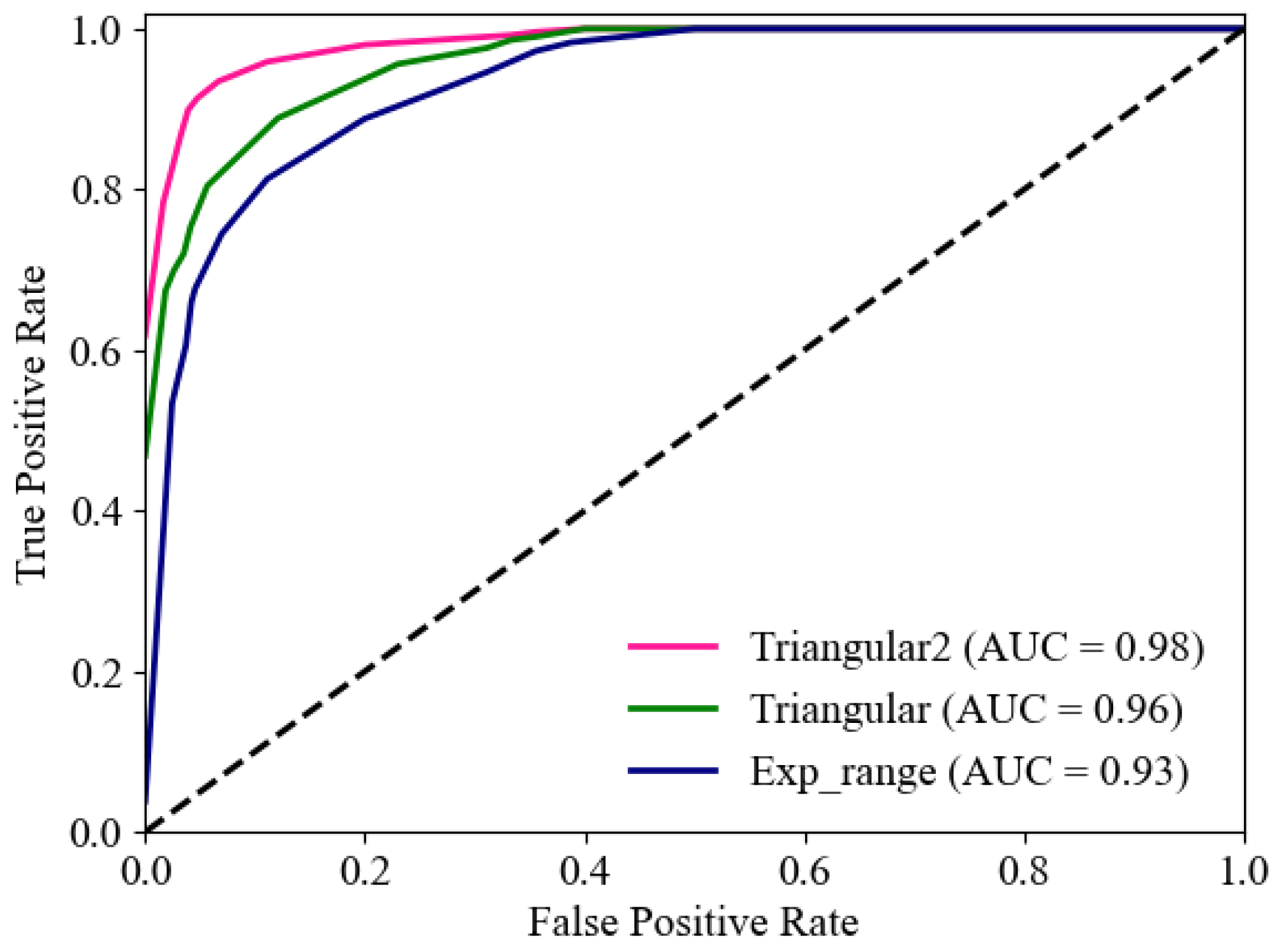
Therefore, this investigation adopts CyclicLR to effectively help the model jump out of local optima, avoid premature falling into local optima, and improve the model’s generalization ability. There are three different learning rate strategies in CyclicLR, including $triangular$, $triangular2$, and $exprange$. These three learning rates are entered into the model for training, and they are tested in the 31-level MMC dataset.

As can be seen from Figure 13, the three different learning rate strategies in CyclicLR match the model to differing degrees, and the ROC curve using the $triangular2$ learning rate is better than that of the other two learning rate strategies. Comparing the AUC under different learning rates, under the same network model, the AUC of the $triangular2$ learning rate strategy is the highest among the three different learning rate strategies. This shows that the $triangular2$ strategy has better convergence for network model training under CyclicLR.

4.4. Visualization and Analysis of the Model

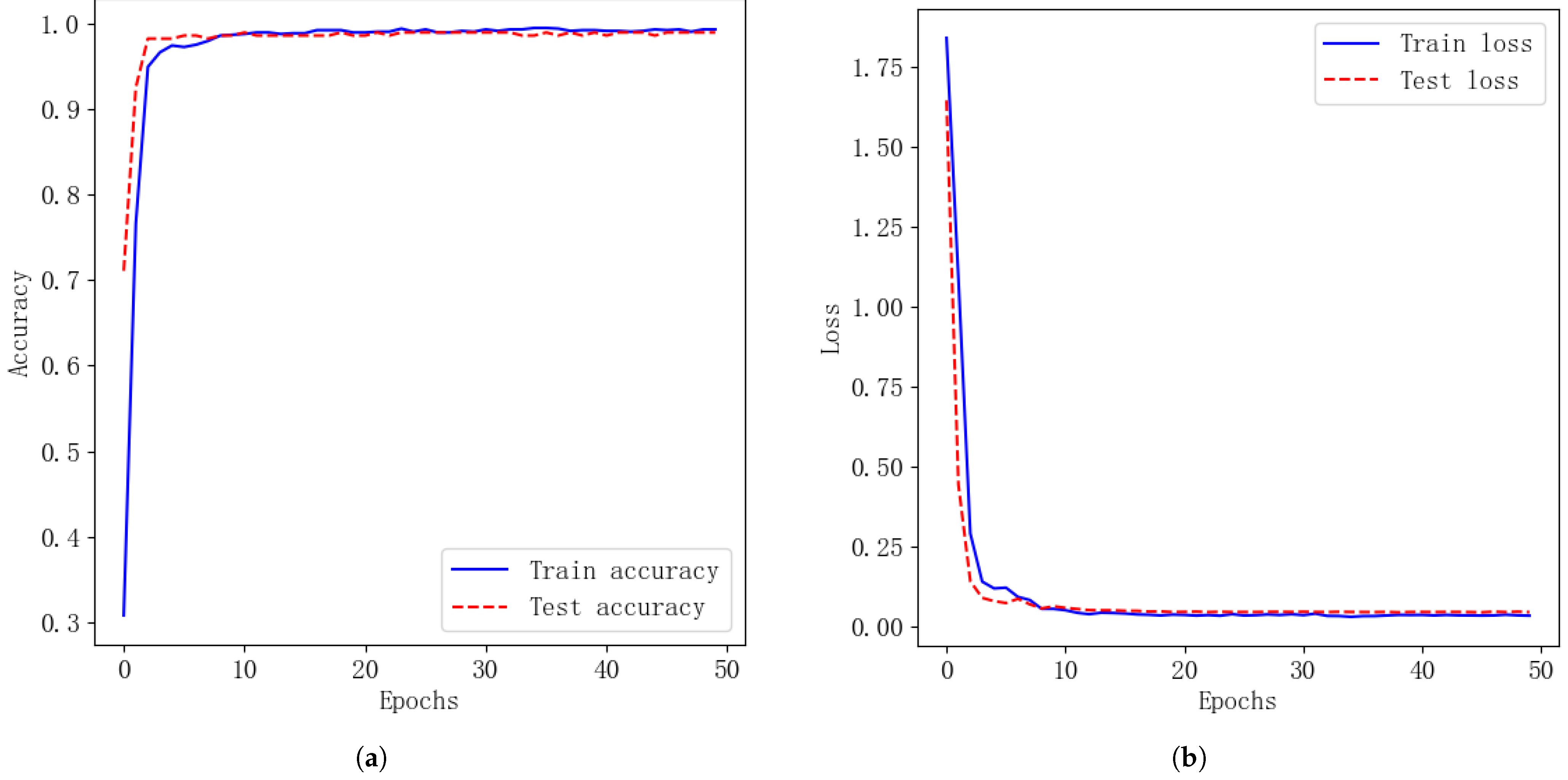
Figure 14 illustrates the convergence process of the MSAFN model as a function of the number of iterations, following multiple adjustments. It is clear that the loss function values for both the training and validation sets decrease as the number of iterations increases. When the number of epochs approaches 50, the loss function value and accuracy value of the model stabilize, which means that the loss and accuracy curve of the model has converged.

4.4.1. Visual Analysis of Training Process

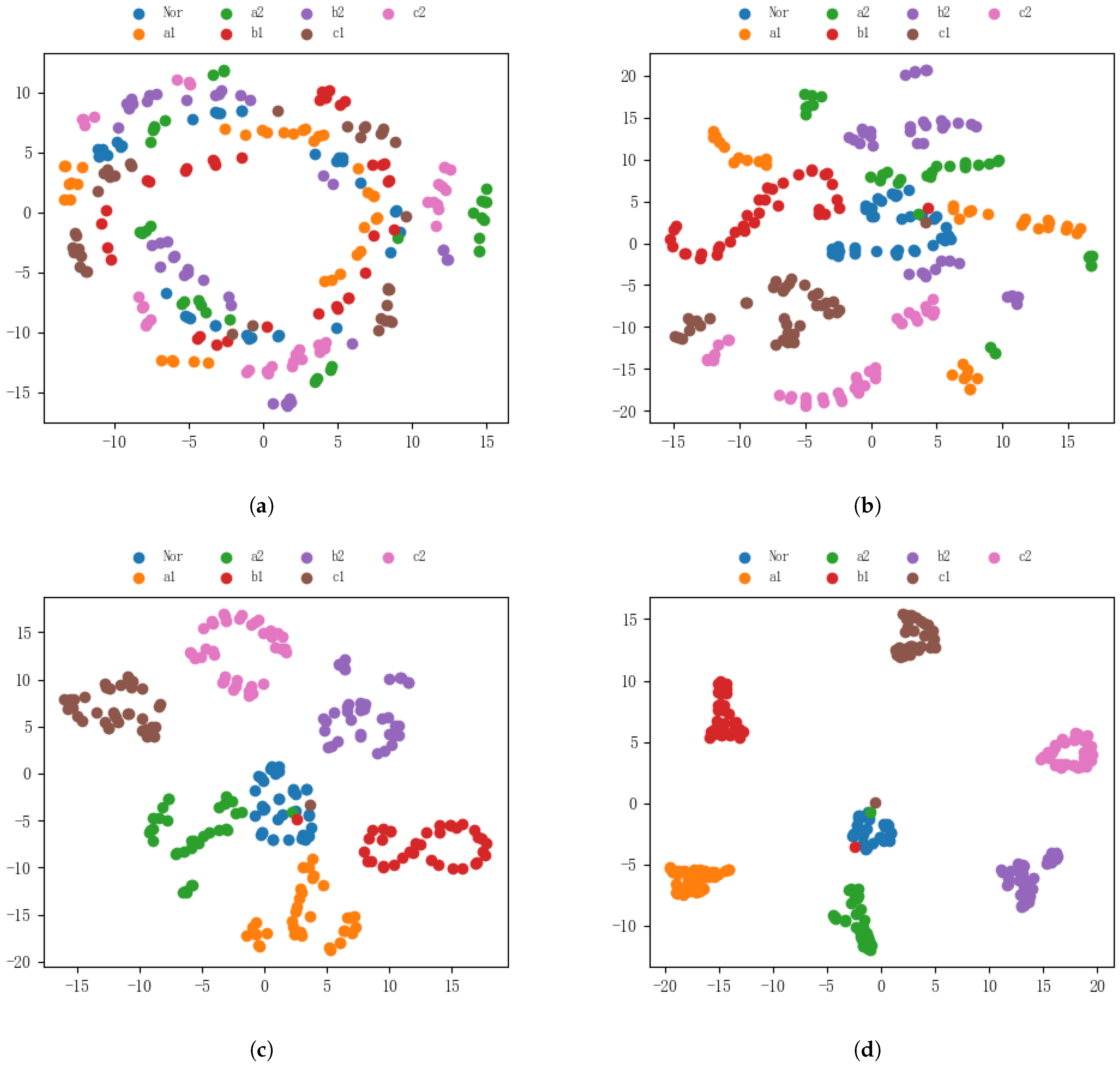
The t-SNE dimension reduction method can intuitively display the distribution of the data by linear projection of the data into two-dimensional space. This paper visualizes the training process of the model and observes the distribution of characteristics before and after the model training, as shown in Figure 15.

Figure 15a is the data distribution of the initial test set. It is obvious that the seven categories of data are completely inseparable at this time. In Figure 15b, after the data pass through the distribution of the attention mechanism layer of the first channel, the distance between the different classes is still small; there are obvious classifications, but the distance between classes is also insubstantial. Figure 15c shows the distribution of data through the fusion layer. It is found that with deepening of the network layer, the model gradually develops obvious classification boundaries for different types of data. Figure 15d is the distribution of data at the network output layer. It should be noted that the model can not only effectively classify different types of data, but also has a large distribution distance between categories and a small data distance within a category. In conclusion, the visualization results confirm that the MSAFN model enables effective diagnosis.

4.4.2. Analysis of Attention Effectiveness

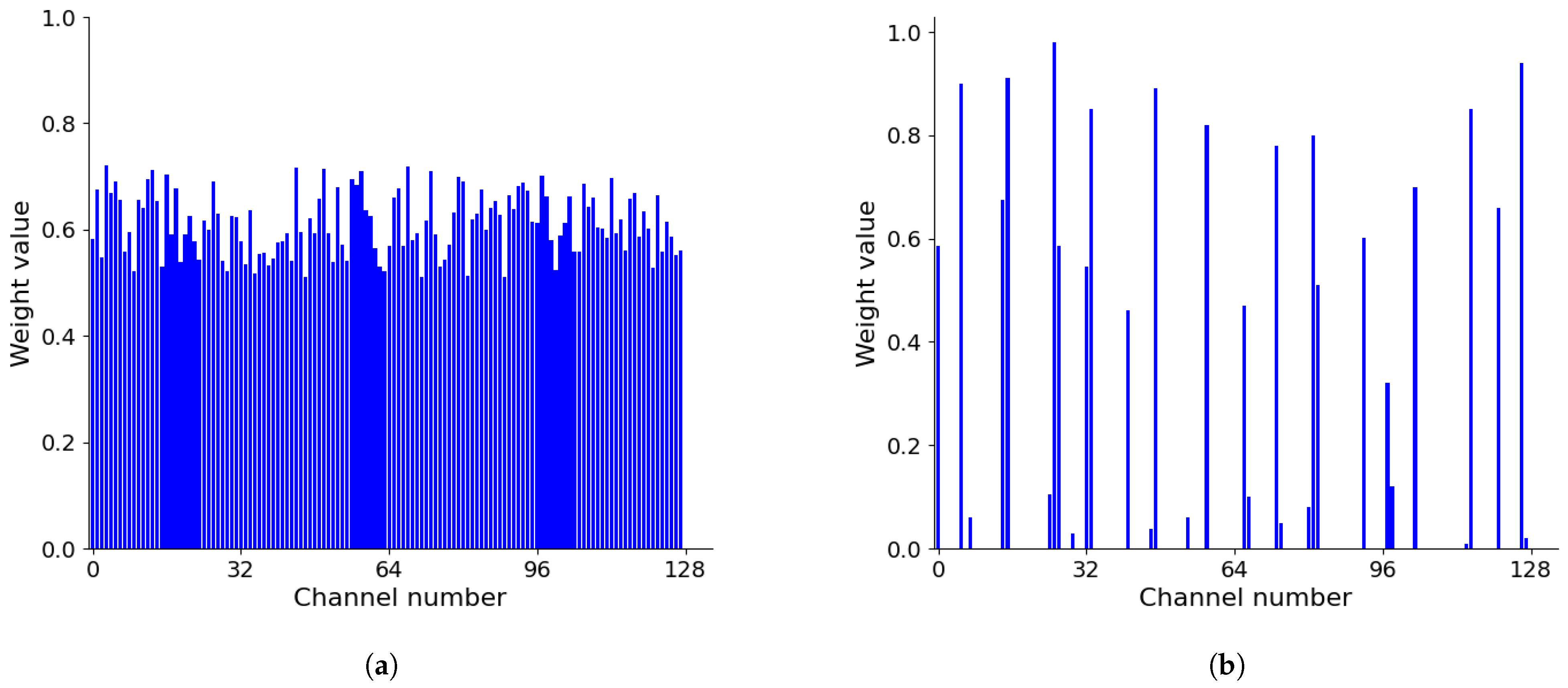
The changes in the weights of the proposed channel attention mechanism are analyzed during model training, which is employed to verify the effectiveness of the attention weight optimization process. Figure 16 shows the weight distribution of the three-phase output current in the second channel attention mechanism layer in convolution channel 1 when the model has just started six rounds of training and has finally converged. The number of channels in the second channel attention mechanism is 128.

As shown in Figure 16a, at the beginning of the training of the model, the attention weight values of each channel are basically close. In Figure 16b, when the model finally converges, the weights between the channels show a significant difference distribution, indicating that the channel attention mechanism has been parameter-modulated according to the criticality of the information in the channel. Consequently, the channel attention mechanism can effectively adjust the weight value through training so as to effectively mine the key fault features and suppress the features that are useless for fault diagnosis.

4.5. Anti-Noise Performance Analysis of the Model

To investigate the performance of the MSAFN model under noisy conditions, noise was added to the MMC current signal to simulate a real-world scenario. The added noise has varying signal-to-noise ratios (SNRs), with the calculation equation for the SNR as follows:

$$\begin{array}{c}\hfill \mathit{SNR}=10lo{g}_{10}\left({\displaystyle \frac{P_{signal}}{p_{noise}}}\right)\end{array}$$

(22)

where $P_{signal}$ represents the original signal power, and $P_{noise}$ represents the noise power.

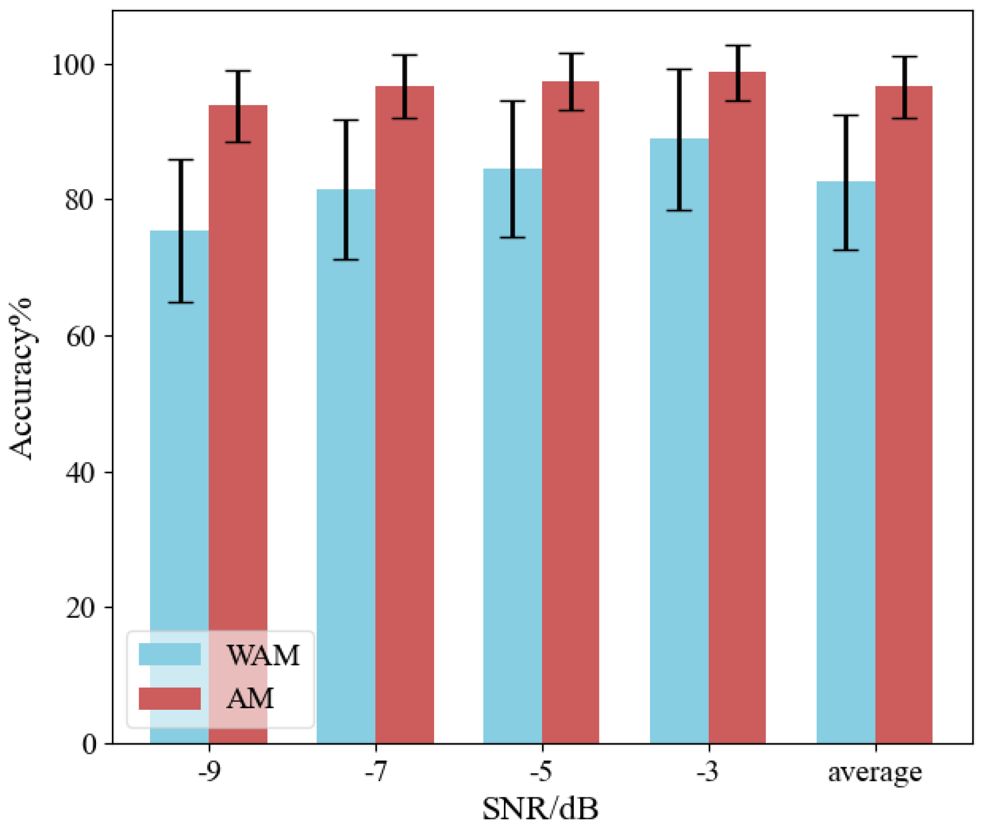
To validate the effectiveness of incorporating channel attention into the model, its impact on the model’s fault diagnosis accuracy was tested at SNRs of −3 dB, −5 dB, −7 dB, and −9 dB. The experiment was performed 10 times, and the results are shown in Figure 17. It is evident that models with attention mechanisms (AM) have better adaptive noise resistance compared to models without attention mechanisms (WAM). As the SNR decreases, the accuracy of model fault diagnosis will also decrease. MSAFN maintains good fault diagnosis accuracy during decrease in the SNR, with a minimum of $94.8\%$. The experimental results indicate that networks with added attention mechanisms can effectively suppress noise interference. The analysis results validated the performance of the MSAFN model and the effectiveness of the attention mechanism.

4.6. Comparison of Various Methods

4.6.1. Compare Methods of Baselines

For the purpose of verifing the effectiveness of the method proposed in this paper, we compare the MSAFN model with the most advanced fault diagnosis methods. The baseline methods for all comparisons are as follows:

1. MSCNN: MSCNN employs multiple convolutional paths, with the first layer consisting of three wide convolutional layers with kernel sizes of 100, 200, and 300, respectively. It then connects convolutional layers with kernel sizes of 8, 32, and 16 to extract features, demonstrating strong feature extraction ability [30].

2. WDCNN: The first layer of the WDCNN model is a wide convolution layer with a convolution core size of 64, and then four convolution layers with a convolution core size of 3 are connected to extract features [27].

3. MCNN: MCNN is a feature fusion layer that only uses the dense layer of the MSAFN model.

4. CNN-LSTM: CNN-LSTM introduces a long- and short-term memory network structure, which makes it easier to capture the features in the signal.

4.6.2. Experimental Results of Method Comparison

To compare the performance of the proposed model with other methods, ten tests were conducted in a noisy environment with an SNR of −9 dB. The performance test results of the four comparison models and the MSAFN model on the 31-level MMC dataset are presented in

Table 4. Performance measure of compared methods.

Model	Recall	Precision	F1	Accuracy
WDCNN	0.341	0.366	0.353	0.343
MCCNN	0.608	0.614	0.611	0.612
CNN-LSTM	0.607	0.635	0.621	0.624
MSCNN	0.822	0.818	0.820	0.816
MSAFN	0.932	0.951	0.941	0.948

. The experimental results indicate that the proposed MSAFN outperforms current state-of-the-art methods.

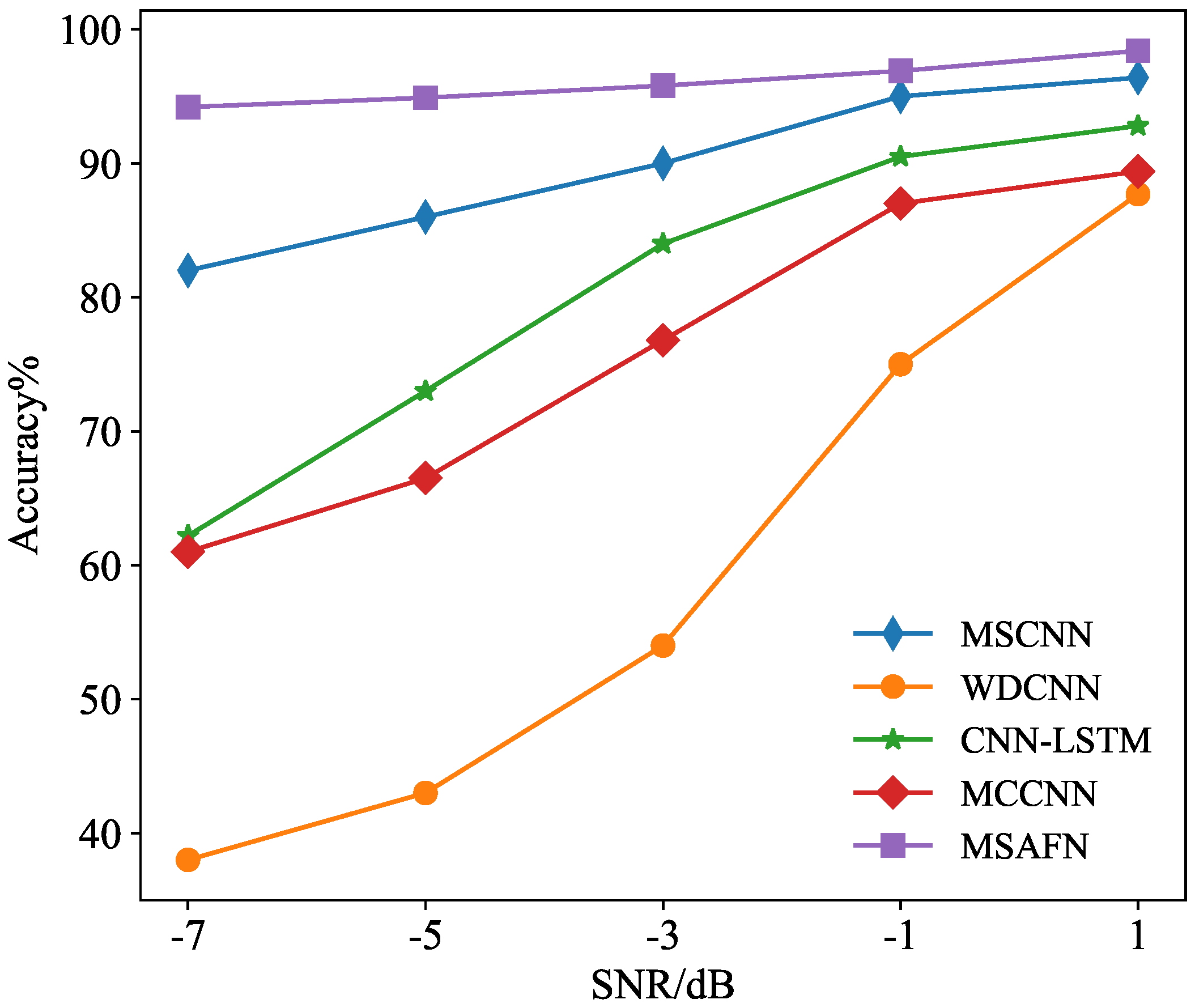
Method validation was conducted on current signals with an SNR ranging from −7 to 1 dB. The relationship between the recognition accuracy and the SNR for different methods is illustrated in Figure 18. As shown in the figure, as noise intensity increases, the accuracy of the four comparison methods decreases significantly. When the SNR is reduced to −7 dB, the accuracy of MSCNN, WDCNN, CNN-LSTM, and MCCNN is 81.6%, 34.3%, 62.4%, and 61.2%, respectively. Since MCNN has only a dense layer in the feature fusion layer, it easily overfits noise in a −7 dB environment, resulting in much lower diagnostic accuracy than MSAFN. The accuracy of MSAFN remains relatively stable across all noise levels, achieving 96.7% accuracy even at the lowest SNR of −7 dB, which is substantially higher than that of the other comparison methods. These findings suggest that the proposed MSAFN is more effective in handling noisy data scenarios.

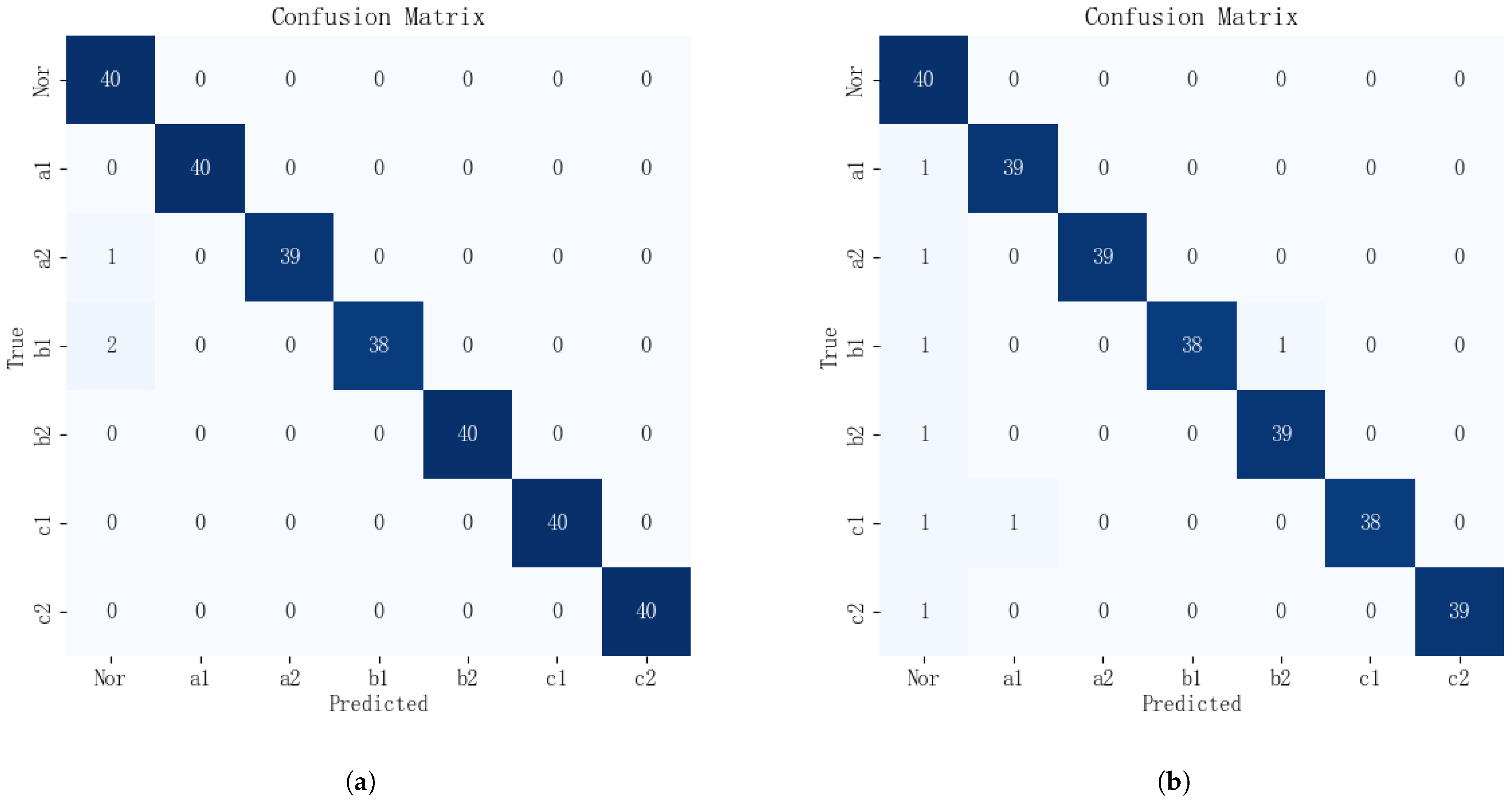
The fault diagnosis confusion matrices of the MSAFN on the 11-level and 31-level MMC test set data are shown in Figure 19, with 40 test samples for each fault category. The confusion matrix of the MSAFN method on the 11-level MMC dataset is shown in Figure 19a. It can be observed that one A-phase upper-bridge-arm sample was incorrectly classified as a normal sample, two B-phase upper-bridge-arm samples were wrongly classified as normal samples, and the remaining test samples were correctly identified. The confusion matrix of the MSAFN method on the 31-level MMC dataset is shown in Figure 19b. The figure shows that the classification accuracy is highest for samples with no faults and those considered normal. This is because, under normal conditions, the output and three-phase circulating currents of the MMC are symmetrical, and their time-domain characteristics are more pronounced compared to other fault types. In general, as the number of MMC levels increases, the current fault features of the MMC become less pronounced. However, the prediction accuracy for each sample type only experiences a slight decline. This indicates that the MSAFN model continues to deliver excellent diagnostic performance for high-level MMC fault detection.

5. Conclusions

This paper proposes a novel deep learning-based fault diagnosis framework, the Multiscale Adaptive Fusion Network (MSAFN), specifically designed to tackle the challenges of fault diagnosis in MMCs, especially in noisy environments. The framework first applies multiscale convolutions to extract critical fault features, followed by a channel attention mechanism to adaptively highlight key features. Next, adaptive 1D convolution is used for multiscale feature fusion, enhancing the model’s diagnostic performance in noisy environments. Experiments conducted on 11-level and 31-level MMC datasets demonstrate that MSAFN reliably identifies faults amidst noise. These results confirm that the proposed model effectively captures and fuses features across scales, enabling accurate fault identification even in complex environments. The broader significance of this work lies in its potential to enhance the reliability and operational stability of MMCs, which are critical in renewable energy integration and high-voltage applications. Beyond the immediate improvement in fault detection accuracy, this methodology advances the field by introducing a scalable diagnostic framework capable of adapting to various noise levels. This adaptability not only ensures robust performance across different operating conditions but also addresses one of the primary challenges in fault diagnosis—accurate detection amidst signal interference.

Furthermore, the proposed framework contributes to the ongoing development of intelligent diagnostic systems for power electronics by promoting generalization through cyclical learning rates and optimized convolutional architectures. Future research will focus on the following aspects: (1) Extending the model to imbalanced datasets and optimizing computational efficiency. (2) Building an MMC test prototype to extend fault diagnosis methods to industrial solutions, paving the way for real-time diagnostic applications in large-scale power systems.