Anti-Disturbance Target Tracking Control of Auxiliary Unmanned Ground Vehicles for Physical Education

Abstract

The auxiliary unmanned ground vehicle (AUGV) for physical education can significantly enhance the continuity and safety of training and competitions. However, obstacles and area boundary constraints present substantial challenges to the efficiency of the AUGV. This paper proposes an anti-disturbance target tracking control strategy for AUGV, enabling rapid tracking of out-of-bounds balls. In the guidance layer, we design safety constraints based on the exponentially stabilizing control Lyapunov function (ES-CLF) position constraint and control barrier function (CBF), and solve the expected convergence velocity guidance law through quadratic programming. Additionally, the expected motion direction of AUGV is determined using the expected combined velocity. In the control layer, we employ a nonlinear tracking differentiators (NLTD) to achieve finite-time estimation of the derivative of the guidance velocity signal, and observed the model parameter uncertainty and external environmental disturbances through a fixed time disturbance observer. Finally, a fixed-time control strategy is developed to achieve precise target tracking. Stability analysis and simulation results confirm the effectiveness of the proposed AUGV target tracking control strategy and the safety collision avoidance method.

1. Introduction

In recent years, integrating advanced unmanned technology with physical education has emerged as a key research focus. Rounds-based ball sports usually have characteristics such as relative enclosure, fixed boundaries, and clear field rules. When the rules are violated, auxiliary personnel will be equipped to pick up invalid balls and pass new balls, such as tennis and badminton. The advent of unmanned ground vehicles (UGV) as auxiliary tools in sports training and competition has shown promise in enhancing continuity, efficiency, and safety [1,2]. Among these, the physical education auxiliary unmanned ground vehicle (AUGV) as a significant stride towards automating and optimizing sports environments, which can perform tasks such as automatically picking up and removing boundary balls. However, the deployment of AUGVs in dynamic and constraint-laden environments introduces multifaceted challenges, primarily related to obstacle avoidance and autonomous navigation.

Common target tracking control strategies include PID control [3], sliding mode control [4], model predictive control (MPC) [5], and machine learning [6]. Specifically, PID controllers provide a basic framework for target tracking by continually adjusting the control inputs based on the difference between the desired and actual positions. However, PID controllers often struggle with complex dynamic environments due to their limited adaptability. The ability of MPC to handle multi-constraint environments makes it suitable for AUGV applications in sports fields. Nonetheless, the computational demands of real-time implementation remain a significant challenge. In addition, reinforcement learning provide the AUGV with the ability to learn from interactions with the environment, gradually improving their performance over time. However, the necessity for large datasets and substantial computational resources can be a limiting factor. Therefore, it is crucial to ensure precise tracking of task targets by the AUGV in high dynamic adversarial environments.

1.1. Related Work

Currently, the problem of dynamic target tracking is being explored and applied across various unmanned platforms in different dimensions. For instance, in UAV visual navigation, vision-based target tracking is utilized where speed and position information are acquired through visual means, thereby mitigating the impact of potential GPS failures. Besides, vision-based target tracking technology can also be applied to flight planning and obstacle avoidance [7]. In addition, a parallel approach guidance method is adopted in [8] to solve the problem of tracking a single moving target by a single unmanned surface vehicle (USV) during high-speed navigation. Reference [9] designed a neural-network-based target tracking controller for USV under complex marine environmental disturbances, which improved the robustness of the tracking controller. Du [10] proposed a finite-time convergent USV tracking controller that only requires relative distance and relative angle information for the target tracking problem with a partially known control input gain function. Bibuli [11] designed a parallel proximity guidance method based on sensors and communication systems, which achieved the tracking of high-speed linear motion targets by tracking virtual targets located near the target.

In contrast, the tracking accuracy of UGV for dynamic targets is constrained by environmental factors and both dynamic and static obstacles. Consequently, current research primarily focuses on methodologies such as MPC and behavior-based control, like finite state machines, to achieve safe and efficient target tracking. To accomplish precise trajectory tracking of moving targets by UGV, ref. [12] proposed an enhanced trajectory point tracking controller based on an improved MPC, capable of adapting to dynamic changes in vehicle speed and environment. In [13], the cost function incorporates reference path convergence and temporal convergence for the target tracking problem, establishing a nonlinear MPC framework. Ref. [14] introduced a robust tracking error-based MPC for controlling ground unmanned systems, with real-time evaluations of computational efficiency and tracking accuracy. However, the accuracy of MPC is limited by unmodeled dynamics such as tire slippage or nonlinear friction, which can directly affect control performance and is sensitive to environmental disturbances and dynamics. In comparison, nonlinear differential trackers, with their straightforward structure, naturally address common nonlinear characteristics in UGV systems, such as complex friction interactions between tires and the ground and dynamic modeling. They offer a reliable solution for precise and robust target tracking control in dynamic environments. References [15,16,17] integrated sliding mode control and finite-time control to design nonlinear differential trackers, achieving precise dynamic target tracking control for unmanned vehicles in the presence of unmodeled dynamics and external disturbances, thereby enhancing overall performance effectively.

In practical physical education competition environments, the AUGV encounters model variations caused by additional mass, unmodeled dynamics, and external environmental influences. To mitigate and eliminate the impact of uncertainties on motion control performance and to enhance the tracking accuracy, robustness, and stability of the AUGV, researchers have proposed various control strategies including sliding mode control [18,19], adaptive parameter control [20,21], neural network [22,23], fuzzy control [24,25], and active disturbance rejection control (ADRC) [26,27]. Among these, ADRC is distinguished by its ability to uniformly estimate both internal model disturbances and external environmental perturbations, and to compensate for them in the controller design. The extended state observer (ESO), as the keystone of ADRC, is lauded for its simplicity, ease of implementation, high precision, and robust anti-disturbance capability, which have been effectively validated in the tracking control of unmanned platforms. In [28,29], two ESOs were utilized to estimate disturbances in the forward velocity direction and yaw rate direction of the unmanned platform, and a cooperative path manipulation controller was designed based on these ESOs. In [30], the ESO was employed to estimate the unknown sideslip angle of the unmanned platform, and compensation for the sideslip angle was incorporated into the controller design, achieving coordinated control of multiple unmanned systems.

Based on the analysis of the aforementioned research, it is evident that the target tracking accuracy of the AUGV is constrained by internal and external disturbances, as well as dynamic and static obstacles, preventing the AUGV from fully achieving their expected performance. Therefore, proposing an autonomous collision avoidance and anti-disturbance dynamic target tracking control strategy is of paramount importance.

1.2. Main Contributions

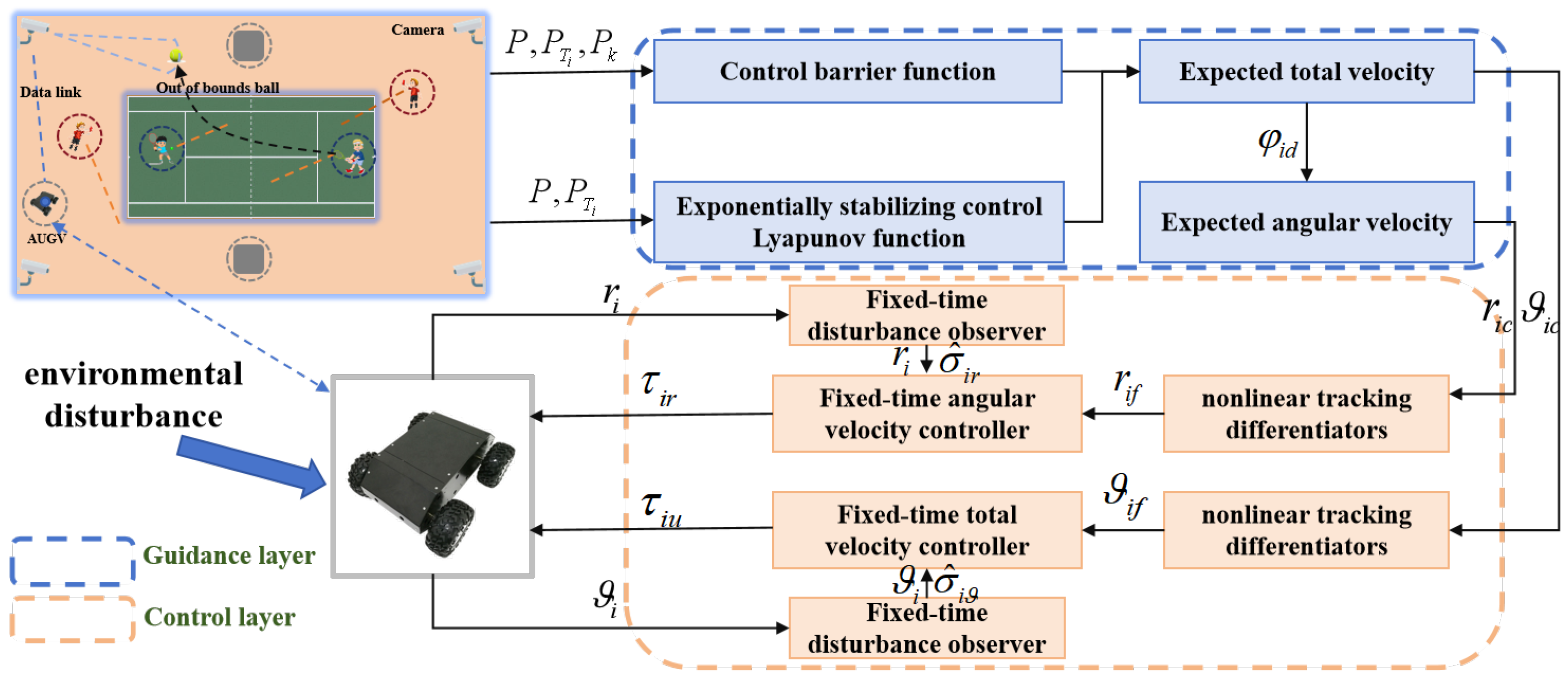
To enhance the performance of the physical education AUGV, this paper proposes an efficient dynamic target tracking control framework by integrating control barrier function (CBF), fixed-time control, and active disturbance rejection control. This framework enables rapid tracking of out-of-bounds balls under complex adversarial conditions. Specifically, precise guidance signals for dynamic targets are derived in the guidance layer, while accurate tracking of target speed and angle is achieved in the control layer. The main contributions are shown below.

(1).

In the guidance layer, we formulate a desired comprehensive velocity guidance law by leveraging the position constraint conditions derived from an exponentially stabilizing control Lyapunov function (ES-CLF) and integrating safety constraints based on CBF. This formulation is resolved through quadratic programming to ensure compliance with all specified constraints. The desired composite velocity is then used to determine the intended direction of the AUGV, and an angular velocity guidance law is designed accordingly.

(2).

In the control layer, we designed a nonlinear tracking differentiator to achieve finite-time estimation of the derivative of the guidance velocity signal, and a fixed-time disturbance observer (FTESO) is employed to monitor model parameter uncertainties and external environmental disturbances. Ultimately, we developed a fixed-time control law to enable precise target tracking.

(3).

We validated the proposed target tracking control strategy across several typical physical education application scenarios. Stability analysis and simulation results confirmed the effectiveness of the AUGV target tracking control strategy and the safety collision avoidance method.

The structure of this paper is as follows: Section 1 summarizes the research necessity and relevant studies. Section 2 provides a detailed description of the AUGV dynamic target tracking problem. Section 3 elaborates on the core algorithms presented in this paper. Section 4 presents the experimental validation and analysis. Section 5 concludes the paper.

2. AUGV Model and Problem Formulation

We define a general physical education competition venue model as shown in Figure 1a, which includes an effective rectangle adversarial area and an auxiliary rectangle area. The AUGV needs to quickly track and pick up out of bounds balls within the auxiliary area, while avoiding collisions with moving referees. This section provides a detailed description of the mathematical model of AUGV and the problem we solved.

2.1. AUGV Model

In order to fit the task scenario, we consider the underactuated AUGV driving on good road conditions with low speed. To ensure the effectiveness of the target tracking control algorithm and reduce the complexity of theoretical derivation, we adopt a particle model that meets the basic task requirements to replace the complex AUGV mathematical model. As shown in Figure 1b, the coordinate system $O_{\mathrm{E}}{X}_{\mathrm{E}}{Y}_{\mathrm{E}}$ is the earth coordinate system tangent to the surface of earth, and the coordinate system $O_{\mathrm{B}}{X}_{\mathrm{B}}{Y}_{\mathrm{B}}$ is the fixed-body coordinate system. Moreover, $O_{\mathrm{B}}$ is the center of AUGV, $O_{\mathrm{B}}{X}_{\mathrm{B}}$ is towards the front of the AUGV and is parallel to the ground, and $O_{\mathrm{B}}{Y}_{\mathrm{B}}$ is perpendicular to $O_{\mathrm{B}}{X}_{\mathrm{B}}$ and parallel to the ground. Then, the kinematic and dynamic models of the AUGV containing unmodeled dynamics and unknown disturbances can be obtained as [31]:

$$\begin{array}{c}\begin{array}{c}\begin{array}{c}\dot{\mathit{\eta }}=\mathit{R}\left(\mathit{\phi }\right)\mathit{v}\\ \mathit{M}\dot{\mathit{v}}=-\mathit{G}\left(\mathit{v}\right)\mathit{v}+\mathit{\tau }+{\mathit{\tau }}_{\mathit{d}}\left(t\right)\end{array}\hfill \end{array}\end{array}$$

(1)

where $\mathit{\eta }={[x,y,\phi ]}^{\mathrm{T}}\in {\mathrm{R}}^3$ represents the position and heading angle of AUGV in the earth coordinate system, $\mathit{v}={[u,\upsilon ,r]}^{\mathrm{T}}\in {\mathrm{R}}^3$ represent the forward velocity, lateral velocity, and angular velocity of AUGV in the fixed-body coordinate system, respectively, $\mathit{\tau }={\left[{\tau }_u,0,{\tau }_r\right]}^{\mathrm{T}}\in {\mathrm{R}}^3$ represents the control input vector of the AUGV, ${\mathit{\tau }}_{\mathit{d}}={\left[{\tau }_{wu},{\tau }_{w\upsilon },{\tau }_{wr}\right]}^{\mathrm{T}}\in {\mathrm{R}}^3$ represents external environmental disturbance, and $\mathit{R}\left(\mathit{\phi }\right)$ represents the rotation matrix from the fixed-body coordinate system to the earth coordinate system, expressed as follows:

$$\begin{array}{c}\begin{array}{c}\mathit{R}\left(\mathit{\phi }\right)=\left[\begin{array}{ccc}cos\phi & -sin\phi & 0\\ sin\phi & cos\phi & 0\\ 0& 0& 1\end{array}\right]\hfill \end{array}\end{array}$$

(2)

In the dynamic model, $\mathit{M}=\mathrm{diag}\{m_u,m_v,m_r\}\in {\mathrm{R}}^{3\times 3}$ represents the mass matrix and $\mathit{G}\left(\mathit{v}\right)=\mathit{C}\left(\mathit{v}\right)+\mathit{D}\left(\mathit{v}\right)$ represents the Coriolis centripetal force matrix and damping matrix, expressed as follows:

$$\begin{array}{c}\begin{array}{c}\mathit{C}\left(\mathit{v}\right)=\left[\begin{array}{ccc}0& 0& c_{13}\\ 0& 0& c_{23}\\ c_{31}& c_{32}& 0\end{array}\right]\mathit{D}\left(\mathit{v}\right)=\left[\begin{array}{ccc}{d}_{11}& 0& 0\\ 0& d_{22}& d_{23}\\ 0& d_{32}& d_{33}\end{array}\right]\hfill \end{array}\end{array}$$

(3)

Remark 1. 

We use the particle model instead of the complex UAGV mathematical model to simplify problem analysis while ensuring the wide applicability of the proposed target tracking strategy.

2.2. Problem Formulation

The triggering condition for the physical education AUGV to perform target tracking tasks is that the ball is hit out of the adversarial area. We define the position of out-of-bounds balls as ${\mathit{P}}_{T_i}$, which is monitored by the position system and transmitted to the AUGV. After receiving the task instruction, we define the distance $e_i$ and angle ${\beta }_i$ between the AUGV and the target $T_i$ as follows:

$$\begin{array}{c}{e}_i=\sqrt{{\left(p_{T_{i}x}-x\right)}^2+{\left(p_{T_{i}y}-y\right)}^2}\\ {\beta }_i=\mathrm{arc}tan2\left({\displaystyle \frac{p_{T_{i}y}-y}{p_{T_{i}x}-x}}\right)\end{array}$$

(4)

where $\mathit{P}={[x,y]}^{\mathrm{T}}$ and ${\mathit{P}}_{T_i}={[p_{T_{i}x},p_{T_{i}y}]}^{\mathrm{T}}$ are the position vectors of the AUGV and task point, respectively.

The tracking error between the AUGV and the task point is as follows:

$$\begin{array}{c}{e}_{ip}=e_i-{\lambda }_i\\ e_{i\beta }={\beta }_i-{\phi }_i\end{array}$$

(5)

where ${\lambda }_i\in {\mathrm{R}}^{+}$ is a small constant.

In the ideal environment, the purpose of this paper is to propose a target tracking control strategy for the physical education AUGV to achieve the following objectives. Position tracking: drive the AUGV to approach the target point ${\mathit{P}}_{T_i}$ and make the position error $e_{ip}$ satisfies $\underset{t\to \infty }{lim}{e}_{ip}=0$. Heading tracking: drive the heading error $e_{i\beta }$ between the actual heading and the expected heading of the AUGV satisfies $\underset{t\to \infty }{lim}{e}_{i\beta }=0$.

In the environment with multiple dynamic and static obstacles, we assume that there are M dynamic and static obstacles within the competition area, the position of the obstacle k is ${\mathit{P}}_k={[x_k,y_k]}^{\mathrm{T}}\in {\mathrm{R}}^2$, and the moving speed of the obstacle k in the earth coordinate system is ${\mathit{q}}_k\in {\mathrm{R}}^2$ with a radius of $h_k\in {\mathrm{R}}^{+},k=1,\cdots ,M$. The purpose of this paper is to design an anti-disturbance target tracking and collision avoidance control strategies to achieve the following objectives:

(1).

Geometric objective: Drive the AUGV to track task target, as shown below:

$$\begin{array}{c}\underset{t\to \infty }{lim}∥\mathit{P}-{\mathit{P}}_{T_i}∥\le {\epsilon }_{i1}\end{array}$$

(6)

where ${\epsilon }_{i1}\in {\mathrm{R}}^{+}$ is a small positive number.

(2).

Collision avoidance target: Ensure that the distance between the AUGV and the obstacle satisfies:

$$\begin{array}{c}∥\mathit{P}-{\mathit{P}}_k∥>D+h_k\end{array}$$

(7)

where ${\mathit{P}}_k\in {\mathrm{R}}^2$ represents the position vector of obstacle in the earth coordinate system and $D_k\in {\mathrm{R}}^{+}$ indicates the maximum obstacle avoidance distance of the AUGV.

3. Design of the Trajectory Tracking Control Strategy

The purpose of this section is to design an anti-disturbance target tracking controller for the AUGV, aimed at achieving control objectives (6) and (7). Specifically, the guidance layer is tasked with designing the guidance laws for the desired combined velocity and angular velocity of the AUGV. This is achieved by employing a nonlinear differentiator to enable finite-time estimation of the derivatives of the guidance signals. At the control layer, a fixed-time disturdance observer (FTDO) is designed to estimate the total system disturbance. Subsequently, a fixed-time control strategy is crafted to accurately track the desired guidance velocity. The specific control framework is illustrated in Figure 2, where the indoor positioning system obtains the position of the AUGV, the position of dynamic targets, and the position information of obstacles to CBF and exponential stabilizing control Lyapunov function to get the expected total velocity and expected angular velocity. Then, we process the obtained velocity guidance signal and angular velocity guidance signal separately through two nonlinear tracking differentiators, and the processed information is transmitted to two fixed-time controllers to obtain the final control input of the AUGV.

Design of Guidance Layer

To simplify the analysis, we transform the kinematic and dynamic models of the AUGV as follows:

$$\begin{array}{c}\begin{array}{c}\dot{x}=Vcos\phi \\ \dot{y}=Vsin\phi \\ \dot{\phi }=r+\dot{\beta }\end{array}\end{array}$$

(8)

and

$$\begin{array}{c}\begin{array}{c}{m}_u\dot{V}=f_u(·)+{\tau }_u+{\tau }_{wu}\left(t\right)+2m_u\dot{V}{sin}^2\left({\displaystyle \frac{\beta }{2}}\right)+m_{u}Vsin\left(\beta \right){\beta }_d\\ m_r\dot{r}=f_r(·)+{\tau }_r+{\tau }_{wr}\left(t\right)\end{array}\end{array}$$

(9)

where $V=\sqrt{u^2+{\upsilon }^2}$ is the total velocity of the UAGV, $\phi =\psi +\beta$, and $\beta =arctan2(\upsilon ,u)$ represents the sideslip angle generated by the speed v.

4. Design of Target Tracking Controller

The purpose of this section is to achieve the control objectives (6) and (7). Specifically, the controller design consists of a guidance layer and a control layer. In the guidance layer, desired composite velocity and angular velocity guidance laws are developed. In the control layer, a FTESO is designed to estimate total system disturbances, and a fixed-time control law is formulated to track the desired guidance velocities. A nonlinear differentiator is also designed to achieve finite-time estimation of the derivatives of the guidance signals.

4.1. Design of Guidance Layer

In this subsection, we design desired composite velocity and angular velocity guidance laws to achieve dynamic target tracking and collision avoidance for the AUGV. For the desired composite velocity guidance law, we use the following three steps.

(1).

Position constraint design based on ES-CLF

To ensure that the AUGV can track the optimal target point and minimize the position cost function, a Lyapunov function (ES-CLF) can be constructed as follows:

$$\begin{array}{c}{V}_{i1}={\displaystyle \frac{1}{2}}{∥\mathit{P}-{\mathit{P}}_{T_i}∥}^2\end{array}$$

(10)

and the definition of a superzero level set is:

$$\begin{array}{c}{S}_{T_i}=\left\{\mathit{P}\left|V_{i1}\le 0\right.\right\}\end{array}$$

(11)

We define the tracking error vector between the AUGV and its target point ${\mathit{P}}_{T_i}$ as ${\mathit{P}}_{ie}=\mathit{P}-{\mathit{P}}_{T_i}$. By differentiating (10), we obtain:

$$\begin{array}{c}{\dot{V}}_{i1}={{\mathit{P}}_{ie}}^{\mathrm{T}}({\mathit{q}}_i-\dot{{\mathit{P}}_{T_i}})\end{array}$$

(12)

Definition 1 

([32]). Consider the following form of nonlinear affine control system:

$$\begin{array}{c}\dot{\mathit{x}}=\mathit{f}\left(\mathit{x}\right)+\mathit{g}\left(\mathit{x}\right)\mathit{u}\end{array}$$

(13)

where $\mathit{x}\in {\mathrm{R}}^n$ represents the state variables of the system, and $\mathit{u}\in {\mathrm{R}}^m$ represents the control inputs of the system. $\mathit{f}\left(\mathit{x}\right)\in {\mathrm{R}}^n$ and $\mathit{g}\left(\mathit{x}\right)\in {\mathrm{R}}^{n\times m}$ represent local Lipschitz continuous functions.

We define a continuously differentiable function $V:{\mathrm{R}}^n\to \mathrm{R}$, and if there are constants $c_1,c_2,c_3\in {\mathrm{R}}^{+}$ that (14) holds for any $x\in {\mathrm{R}}^n$, then the function V is an exponentially stable control Lyapunov function (ES-CLF):

$$\begin{array}{c}\begin{array}{c}{c}_1{∥\mathit{x}∥}^2\le V\left(\mathit{x}\right)\le c_2{∥\mathit{x}∥}^2\hfill \\ \underset{u\in U}{inf}\left[L_{f}V\left(\mathit{x}\right)+L_{g}V\left(\mathit{x}\right)\mathit{u}+c_{3}V\left(\mathit{x}\right)\right]\le 0\hfill \end{array}\end{array}$$

(14)

where $L_{f}V\left(\mathit{x}\right)$ and $L_{g}V\left(\mathit{x}\right)$ represent the Lie derivative of $V\left(\mathit{x}\right)$.

For a given ES-CLF, define the following set of control input constraints:

$$\begin{array}{c}{K}_{\mathrm{clf}}\left(\mathit{x}\right)=\left\{\mathit{u}\in U:L_{f}V\left(\mathit{x}\right)+L_{g}V\left(\mathit{x}\right)\mathit{u}+c_{3}V\left(\mathit{x}\right)\le 0\right\}\end{array}$$

(15)

If any local Lipschitz continuous control input is $\mathit{u}\in K_{\mathrm{clf}}\left(\mathit{x}\right)$, then the solution of the system (13) satisfies:

$$\begin{array}{c}∥\mathit{x}\left(t\right)∥\le \sqrt{{\displaystyle \frac{c_2}{c_1}}}{e}^{-{\displaystyle \frac{c_3}{2}}t}∥\mathit{x}\left(0\right)∥\end{array}$$

(16)

Then, according to Definition 1, the constraint satisfying ES-CLF is:

$$\begin{array}{c}{{\mathit{P}}_{ie}}^{\mathrm{T}}({\mathit{q}}_i-\dot{{\mathit{P}}_{T_i}})+c_1{V}_{i1}\le 0\end{array}$$

(17)

where $c_1>0$ is a small constant.

(2).

Security constraint design based on CBF

To ensure the motion safety of the AUGV during dynamic target tracking and prevent collision with dynamic and static obstacles, i.e., control objective (7), the following continuous differentiable function $h_i\left(\mathit{P}\right)$ is designed:

$$\begin{array}{c}{h}_i\left(p_i\right)={∥\mathit{P}-{\mathit{P}}_{T_i}∥}^2-{(D_i+h_i)}^2\end{array}$$

(18)

where the security set ${\mathcal{C}}_i$ can be represented as:

$$\begin{array}{c}{\mathcal{C}}_i=\left\{\mathit{P}\left|h_i\left(\mathit{P}\right)\right.\ge 0\right\}\end{array}$$

(19)

Definition 2 

([33]). If $h\left(\mathit{x}\right):{\mathrm{R}}^n\to \mathrm{R}$ is a continuously differentiable function, then the safety set $\mathcal{C}\subset {\mathrm{R}}^n$ satisfies the following condition:

$$\begin{array}{c}\begin{array}{c}\mathcal{C}=\left\{\mathit{x}\in {\mathrm{R}}^n:h\left(\mathit{x}\right)\ge 0\right\}\\ \partial \mathcal{C}=\left\{\mathit{x}\in {\mathrm{R}}^n:h\left(\mathit{x}\right)=0\right\}\\ \mathrm{Int}(\mathcal{C})=\left\{\mathit{x}\in {\mathrm{R}}^n:h\left(\mathit{x}\right)>0\right\}\end{array}\end{array}$$

(20)

If there are $\mathit{x}\left(0\right)\in \mathcal{C}$, $\mathit{x}\left(t\right)\in \mathcal{C}$ for any initial value $\mathit{x}\left(t_0\right)\in \mathcal{C}$, then the set $\mathcal{C}$ is called forward invariant.

Definition 3 

([33]). Considering the safety set $\mathcal{C}$ of nonlinear affine system (13) and Equation (21), for continuously differentiable functions $h\left(\mathit{x}\right):{\mathrm{R}}^n\to \mathrm{R}$, if there exists a series of control inputs $\mathit{u}$ and function $\alpha \in {\mathcal{K}}_{\infty }$ that satisfy:

$$\begin{array}{c}\underset{\mathit{u}\in {\mathrm{R}}^m}{sup}\left\{{\left({\displaystyle \frac{\partial h\left(\mathit{x}\right)}{\partial \mathit{x}}}\right)}^{\mathrm{T}}\mathit{f}\left(\mathit{x}\right)+{\left({\displaystyle \frac{\partial h\left(\mathit{x}\right)}{\partial \mathit{x}}}\right)}^{\mathrm{T}}\mathit{g}\left(\mathit{x}\right)\mathit{u}\right\}\ge -\alpha \left(h\left(\mathit{x}\right)\right)\end{array}$$

(21)

Then the function $h\left(\mathit{x}\right)$ is called the control barrier function (CBF) of system (13) on set $\mathcal{C}$. For a given CBF $h\left(\mathit{x}\right)$, a feasible control space $\mathcal{U}\left(\mathit{x}\right)$ is defined as follows:

$$\begin{array}{c}\mathcal{U}\left(\mathit{x}\right)=\left\{\mathit{u}\in {\mathrm{R}}^m\left|{\left({\displaystyle \frac{\partial h\left(\mathit{x}\right)}{\partial \mathit{x}}}\right)}^{\mathrm{T}}\mathit{f}\left(\mathit{x}\right)+{\left({\displaystyle \frac{\partial h\left(\mathit{x}\right)}{\partial \mathit{x}}}\right)}^{\mathrm{T}}\mathit{g}\left(\mathit{x}\right)\mathit{u}\ge -\alpha \left(h\left(\mathit{x}\right)\right)\right.\right\}\end{array}$$

(22)

We consider the following CBF constraints based on Definition 3 as:

$$\begin{array}{c}\begin{array}{c}{\dot{h}}_i\left(p\right)=2{\left(\mathit{P}-{\mathit{P}}_{T_i}\right)}^{\mathrm{T}}\left(\mathit{q}-{\mathit{q}}_{T_i}\right)\\ \ge -{\alpha }_2\left(h_i\left(\mathit{P}\right)\right)\end{array}\end{array}$$

(23)

where ${\alpha }_2\left(h_i\left(\mathit{P}\right)\right)\in {\mathcal{K}}_{\infty }$ and ${\alpha }_2\left(h_i\left(\mathit{P}\right)\right)=c_2{h}_i\left(\mathit{P}\right)$, $c_2>0$ is a small constant.

(3).

Desired composite velocity design based on quadratic programming

Based on quadratic programming, we design the following objective function to satisfy the ES-CLF constraint (17) and CBF constraint (23):

$$\begin{array}{c}\begin{array}{c}\underset{[\mathit{q},{\delta }_{i1}]\in {\mathrm{R}}^3}{min}{∥\mathit{q}∥}^2+{\left|{\delta }_{i1}\right|}^2\hfill \\ \mathrm{s}.\mathrm{t}.{\mathit{P}}_{ie}^{\mathrm{T}}({\mathit{q}}_i-\dot{{\mathit{P}}_{T_i}})+c_1{V}_{i1}-{\delta }_{i1}\le 0\hfill \\ 2{\left(\mathit{P}-{\mathit{P}}_{T_i}\right)}^{\mathrm{T}}\left(\mathit{q}-{\mathit{q}}_{T_i}\right)\ge -{\alpha }_2\left(h_i\left(\mathit{P}\right)\right)\hfill \\ {\vartheta }_{imin}\le ∥\mathit{q}∥\le {\vartheta }_{imax}\hfill \end{array}\end{array}$$

(24)

where ${\delta }_{i1}$ represents the relaxation factor to ensure that there is a solution when the CBF constraint and velocity constraint are satisfied and ${\vartheta }_{imin},{\vartheta }_{imax}$, respectively, represent the minimum and maximum values of the composite velocity.

Since $\mathit{q}={[q_x,q_y]}^{\mathrm{T}}$, the expected composite velocity of the AUGV can be obtained as:

$$\begin{array}{c}{\vartheta }_c=\sqrt{{\left(q_x\right)}^2+{\left(q_y\right)}^2}\end{array}$$

(25)

After obtaining the expected composite velocity, we design the optimal angular velocity guidance law. Firstly, we define the following heading guidance signal:

$$\begin{array}{c}{\phi }_d=\mathrm{atan}2(q_y,q_x)\end{array}$$

(26)

where we define $\mathrm{atan}2(0,0)={\phi }_w$ to supplement the points not defined in $\mathrm{atan}2(·)$.

We define heading tracking error ${\phi }_e={\phi }_w-{\phi }_d$, and according to model (8), we can obtain the derivative of ${\phi }_e$ as:

$$\begin{array}{c}{\dot{\phi }}_e=r+{\beta }_d-{\dot{\phi }}_d\end{array}$$

(27)

Then, the expected angular velocity guidance law is designed as follows:

$$\begin{array}{c}{r}_c=-k_r{\phi }_e-{\beta }_d+{\dot{\phi }}_d\end{array}$$

(28)

where $k_r\in {\mathrm{R}}^{+}$ is the guidance gain coefficient.

The angular velocity tracking error is defined as $r_e=r-r_c$, and the dynamic error equation for heading tracking obtained by substituting (28) into (27):

$$\begin{array}{c}{\dot{\phi }}_e=-k_r{\phi }_e+r_e\end{array}$$

(29)

4.2. Design of Control Layer

Since the derivative information of the guidance signal is required in the control layer design, a nonlinear tracking differentiator is employed to estimate the derivative of the guidance signal within a finite time as follows:

$$\begin{array}{c}\begin{array}{c}{\dot{\vartheta }}_f={\vartheta }_f^d-{\omega }_1^{\vartheta }{\left|{\vartheta }_f-{\vartheta }_c\right|}^{1-1/{\omega }_3^{\vartheta }}\mathrm{sgn}({\vartheta }_f-{\vartheta }_c)\\ {\dot{\vartheta }}_f^d=-{\omega }_2^{\vartheta }{\left|{\vartheta }_f-{\vartheta }_c\right|}^{1-2/{\omega }_3^{\vartheta }}\mathrm{sgn}({\vartheta }_f-{\vartheta }_c)\\ {\dot{r}}_f=r_f^d-{\omega }_1^r{\left|r_f-r_c\right|}^{1-1/{\omega }_3^{\vartheta }}\mathrm{sgn}(r_f-r_c)\\ {\dot{r}}_f^d=-{\omega }_2^r{\left|r_f-r_c\right|}^{1-2/{\omega }_3^{\vartheta }}\mathrm{sgn}(r_f-r_c)\end{array}\end{array}$$

(30)

where ${\vartheta }_f,r_f,{\vartheta }_f^d,r_f^d$ represent the estimated values of ${\vartheta }_c,r_c,{\dot{\vartheta }}_c,{\dot{r}}_c$, and ${\omega }_1^{\vartheta },{\omega }_2^{\vartheta },{\omega }_1^r,{\omega }_2^r\in {\mathrm{R}}^{+},{\omega }_3^{\vartheta },{\omega }_3^r>2$ are design parameters. Then, we define $q_{\vartheta }={\vartheta }_f-{\vartheta }_c$, $q_r=r_f-r_c$, $q_{\vartheta }^d={\vartheta }_f^d-{\dot{\vartheta }}_c$ and $q_r^d=r_f^d-{\dot{r}}_c$. According to (30), the dynamic error equation of the nonlinear differential tracker can be obtained as follows:

$$\begin{array}{c}\begin{array}{c}{\dot{q}}_{i\vartheta }=q_{\vartheta }^d-{\omega }_1^{\vartheta }{\left|q_{\vartheta }\right|}^{1-1/{\omega }_3^{\vartheta }}\mathrm{sgn}\left(q_{\vartheta }\right)\\ {\dot{q}}_{\vartheta }^d=-{\omega }_2^{\vartheta }{\left|q_{\vartheta }\right|}^{1-2/{\omega }_3^{\vartheta }}\mathrm{sgn}\left(q_{\vartheta }\right){\vartheta }_f^d-{\ddot{\vartheta }}_c\\ {\dot{q}}_r=q_r^d-{\omega }_1^r{\left|q_r\right|}^{1-1/{\omega }_3^{\vartheta }}\mathrm{sgn}\left(q_r\right)\\ {\dot{q}}_r^d=-{\omega }_2^r{\left|q_r\right|}^{1-2/{\omega }_3^{\vartheta }}\mathrm{sgn}\left(q_r\right)r_f^d-{\ddot{r}}_c\end{array}\end{array}$$

(31)

For the convenience of analysis, the dynamic model (8) of the AUGV is transformed as follows:

$$\begin{array}{c}\begin{array}{c}\dot{\vartheta }={\sigma }_{\vartheta }+m_u^{-1}{\tau }_u\\ \dot{r}={\sigma }_r+m_r^{-1}{\tau }_r\end{array}\end{array}$$

(32)

where ${\sigma }_{\vartheta }=m_u^{-1}(f_u(·)+{\tau }_{wu}\left(t\right)+2m_u\dot{\vartheta }{sin}^2\left({\displaystyle \frac{\beta }{2}}\right)+m_u\vartheta sin\left(\beta \right){\beta }_d)$ and ${\sigma }_r=m_r^{-1}{f}_r(·)+m_r^{-1}{\tau }_{wr}\left(t\right)$ represent internal model uncertainty and external environmental disturbances.

Since ${\sigma }_{\vartheta }$ and ${\sigma }_r$ cannot be obtained through measurement, the following fixed-time ESO can be designed to obtain estimated values:

$$\begin{array}{c}\stackrel{\dot{^}}{\vartheta }=-k_1^{\vartheta }{\tilde{\vartheta }}^{{\alpha }^{\vartheta }}-k_2^{\vartheta }{\tilde{\vartheta }}^{{\beta }^{\vartheta }}+{\widehat{\sigma }}_{\vartheta }+m_u^{-1}{\tau }_u\\ {\stackrel{\dot{^}}{\sigma }}_{\vartheta }=-k_3^{\vartheta }{\tilde{\vartheta }}^{2{\alpha }^{\vartheta }-1}-k_4^{\vartheta }{\tilde{\vartheta }}^{2{\beta }^{\vartheta }-1}+k_0^{\vartheta }\mathrm{sgn}\left(\tilde{\vartheta }\right)\\ \stackrel{\dot{^}}{r}=-k_1^r{\tilde{r}}^{{\alpha }^r}-k_2^r{\tilde{r}}^{{\beta }^r}+{\widehat{\sigma }}_r+m_r^{-1}{\tau }_r\\ {\stackrel{\dot{^}}{\sigma }}_r=-k_3^r{\tilde{r}}^{2{\alpha }^r-1}-k_4^r{\tilde{r}}^{2{\beta }^r-1}+k_0^r\mathrm{sgn}\left(\tilde{r}\right)\end{array}$$

(33)

where $k_c^{\vartheta }\in R^{+}(c=1,2,3,4)$ is the observer gain, $\tilde{\vartheta }=\widehat{\vartheta }-\vartheta$ is the estimation error of the composite velocity, ${\widehat{\sigma }}_{\vartheta }$ is the estimated value of ${\sigma }_{\vartheta }$, ${\alpha }^{\vartheta }\in (1-{\epsilon }^{\vartheta },1),{\beta }^{\vartheta }=1/{\alpha }^{\vartheta }$, ${\epsilon }^{\vartheta }$ is a small constant, and $k_0^{\vartheta }\in R^{+}$ is a constant.

We define tracking error of the designed FTESO as follows:

$$\begin{array}{c}\begin{array}{c}\tilde{\vartheta }=\widehat{\vartheta }-\vartheta ,{\tilde{\sigma }}_{\vartheta }={\widehat{\sigma }}_{\vartheta }-{\sigma }_{\vartheta }\\ \tilde{r}=\widehat{r}-r,{\tilde{\sigma }}_r={\widehat{\sigma }}_r-{\sigma }_r\end{array}\end{array}$$

(34)

By combining (33) and (34), the dynamic error equation for the FTESO is obtained as follows:

$$\begin{array}{c}\stackrel{\dot{˜}}{\vartheta }=-k_1^{\vartheta }{\tilde{\vartheta }}^{{\alpha }^{\vartheta }}-k_2^{\vartheta }{\tilde{\vartheta }}^{{\beta }^{\vartheta }}+{\tilde{\sigma }}_{\vartheta }\\ {\stackrel{\dot{˜}}{\sigma }}_{\vartheta }=-k_3^{\vartheta }{\tilde{\vartheta }}^{2{\alpha }^{\vartheta }-1}-k_4^{\vartheta }{\tilde{\vartheta }}^{2{\beta }^{\vartheta }-1}-{\dot{\sigma }}_{\vartheta }+k_0^{\vartheta }\mathrm{sgn}\left(\tilde{\vartheta }\right)\\ \stackrel{\dot{˜}}{r}=-k_1^r{\tilde{r}}^{{\alpha }^r}-k_2^r{\tilde{r}}^{{\beta }^r}+{\tilde{\sigma }}_r\\ {\stackrel{\dot{˜}}{\sigma }}_r=-k_3^r{\tilde{r}}^{2{\alpha }^u-1}-k_4^r{\tilde{r}}^{2{\beta }^r-1}-{\dot{\sigma }}_r+k_0^r\mathrm{sgn}\left(\tilde{r}\right)\end{array}$$

(35)

The target tracking error is defined as ${\vartheta }_e=\vartheta -{\vartheta }_f$ and $r_e=r-r_f$, and the dynamic equations for ${\vartheta }_e$ and $r_e$ can be expressed as:

$$\begin{array}{c}\begin{array}{c}{\dot{\vartheta }}_e={\sigma }_{\vartheta }+m_u^{-1}{\tau }_u-{\dot{\vartheta }}_f\\ {\dot{r}}_e={\sigma }_r+m_r^{-1}{\tau }_r-{\dot{r}}_f\end{array}\end{array}$$

(36)

Then, the fixed-time control strategy is designed as follows:

$$\begin{array}{c}\begin{array}{c}{\tau }_u=m_u\left[-k_{1\vartheta }{{\vartheta }_e}^{{\gamma }_{1\vartheta }}-k_{2\vartheta }{{\vartheta }_e}^{{\gamma }_{2\vartheta }}-{\widehat{\sigma }}_{\vartheta }+{\dot{\vartheta }}_f\right]\\ {\tau }_r=m_r\left[-k_{1r}{r_e}^{{\gamma }_{1r}}-k_{2r}{r_e}^{{\gamma }_{2r}}-{\widehat{\sigma }}_r+{\dot{r}}_f\right]\end{array}\end{array}$$

(37)

where $k_{1\vartheta },k_{2\vartheta }\in R^{+}$ is the gain constant. ${\gamma }_{1\vartheta }\in (1-{\epsilon }_{\vartheta },1){\gamma }_{2\vartheta }=1/{\gamma }_{1\vartheta }$, and ${\epsilon }_{\vartheta }$ is a small constant.

By combining (36) and (37), we can get:

$$\begin{array}{c}\begin{array}{c}{\dot{\vartheta }}_e=-k_{1\vartheta }{{\vartheta }_e}^{{\gamma }_{1\vartheta }}-k_{2\vartheta }{{\vartheta }_e}^{{\gamma }_{2\vartheta }}-{\tilde{\sigma }}_{\vartheta }\\ {\dot{r}}_e=-k_{1r}{r_e}^{{\gamma }_{1r}}-k_{2r}{r_e}^{{\gamma }_{2r}}-{\tilde{\sigma }}_r\end{array}\end{array}$$

(38)

4.3. Stability Analysis

In the previous subsection, we completed the design of the guidance layer and control layer for the AUGV dynamic target tracking controller. This subsection conducts stability analysis on the proposed guidance layer subsystem (29), disturbance observer (33), and control layer subsystem (38).

Theorem 1. 

The proposed composite velocity and angular velocity guidance laws effectively obtain the guidance signals for the AUGV. Specifically, if there exist desired guidance signals satisfying the position and safety constraints, the guidance subsystem (29) will be input-to-state stable.

Proof. 

First, we introduce anti-saturation terms to rewrite the equations for position tracking error and velocity tracking error as follows:

$$\begin{array}{c}{\dot{\mathit{P}}}_{ie}=-{\displaystyle \frac{{\mathit{K}}_{iq}{\mathit{p}}_{ie}}{\sqrt{{∥{\mathit{p}}_{ie}∥}^2+{{\Delta }_{iq}}^2}}}+{\mathit{q}}_{ie}\\ {\dot{\phi }}_{ie}=-{\displaystyle \frac{k_{ir}{\phi }_{ie}}{\sqrt{{{\phi }_{ie}}^2+{{\Delta }_{ir}}^2}}}+r_{ie}\end{array}$$

(39)

where ${\Delta }_{iq}$ and ${\Delta }_{ir}$ are anti-saturation terms.

We establish the following Lyapunov equation:

$$\begin{array}{c}{V}_i={\displaystyle \frac{1}{2}}\left({{\mathit{P}}_{ie}}^{\mathrm{T}}{\mathit{P}}_{ie}+{{\phi }_{ie}}^2\right)\end{array}$$

(40)

The derivative of (40) is:

$$\begin{array}{c}\begin{array}{c}{\dot{V}}_i=\left(\left(-{\displaystyle \frac{{{\mathit{P}}_{ie}}^{\mathrm{T}}{\mathit{K}}_{iq}{\mathit{P}}_{ie}}{\sqrt{{∥{\mathit{P}}_{ie}∥}^2+{{\Delta }_{iq}}^2}}}+{{\mathit{P}}_{ie}}^{\mathrm{T}}{\mathit{q}}_{ie}\right)-\left({\displaystyle \frac{k_{ir}{{\phi }_{ie}}^2}{\sqrt{{{\phi }_{ie}}^2+{{\Delta }_{ir}}^2}}}+r_{ie}{\phi }_{ie}\right)\right)\\ =\left(-{\mathit{A}}_{i1}^{\mathrm{T}}{\mathit{K}}_{i1}{\mathit{A}}_{i1}-{\mathit{B}}_{i1}^{\mathrm{T}}{\mathit{A}}_{i1}\right)\\ \le \left(-{\displaystyle \frac{{\lambda }_{min}\left({\mathit{K}}_{i1}\right){∥{\mathit{A}}_{i1}∥}^2}{\sqrt{{∥{\mathit{A}}_{i1}∥}^2+{\Delta }_{imax}^2}}}+∥{\mathit{B}}_{i1}∥∥{\mathit{A}}_{i1}∥\right)\end{array}\end{array}$$

(41)

where ${\mathit{K}}_{i1}=\mathrm{diag}\left\{{\mathit{K}}_{iq},k_{ir}\right\}$ and ${\lambda }_{min}\left({\mathit{K}}_{i1}\right)$ is the minimum eigenvalue of a diagonal matrix. Moreover, ${\Delta }_{imax}=max\left\{{\Delta }_{iq},{\Delta }_{ir}\right\}$, ${\mathit{B}}_{i1}={\left[{{\mathit{q}}_{ie}}^{\mathrm{T}},r_{ie}\right]}^{\mathrm{T}}$ and ${\mathit{A}}_{i1}=[{{\mathit{P}}_{ie}}^{\mathrm{T}},{\phi }_{ie}{]}^{\mathrm{T}}$.

Additionally:

$$\begin{array}{c}{\displaystyle \frac{{∥{\mathit{A}}_{i1}∥}^2}{\sqrt{{∥{\mathit{A}}_{i1}∥}^2+{\Delta }_{imax}^2}}}\ge ∥{\mathit{A}}_{i1}∥\ge {\displaystyle \frac{∥{\mathit{B}}_{i1}∥}{{\theta }_{i1}{\lambda }_{min}\left({\mathit{K}}_{i1}\right)}}\end{array}$$

(42)

Then, we can get:

$$\begin{array}{c}{\dot{V}}_i\le -\left\{{\lambda }_{min}\left({\mathit{K}}_{i1}\right)(1-{\theta }_{i1}){∥{\mathit{A}}_{i1}∥}^2\right\}\end{array}$$

(43)

As can be seen from the above, the guidance layer subsystem has a stable input state. □

Assumption 1. 

In order to ensure that the dynamic error of the nonlinear differential tracker satisfies finite time stability, we make the following assumptions: the derivative signal $\left|{\ddot{\vartheta }}_{ic}\right|,\left|{\ddot{r}}_{ic}\right|$ is bounded and satisfies $\left|{\ddot{\vartheta }}_{ic}\right|<{\vartheta }_{ic}^{*},\left|{\ddot{r}}_{ic}\right|<r_{ic}^{*}$, where ${\vartheta }_{ic}^{*},r_{ic}^{*}\in {\mathrm{R}}^{+}$ is a constant.

Theorem 2. 

According to [34], the dynamic error Equation (31) of the nonlinear differential tracker satisfies finite time stability under the premise of Assumption 1. Among them, the error $q_{i\vartheta },q_{i\vartheta }^d,q_{ir},q_{ir}^d$ can converge to the vicinity of the origin within a finite time and satisfy $\left|q_{i\vartheta }\right|\le q_{i\vartheta }^{*},\left|q_{i\vartheta }^d\right|\le q_{i\vartheta }^{d*},\left|q_{ir}\right|\le q_{ir}^{*},\left|q_{ir}^d\right|\le q_{ir}^{d*}$, where $q_{i\vartheta }^{*},q_{i\vartheta }^{d*},q_{ir}^{*},q_{ir}^{d*}\in {\mathrm{R}}^{+}$. Please refer to reference [34] for a detailed proof process.

Assumption 2. 

In order to analyze the stability of the proposed FTESO subsystem and the fixed-time control layer subsystem, we make the following assumptions: the nonlinear terms ${\sigma }_{\vartheta },{\sigma }_r$ and their derivative terms ${\dot{\sigma }}_{\vartheta },{\dot{\sigma }}_r$ are bounded, satisfying $\left|{\sigma }_{\vartheta }\right|\le {\sigma }_{1\vartheta }^{*},\left|{\sigma }_r\right|\le {\sigma }_{1r}^{*}$, $\left|{\dot{\sigma }}_{\vartheta }\right|\le {\sigma }_{2\vartheta }^{*},\left|{\dot{\sigma }}_r\right|\le {\sigma }_{2r}^{*}$, and ${\sigma }_{1\vartheta }^{*},{\sigma }_{1r}^{*},{\sigma }_{2\vartheta }^{*},{\sigma }_{2r}^{*}\in R^{+}$.

Theorem 3. 

According to [35], under the premise of satisfying Assumption 2, the state of the proposed FTESO can be estimated within a fixed time without considering initial conditions, and the estimation error can converge to the origin within a fixed time. Please refer to reference [35] for a detailed proof process.

Then, we can get the upper bounds of the convergence time of the proposed FTESO (35) are $T^{\vartheta }\le T_1^{\vartheta }+T_2^{\vartheta }+T_3^{\vartheta }$ and $T^r\le T_1^r+T_2^r+T_3^r$, as shown below:

$$\begin{array}{c}\begin{array}{c}{T}_1^{\vartheta }={\displaystyle \frac{{\gamma }_2^{\vartheta }{\lambda }_{max}\left({\mathit{P}}_2\right)}{({\beta }^{\vartheta }-1){\left({\theta }^{\vartheta }\right)}^{({\beta }^{\vartheta }-1)/{\gamma }_2^{\vartheta }}}}\\ T_2^{\vartheta }={\displaystyle \frac{{\gamma }_1^{\vartheta }{{\lambda }_{max}}^{({\gamma }_1^{\vartheta }-{\alpha }^{\vartheta }+1)/{\gamma }_1^{\vartheta }}\left({\mathit{P}}_1\right)}{(1-{\alpha }^{\vartheta })}}\\ T_3^{\vartheta }\le {\displaystyle \frac{\sqrt{2V^{\vartheta }(T_1^{\vartheta }+T_2^{\vartheta })}}{(k_0^{\vartheta }-{\sigma }_{2\vartheta }^{*})}}\end{array},\begin{array}{c}{T}_1^r={\displaystyle \frac{{\gamma }_2^r{\lambda }_{max}\left({\mathit{P}}_4\right)}{({\beta }^r-1){\left({\theta }^r\right)}^{({\beta }^r-1)/{\gamma }_2^r}}}\\ T_2^r={\displaystyle \frac{{\gamma }_1^r{{\lambda }_{max}}^{({\gamma }_1^r-{\alpha }^r+1)/{\gamma }_1^r}\left({\mathit{P}}_3\right)}{(1-{\alpha }^r)}}\\ T_3^r\le {\displaystyle \frac{\sqrt{2V^r(T_1^r+T_2^r)}}{(k_0^r-{\sigma }_{2r}^{*})}}\end{array}\end{array}$$

(44)

Theorem 4. 

Considering dynamical system (1), under the proposed FTESO (35) and fixed-time control law (37), the system tends to stabilize within a fixed time.

Proof. 

We construct the following Lyapunov equation:

$$\begin{array}{c}{V}_j={\displaystyle \frac{1}{2}}({{\vartheta }_e}^2+{r_e}^2)\end{array}$$

(45)

The derivative of (45) is:

$$\begin{array}{c}\begin{array}{c}{\dot{V}}_j=\left(-k_{1\vartheta }{{\vartheta }_e}^{{\gamma }_{1\vartheta }}-k_{2\vartheta }{{\vartheta }_e}^{{\gamma }_{2\vartheta }}-{\tilde{\sigma }}_{\vartheta }\right){\vartheta }_e+\left(-k_{1r}{r_e}^{{\gamma }_{1r}}-k_{2r}{r_{ie}}^{{\gamma }_{2r}}-{\tilde{\sigma }}_r\right)r_e\\ =-k_{1\vartheta }{\left|{\vartheta }_e\right|}^{1+{\gamma }_{1\vartheta }}-k_{2\vartheta }{\left|{\vartheta }_e\right|}^{1+{\gamma }_{2\vartheta }}-{\tilde{\sigma }}_{\vartheta }{\vartheta }_e-k_{1r}{\left|r_e\right|}^{1+{\gamma }_{1r}}-k_{2r}{\left|r_e\right|}^{1+{\gamma }_{2r}}-{\tilde{\sigma }}_r{r}_e\end{array}\end{array}$$

(46)

If the normal number ${\tilde{\sigma }}_{\vartheta }^{*},{\tilde{\sigma }}_r^{*}$ satisfies $\left|{\tilde{\sigma }}_{\vartheta }\right|\le {\tilde{\sigma }}_{\vartheta }^{*},\left|{\tilde{\sigma }}_r\right|\le {\tilde{\sigma }}_r^{*}$, it can be obtained that:

$$\begin{array}{c}{\dot{V}}_j\le -k_{1\vartheta }{\left|{\vartheta }_e\right|}^{1+{\gamma }_{1\vartheta }}-k_{2\vartheta }{\left|{\vartheta }_e\right|}^{1+{\gamma }_{2\vartheta }}-{\tilde{\sigma }}_{\vartheta }^{*}{\vartheta }_e-k_{1r}{\left|r_e\right|}^{1+{\gamma }_{1r}}-k_{2r}{\left|r_e\right|}^{1+{\gamma }_{2r}}-{\tilde{\sigma }}_r^{*}{r}_e\\ \le -2^{\frac{1+{\gamma }_{1\vartheta }}{2}}{k}_{1\vartheta }{\left(\frac{1}{2}{{\vartheta }_e}^2\right)}^{\frac{1+{\gamma }_{1\vartheta }}{2}}-2^{\frac{1+{\gamma }_{2\vartheta }}{2}}{k}_{2\vartheta }{\left(\frac{1}{2}{{\vartheta }_{ie}}^2\right)}^{\frac{1+{\gamma }_{2\vartheta }}{2}}-2^{\frac{1+{\gamma }_{1r}}{2}}{k}_{1r}{\left(\frac{1}{2}{r_e}^2\right)}^{\frac{1+{\gamma }_{1r}}{2}}\\ -2^{\frac{1+{\gamma }_{2r}}{2}}{k}_{2r}{\left(\frac{1}{2}{r_e}^2\right)}^{\frac{1+{\gamma }_{2r}}{2}}+{\tilde{\sigma }}_{\vartheta }^{*}\left|{\vartheta }_e\right|+{\tilde{\sigma }}_r^{*}\left|r_e\right|\end{array}$$

(47)

□

Definition 4 

([36]). Consider the following system:

$$\begin{array}{c}\dot{\mathit{x}}=\mathit{f}(t,\mathit{x}),\mathit{x}\left(0\right)={\mathit{x}}_0\end{array}$$

(48)

Assuming there exists a positive definite unbounded continuous function $V\left(\mathit{x}\right)$ in the system that satisfies:

$$\begin{array}{c}\dot{V}\left(\mathit{x}\right)\le -aV{\left(\mathit{x}\right)}^{{\mu }_1}-bV{\left(\mathit{x}\right)}^{{\mu }_2},\forall \mathit{x}\ne 0\end{array}$$

(49)

where $a,b>0,{\mu }_2>0,0<{\mu }_1<1$. The equilibrium of the system origin is fixed time stable, and the convergence time satisfies:

$$\begin{array}{c}T\le {\displaystyle \frac{1}{a(1-{\mu }_1)}}+{\displaystyle \frac{1}{b({\mu }_2-1)}}\end{array}$$

(50)

According to Definition 4, Equation (47) can be transformed into:

$$\begin{array}{c}\begin{array}{c}{\dot{V}}_j\le -K_1{\left({\displaystyle \frac{1}{2}}{{\vartheta }_e}^2\right)}^{{\mu }_1}-K_1{\left({\displaystyle \frac{1}{2}}{r_e}^2\right)}^{{\mu }_1}-K_2{\left({\displaystyle \frac{1}{2}}{{\vartheta }_e}^2\right)}^{{\mu }_2}-K_2{\left({\displaystyle \frac{1}{2}}{r_e}^2\right)}^{{\mu }_2}+{\tilde{\sigma }}_{\vartheta }^{*}\left|{\vartheta }_e\right|+{\tilde{\sigma }}_r^{*}\left|r_e\right|\\ \le -K_1{({\displaystyle \frac{1}{2}}{{\vartheta }_e}^2+{\displaystyle \frac{1}{2}}{r_e}^2)}^{{\mu }_1}-2^{1-{\mu }_2}{K}_2{({\displaystyle \frac{1}{2}}{{\vartheta }_e}^2+{\displaystyle \frac{1}{2}}{r_e}^2)}^{{\mu }_2}+{\tilde{\sigma }}_u^{*}\left|{\vartheta }_e\right|+{\tilde{\sigma }}_r^{*}\left|r_e\right|\\ \le -K_1{\left(V_j\right)}^{{\mu }_1}-2^{1-{\mu }_2}{K}_2{\left(V_j\right)}^{{\mu }_2}+{\tilde{\sigma }}_{\vartheta }^{*}\left|{\vartheta }_e\right|+{\tilde{\sigma }}_r^{*}\left|r_e\right|\\ \le -K_1{\left(V_j\right)}^{{\mu }_1}-K_2^{\prime }{\left(V_j\right)}^{{\mu }_2}\end{array}\end{array}$$

(51)

where $K_1>0,K_2>0,0<{\mu }_1<1,{\mu }_2>1$, and $K_2^{\prime }=2^{1-{\mu }_2}{K}_2,K_2^{\prime }>0$.

Then, we obtain that the estimation error converges to 0 within a fixed time, and the convergence time satisfies:

$$\begin{array}{c}T\le {\displaystyle \frac{1}{K_1(1-{\mu }_1)}}+{\displaystyle \frac{1}{{K^{\prime }}_2({\mu }_2-1)}}\end{array}$$

(52)

In summary, the AUGV dynamic target tracking control system tends to stabilize within a fixed time.

5. Simulation and Discussion

To verify the effectiveness of the designed underactuated AUGV dynamic target tracking controller, unknown disturbance observer, and safety collision avoidance controller, we built a simulation model on MATLAB/Simulink. Two types of obstacles were considered in the simulation, one is a stationary circular obstacle and the other is a moving obstacle. The maximum collision avoidance distance between the AUGV and circular obstacles is set to 2 m, and the collision avoidance distance between the AUGV and dynamic obstacles is set to 5 m; the combined speed constraint for the AUGV is $[{\vartheta }_{min},{\vartheta }_{max}]=[0,1]$; the design parameters for position constraints and safety constraints are $c_1=0.6$, $c_2=0.5$; and the angular velocity guidance signal parameter is $k_r=0.3$.

The parameters selection for the nonlinear tracking differentiator, FTESO, and fixed time control strategy proposed in this paper are as follows: ${\omega }_1^{\vartheta }={\omega }_2^{\vartheta }={\omega }_1^r={\omega }_2^r=10$, ${\omega }_3^{\vartheta }={\omega }_3^r=2.5$. $k_0^{\vartheta }=k_0^r=0.05$, ${\alpha }^{\vartheta }={\alpha }^r=0.8$, ${\beta }^{\vartheta }={\beta }^r=1.25$, $k_1^{\vartheta }=k_2^{\vartheta }=k_1^r=k_2^r=20$, $k_3^{\vartheta }=k_4^{\vartheta }=k_3^r=k_4^r=100$. $k_{1\vartheta }=k_{2\vartheta }=1$, $k_{1r}=k_{2r}=1$, ${\gamma }_{1\vartheta }={\gamma }_{1r}=0.9$, ${\gamma }_{2\vartheta }={\gamma }_{2r}=1.1$. It is worth mentioning that in order to better fit practical applications, we have set the speed of the dynamic target to continuously decay to zero. Meanwhile, the AUGV needs to continue tracking the dynamic target until it stops and returns to the initial point.

The detailed simulation results are shown in Figure 3, Figure 4, Figure 5, Figure 6, Figure 7, Figure 8 and Figure 9. In Figure 3, the dark blue range represents the sports area equipped with a global positioning system and the red range represents the adversarial area. When the positioning system detects that the ball exceeds the red range, the AUGV receives task instructions to start tracking dynamic targets until the target is stationary and returns to the starting point. Our proposed algorithm guides the AUGV to continuously track the speed-decaying target in an environment with multiple dynamic and static obstacles while ensuring a rapid return to the starting point upon task completion. It is worth mentioning that the proposed dynamic target tracking control strategy ensures that the AUGV always pays attention to the motion trend of the target to adjust its speed and reach the target position when the target stops. 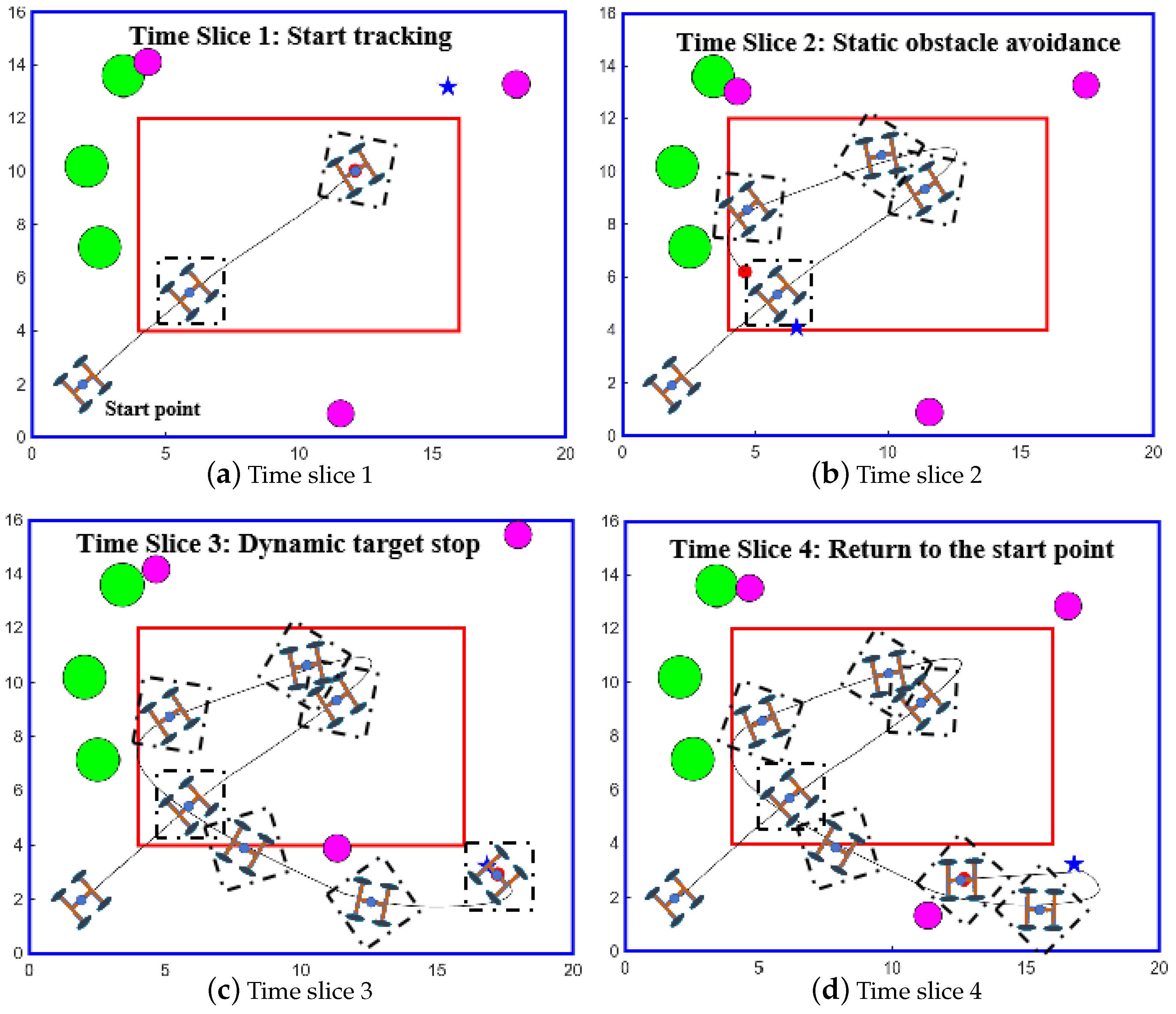Figure 4 presents four key time slices. In Figure 4a, the AUGV initiates from the starting point to track the dynamic target upon task activation. The AUGV proactively avoids collisions near static obstacles, as shown in Figure 4b. After the dynamic target stops, the AUGV returns to the starting point from the stopping position. Notably, the vehicle also proactively triggers collision avoidance when encountering dynamic obstacles, thereby ensuring the safe execution of the task.

To more clearly demonstrate the dynamic target tracking performance, Figure 5 provides a detailed view of the position tracking. Specifically, the further the AUGV is from the target, the faster its speed. Due to the unpredictability of the speed of the dynamic target and movement direction changes, the AUGV continuously adjusts its motion until it tracks the target and then returns to the starting point at a constant speed once the target stops. It is worth mentioning that Figure 5 shows two interesting phenomena. Firstly, the AUGV cannot predict the motion trajectory of dynamic targets and can only obtain the position information based on the indoor positioning system. When the target moves in a straight line, the distance between the UAGV and the target gradually shortens. When the target suddenly changes direction, the AUGV will adjust the direction of motion in a timely manner to achieve fast tracking. Secondly, when the target suddenly changes its motion state, there may be a situation where the car intersects with the target. For example, at 17 s, the UAGV meets the target, but at this time, the UAGV does not stop but continues to track until the target is stationary. After tracking to a stationary target, the UAGV will default to a constant speed and return to the starting point to wait for the next task. Figure 6 showcases the changes in tracking speed, we can see that the speed of the dynamic target gradually decreases to 0, but the speed of the UAGV will have significant fluctuations. The main reason is that the target will experience a rebound phenomenon after touching the boundary, resulting in a sudden change in the direction of motion, which in turn leads to a sudden change in the distance between the AUGV and the target. During normal tracking, the distance between the AUGV and the target decreases, and the speed of the AUGV also decreases. When the distance increases, the speed of the AUGV will increase to achieve fast tracking.

Subsequently, we conducted simulations for two typical scenarios, as shown in Figure 7. In Scenario 1, under a safe environment, the proposed dynamic target tracking control algorithm achieves smooth and stable tracking performance. Specifically, the AUGV will adjust speed and direction of motion in a timely manner based on the position changes of the dynamic target to ensure tracking performance. After tracking until the target stops, the AUGV will return to the starting point at a constant speed. In Scenario 2, within a congested obstacle environment, the algorithm effectively and accurately tracks the dynamic target. Specifically, the AUGV ensures tracking performance for dynamic targets while safely avoiding static and dynamic obstacles. Meanwhile, the AUGV exhibits an interesting phenomenon when a dynamic obstacle suddenly blocks the movement of the AUGV, the AUGV will temporarily stop and wait for the obstacle to move out of the safe range.

We conducted comparative simulations in both safe and obstacle-laden environments, as illustrated in Figure 8. The simulation results clearly demonstrate that the proposed tracking control strategy outperforms the finite-time TSM tracking strategy [37] and the Backstepping tracking strategy [38]. We can clearly see that the finite-time TSM tracking strategy has higher tracking accuracy, but the motion stability of the AUGV is too poor. For the Backstepping tracking strategy, although the tracking trajectory is smooth, the tracking accuracy is not ideal. Finally, Figure 9 clearly verifies that the proposed FTESO effectively enables precise observation and compensation for unknown disturbances in the tracking control system. Specifically, we can see that without adding FTESO, the fluctuation of the tracking controller is significantly affected by the lumped disturbance term. After observing and compensating for the lumped disturbance term through FTESO, the controller input becomes much smoother.

6. Conclusions

This paper addresses the precise tracking control of a dynamically moving target for the underactuated AUGV under dynamic and static obstacle constraints, aiming to enhance the operational efficiency of physical education auxiliary unmanned ground vehicle. In the guidance layer, position constraints based on an exponential stability Lyapunov function and safety constraints using control barrier functions (ES-CBF) are designed. The desired cooperative velocity guidance law for the AUGV is solved through quadratic programming. Based on the designed cooperative velocity, the desired heading angle is provided, leading to the design of the angular velocity guidance law for the AUGV. In the control layer, a nonlinear tracking differentiator (NLTD) is introduced to estimate the derivative of the velocity guidance signal within a finite time. A fixed-time extended state observer (FTESO) is designed to estimate disturbances and track the given velocity using a fixed-time control law. Simulation results verify the effectiveness of the proposed target tracking controller and the collision avoidance controller. Future research will further expand to irregular sports venues and obstacle constraints, and conduct multi-target tracking physical platform verification when experimental conditions are mature.

References

1. Dinelli, C.; Racette, J.; Escarcega, M.; Lotero, S.; Gordon, J.; Montoya, J.; Dunaway, C.; Androulakis, V.; Khaniani, H.; Shao, S.; et al. Configurations and Applications of Multi-Agent Hybrid Drone/Unmanned Ground Vehicle for Underground Environments: A Review. Drones 2023, 7, 136. [Google Scholar] [CrossRef]
2. Rondelli, V.; Franceschetti, B.; Mengoli, D. A Review of Current and Historical Research Contributions to the Development of Ground Autonomous Vehicles for Agriculture. Sustainability 2022, 14, 9221. [Google Scholar] [CrossRef]
3. Ahmad Sidi, M.H.; Hudha, K.; Kadir, Z.A.; Akhimullah Subari, M.; Amer, N.H.; Fairuz Syed Mohd Dardin, S. Speed Tracking Control of Tracked Vehicle using PID Controller Optimized by Particle Swarm Optimization. In Proceedings of the 2020 IEEE International Conference on Automatic Control and Intelligent Systems (I2CACIS), Shah Alam, Malaysia, 20 June 2020; pp. 107–111. [Google Scholar] [CrossRef]
4. Yao, D.; Li, H.; Lu, R.; Shi, Y. Distributed Sliding-Mode Tracking Control of Second-Order Nonlinear Multiagent Systems: An Event-Triggered Approach. IEEE Trans. Cybern. 2020, 50, 3892–3902. [Google Scholar] [CrossRef]
5. Köhler, J.; Soloperto, R.; Müller, M.A.; Allgöwer, F. A Computationally Efficient Robust Model Predictive Control Framework for Uncertain Nonlinear Systems. IEEE Trans. Autom. Control 2021, 66, 794–801. [Google Scholar] [CrossRef]
6. Wang, N.; Gao, Y.; Zhao, H.; Ahn, C.K. Reinforcement Learning-Based Optimal Tracking Control of an Unknown Unmanned Surface Vehicle. IEEE Trans. Neural Netw. Learn. Syst. 2020, 32, 3034–3045. [Google Scholar] [CrossRef]
7. Lin, H.Y.; Peng, X.Z. Autonomous Quadrotor Navigation with Vision-Based Obstacle Avoidance and Path Planning. IEEE Access 2021, 9, 102450–102459. [Google Scholar] [CrossRef]
8. Zhao, Z.; Zhu, B.; Zhou, Y.; Yao, P.; Yu, J. Cooperative Path Planning of Multiple Unmanned Surface Vehicles for Search and Coverage Task. Drones 2022, 7, 21. [Google Scholar] [CrossRef]
9. Zhang, J.X.; Yang, T.; Chai, T. Neural Network Control of Underactuated Surface Vehicles with Prescribed Trajectory Tracking Performance. IEEE Trans. Neural Netw. Learn. Syst. 2022, 35, 8026–8039. [Google Scholar] [CrossRef] [PubMed]
10. Du, B.; Yang, K.; Zhang, W.; Chen, H. Terminal Line-of-Sight Angle-Constrained Target Tracking Guidance for Unmanned Surface Vehicles. IEEE Trans. Veh. Technol. 2024, 73, 12515–12529. [Google Scholar] [CrossRef]
11. Bibuli, M.; Odetti, A.; Zereik, E. Adaptive Steering Control for an Azimuth Thrusters-Based Autonomous Vessel. J. Mar. Eng. Technol. 2020, 19 (Suppl. 1), 76–91. [Google Scholar] [CrossRef]
12. Zuo, Z.; Yang, X.; Li, Z.; Wang, Y.; Han, Q.; Wang, L.; Luo, X. MPC-Based Cooperative Control Strategy of Path Planning and Trajectory Tracking for Intelligent Vehicles. IEEE Trans. Intell. Veh. 2020, 6, 513–522. [Google Scholar] [CrossRef]
13. Masnavi, H.; Adajania, V.K.; Kruusamäe, K.; Singh, A.K. Real-Time Multi-Convex Model Predictive Control for Occlusion-Free Target Tracking with Quadrotors. IEEE Access 2022, 10, 29009–29031. [Google Scholar] [CrossRef]
14. Yan, D.; Zhang, W.; Chen, H. Design of a Multi-Constraint Formation Controller Based on Improved MPC and Consensus for Quadrotors. Aerospace 2022, 9, 94. [Google Scholar] [CrossRef]
15. Mobayen, S.; Mofid, O.; Din, S.U.; Bartoszewicz, A. Finite-Time Tracking Controller Design of Perturbed Robotic Manipulator Based on Adaptive Second-Order Sliding Mode Control Method. IEEE Access 2021, 9, 71159–71169. [Google Scholar] [CrossRef]
16. Cervantes-Rojas, J.S.; Muñoz, F.; Chairez, I.; González-Hernández, I.; Salazar, S. Adaptive Tracking Control of an Unmanned Aerial System Based on a Dynamic Neural-Fuzzy Disturbance Estimator. ISA Trans. 2020, 101, 309–326. [Google Scholar] [CrossRef]
17. Karami, H.; Alattas, K.A.; Mobayen, S.; Fekih, A. Adaptive Integral-Type Terminal Sliding Mode Tracker Based on Active Disturbance Rejection for Uncertain Nonlinear Robotic Systems with Input Saturation. IEEE Access 2021, 9, 129528–129538. [Google Scholar] [CrossRef]
18. Sekban, H.T.; Başçi, A. Performing Trajectory Tracking Control of an Unmanned Ground Vehicle Using Fractional Order Terminal Sliding Mode Controller. Int. J. Sustain. Aviat. 2023, 9, 73–88. [Google Scholar] [CrossRef]
19. Zhang, L.; Jiang, Y.; Chen, G.; Tang, Y.; Lu, S.; Gao, X. Heading Control of Variable Configuration Unmanned Ground Vehicle Using PID-Type Sliding Mode Control and Steering Control Based on Particle Swarm Optimization. Nonlinear Dyn. 2023, 111, 3361–3378. [Google Scholar] [CrossRef]
20. Jiang, Y.; Xu, X.; Zhang, L. Heading Tracking of 6WID/4WIS Unmanned Ground Vehicles with Variable Wheelbase Based on Model-Free Adaptive Control. Mech. Syst. Signal Process. 2021, 159, 107715. [Google Scholar] [CrossRef]
21. Cheng, W.; Jiang, B.; Zhang, K.; Ding, S.X. Robust Finite-Time Cooperative Formation Control of UGV-UAV with Model Uncertainties and Actuator Faults. J. Frankl. Inst. 2021, 358, 8811–8837. [Google Scholar] [CrossRef]
22. Hassan, N.; Saleem, A. Neural Network-Based Adaptive Controller for Trajectory Tracking of Wheeled Mobile Robots. IEEE Access 2022, 10, 13582–13597. [Google Scholar] [CrossRef]
23. Wu, Y.; Li, C.; Yuan, C.; Li, M.; Li, H. Predictive Control for Small Unmanned Ground Vehicles via a Multi-Dimensional Taylor Network. Appl. Sci. 2022, 12, 682. [Google Scholar] [CrossRef]
24. Sui, Y.; Yang, Z.; Zhuo, H.; You, Y.; Que, W.; He, N. A Fuzzy Pure Pursuit for Autonomous UGVs Based on Model Predictive Control and Whole-Body Motion Control. Drones 2024, 8, 554. [Google Scholar] [CrossRef]
25. Chen, T.; Zhao, R.; Chen, J.; Zhang, Z. Data-Driven Active Disturbance Rejection Control of Plant-Protection Unmanned Ground Vehicle Prototype: A Fuzzy Indirect Iterative Learning Approach. IEEE/CAA J. Autom. Sinica 2024, 11, 1892–1894. [Google Scholar] [CrossRef]
26. Lu, S.; Jiang, Y.; Xu, X.; Qian, H.; Zhang, W. Adaptive Heading Control Strategy for Unmanned Ground Vehicle with Variable Wheelbase Based on Robust-Active Disturbance Rejection Control. Control Eng. Pract. 2024, 142, 105786. [Google Scholar] [CrossRef]
27. Wang, H.; Zuo, Z.; Xue, W.; Wang, Y.; Yang, H. Switching Longitudinal and Lateral Semi-Decoupled Active Disturbance Rejection Control for Unmanned Ground Vehicles. IEEE Trans. Ind. Electron. 2023, 71, 3034–3043. [Google Scholar] [CrossRef]
28. Gu, N.; Peng, Z.; Wang, D.; Shi, Y.; Wang, T. Anti-Disturbance Coordinated Path Following Control of Robotic Autonomous Surface Vehicles: Theory and Experiment. IEEE/ASME Trans. Mechatronics 2019, 24, 2386–2396. [Google Scholar] [CrossRef]
29. Liu, L.; Wang, D.; Peng, Z.; Chen, C.P.; Li, T. Bounded Neural Network Control for Target Tracking of Underactuated Autonomous Surface Vehicles in the Presence of Uncertain Target Dynamics. IEEE Trans. Neural Netw. Learn. Syst. 2018, 30, 1241–1249. [Google Scholar] [CrossRef]
30. Peng, Z.H.; Wang, J.; Han, Q.L. Path-Following Control of Autonomous Underwater Vehicles Subject to Velocity and Input Constraints via Neurodynamic Optimization. IEEE Trans. Ind. Electron. 2019, 66, 8724–8732. [Google Scholar] [CrossRef]
31. Peng, Y.; Li, Y. Autonomous Trajectory Tracking Integrated Control of Unmanned Surface Vessel. J. Mar. Sci. Eng. 2023, 11, 568. [Google Scholar] [CrossRef]
32. Ames, A.D.; Xu, X.; Grizzle, J.W.; Tabuada, P. Control Barrier Function Based Quadratic Programs for Safety Critical Systems. IEEE Trans. Autom. Control. 2016, 62, 3861–3876. [Google Scholar] [CrossRef]
33. Kolathaya, S.; Ames, A.D. Input-to-State Safety with Control Barrier Functions. IEEE Control. Syst. Lett. 2019, 3, 108–113. [Google Scholar] [CrossRef]
34. Yi, S.; Wang, J.; Li, B. Composite Backstepping Control with Finite-Time Convergence. Optik 2017, 142, 260–272. [Google Scholar] [CrossRef]
35. Liu, H.; Peng, Z.; Gu, N.; Wang, H.; Liu, L.; Wang, D. Collision-Free Automatic Berthing of Maritime Autonomous Surface Ships via Safety-Certified Active Disturbance Rejection Control. ISA Trans. 2024, 148, 24–31. [Google Scholar] [CrossRef]
36. Garg, K.; Panagou, D. Characterization of Domain of Fixed-Time Stability under Control Input Constraints. In Proceedings of the 2021 American Control Conference (ACC), New Orleans, LA, USA, 25–28 May 2021; IEEE: Piscataway, NJ, USA, 2021; pp. 2272–2277. [Google Scholar]
37. Xu, J.; Fang, L.; Wang, H.; Zhao, Q.; Wan, Y.; Gao, Y. Observer-Based Finite-Time Prescribed Performance Sliding Mode Control of Dual-Motor Joints-Driven Robotic Manipulators with Uncertainties and Disturbances. Actuators 2024, 13, 325. [Google Scholar] [CrossRef]
38. Li, J.; Li, X.; Lu, J.; Cao, B.; Sun, J. A Novel Robust Hybrid Control Strategy for a Quadrotor Trajectory Tracking Aided with Bioinspired Neural Dynamics. Appl. Sci. 2024, 14, 9592. [Google Scholar] [CrossRef]
Figure 1. Typical dynamic target tracking scenario and motion model of the AUGV. (a). The application of the AUGV in the tennis. (b). The mathematical model of the AUGV.
Electronics 13 04620 g001
Figure 2. The framework of target tracking control.
Electronics 13 04620 g002
Figure 3. Global tracking diagram.
Electronics 13 04620 g003
Figure 4. Local tracking diagram. (a) Start tracking; (b) static obstacle avoidance; (c) dynamic target stop; (d) return to the start point.
Electronics 13 04620 g004
Figure 5. Position tracking diagram.
Electronics 13 04620 g005
Figure 6. Velocity tracking diagram.
Electronics 13 04620 g006
Figure 7. Other typical scenarios. (a) Scenario without obstacles. (b) Scenario with many obstacles.
Electronics 13 04620 g007
Figure 8. Comparison of target tracking performance. (a) Scenario without obstacles. (b) Scenario with many obstacles.
Electronics 13 04620 g008
Figure 9. Comparison of the disturbance observer performance.
Electronics 13 04620 g009
Disclaimer/Publisher’s Note: The statements, opinions and data contained in all publications are solely those of the individual author(s) and contributor(s) and not of MDPI and/or the editor(s). MDPI and/or the editor(s) disclaim responsibility for any injury to people or property resulting from any ideas, methods, instructions or products referred to in the content.