Graph Neural Network-Based Speech Emotion Recognition: A Fusion of Skip Graph Convolutional Networks and Graph Attention Networks

Abstract

In speech emotion recognition (SER), our research addresses the critical challenges of capturing and evaluating node information and their complex interrelationships within speech data. We introduce Skip Graph Convolutional and Graph Attention Network (SkipGCNGAT), an innovative model that combines the strengths of skip graph convolutional networks (SkipGCNs) and graph attention networks (GATs) to address these challenges. SkipGCN incorporates skip connections, enhancing the flow of information across the network and mitigating issues such as vanishing gradients, while also facilitating deeper representation learning. Meanwhile, the GAT in the model assigns dynamic attention weights to neighboring nodes, allowing SkipGCNGAT to focus on both the most relevant local and global interactions within the speech data. This enables the model to capture subtle and complex dependencies between speech segments, thus facilitating a more accurate interpretation of emotional content. It overcomes the limitations of previous single-layer graph models, which were unable to effectively represent these intricate relationships across time and in different speech contexts. Additionally, by introducing a pre-pooling SkipGCN combination technique, we further enhance the ability of the model to integrate multi-layer information before pooling, improving its capacity to capture both spatial and temporal features in speech. Furthermore, we rigorously evaluated SkipGCNGAT on the IEMOCAP and MSP-IMPROV datasets, two benchmark datasets in SER. The results demonstrated that SkipGCNGAT consistently achieved state-of-the-art performance. These findings highlight the effectiveness of the proposed model in accurately recognizing emotions in speech, offering valuable insights and a solid foundation for future research on capturing complex relationships within speech signals for emotion recognition.

1. Introduction

Speech emotion recognition (SER) is a vital component of a multitude of applications, including human–computer interaction (HCI) [1], customer service [2], mental health monitoring [3], and educational tools [4]. The capacity to accurately discern emotions from speech can markedly enhance the user experience in interactive systems, facilitating more empathetic and responsive communication. Furthermore, for mental healthcare, SER can facilitate early detection and monitoring of emotional states, thereby providing valuable insights for timely intervention.

A substantial body of research has highlighted the pivotal role of SER in these domains. Schuller et al. [5] proposed a novel approach that integrates acoustic and linguistic features to achieve robust automatic emotion recognition. By integrating various classification techniques, including support vector machines (SVMs) and belief networks, their work demonstrated how acoustic features and spoken content can be effectively utilized to efficiently classify different emotional states.

Similarly, Eyben et al. [6] introduced the openSMILE toolkit, which supports various audio feature extraction techniques and has become essential for speech processing and music information retrieval. It can extract low-level descriptors, such as pitch, loudness, and spectral features, as well as higher-level functionals, such as statistical moments and delta coefficients. This versatility has made openSMILE a valuable tool for emotion recognition, speaker identification, and paralinguistic analysis [7,8]. For instance, the ability of a toolkit to extract features such as MFCCs, jitter, and shimmers has proven crucial in both automatic speech recognition and the detection of emotional nuances in speech [9,10]. These studies highlight the approach comprehensive feature extraction can use to significantly enhance SER performance, making it more efficient and adaptable to various applications.

In mental health, Cummins et al. [3] conducted a review of the use of speech analysis as an objective predictor of depression and suicide. Their study emphasized the importance of language as a key marker of these disorders and discussed how changes in language characteristics can be used as indicators of mental health issues. This review highlights the potential of SER to assist in the early diagnosis and monitoring of depression and suicide, while also identifying challenges and future directions and exploring emotion pair-based frameworks to improve SER performance.

For instance, in the work by Xi Ma et al. [11], an innovative approach was introduced that constructs more discriminative feature subspaces for every two different emotions (emotion-pair) to generate precise emotion bi-classification results. This method leverages the observation that some archetypal emotions are closer to the dimensional emotion space than others. To capture this emotion distribution information, a naive Bayes classifier-based decision fusion strategy was proposed, which demonstrated significant improvements in emotion recognition tasks.

Additionally, researchers have advanced this field by employing deep recurrent neural networks (RNNs) with local attention mechanisms. Ma et al. [12] applied deep RNNs to automatically discover emotionally relevant features from speech, enhancing the accuracy of emotion recognition by focusing on the emotionally salient regions of a speech signal.

Moreover, the introduction of segment-level feature representation combined with multiple instance learning [13] (MIL) for utterance-level SER is another significant development. In their 2019 study, Mao et al. [14] demonstrated the approach used by segment-level decisions to provide richer emotional information than traditional low-level descriptors, with deep neural network architectures, such as SegMLP and SegCNN outperforming manual feature extraction methods.

However, SER faces several challenges. Traditional SER methods rely on manually extracted speech features, such as spectrograms and Mel-frequency cepstrum coefficients (MFCCs) [15]. These features are typically classified using statistical methods or machine learning algorithms (e.g., SVMs and hidden Markov models) [16]. Gaussian mixture models (GMM) and hidden Markov models (HMMs) are widely used in SER [5]. These models offer advantages in processing time-series data and modeling the statistical properties of speech signals [6]. With the development of deep learning, CNNs and RNNs have been widely used for SER [12]. Deep learning models can learn emotion features automatically and perform well in complex emotion recognition tasks [14]. Naoumi et al. [17] proposed a deep learning solution leveraging complex neural networks, demonstrating that the deep learning-based approach can achieve performance comparable to traditional parameterized methods, with significantly lower computational complexity. Huiyun Zhang et al. [18] proposed a heterogeneous parallel convolutional Bi-LSTM model to address the effectiveness of feature extraction.

Recently, GNNs have gained considerable attention because of their ability to model complex relational data [19,20,21]. This has led to their increasing application in various domains, including SER. GNNs are particularly effective for SER because they can capture the intricate relationships between different speech segments, which are crucial for accurately identifying emotions. Many GNNs have been successfully applied in the SER field. For instance, Kipf et al. [19] introduced the concept of semi-supervised classification with graph convolutional networks (GCNs), which have since been adapted for SER tasks to enhance performance. Shirian et al. [20] proposed a compact graph architecture specifically designed for efficient and scalable speech emotion recognition and demonstrated significant improvements over traditional methods. Furthermore, Liu et al. [22] proposed a novel SER model called LSTMGIN, which employs a graph isomorphism network (GIN) on LSTM outputs to model global emotions in a non-Euclidean space. Liu et al. [23] cast the SER problem as a graph classification task by transforming variable-length utterances into graphs to avoid padding or cutting. Yan et al. [24] used a bidirectional long short-term memory (Bi-LSTM) network to capture long-term dependencies within speech features, allowing deeper frame-level emotion representations to be learned.

In addition, GNNs have been extensively applied in conversational emotion recognition. These models [25,26,27,28] were used to capture the intricate dependencies and contextual information present in multi-turn conversations. By representing a conversation as a graph, where nodes correspond to utterances and edges represent interactions or contextual links, GNNs can effectively model the dynamic flow of emotions throughout a conversation [25,26]. This approach can improve the accuracy and robustness of emotion recognition in conversation systems [27], paving the way for more empathetic and context-aware HCIs. This has significant implications for SER research, as the methodologies and insights gained from conversation emotion recognition can be leveraged to enhance the understanding and modeling of emotional dynamics in speech [28]. Zhang et al. [29] introduced the use of graph attention networks (GATs) in conversation emotion recognition, where the model assigns varying attention weights to different utterances based on their emotional relevance. These graph models in conversation emotion recognition have important reference significance for the field of speech emotion recognition.

Although previous models have achieved significant success, they often rely on a single GNN architecture, which limits their ability to capture the full spectrum of complex and dynamic interactions within speech data. To illustrate, when utilizing GCNs [19,20] for the processing of graph structure data, the primary consideration is the neighborhood information of the nodes, which may result in an inability to effectively capture long-distance dependencies, thus affecting the extraction of complex speech features. Moreover, when employing GAT [29] for the processing of graph structure, it focuses more on the correlation between nodes and ignores the overall structural information of the graph, which may lead to an insufficient understanding of the speech signal as a whole. Inspired by the approaches in these studies [20,30,31,32], we propose a hybrid model, SkipGCNGAT and SkipGCNGAT, which integrate the strengths of both skip graph convolutional networks (SkipGCNs) and GATs to address these challenges. The motivation behind SkipGCNGAT stems from the need to develop a more comprehensive architecture that addresses the limitations of previous approaches. By combining ability of SkipGCNs to capture local information with attention mechanism of GATs, SkipGCNGAT effectively integrates both local and global perspectives. This allows the model to dynamically prioritize relevant information, improving its capacity to handle complex relationships and varying contextual importance in speech emotion recognition tasks.

By combining these two architectures, SkipGCNGAT can capture the full range of relationships within the speech data more effectively. SkipGCN contributes to the stable propagation of information across layers, mitigating issues such as gradient vanishing and ensuring that deeper network architectures remain effective. Simultaneously, GATs provide flexibility to assign attention weights to different nodes, enabling the model to prioritize the most emotionally salient aspects of speech signals. This dual approach offers a more comprehensive understanding of the emotional states conveyed through speech, as it allows the model to integrate fine-grained local features and a broader global context.

2. Skip Graph Convolutional and Graph Attention Network

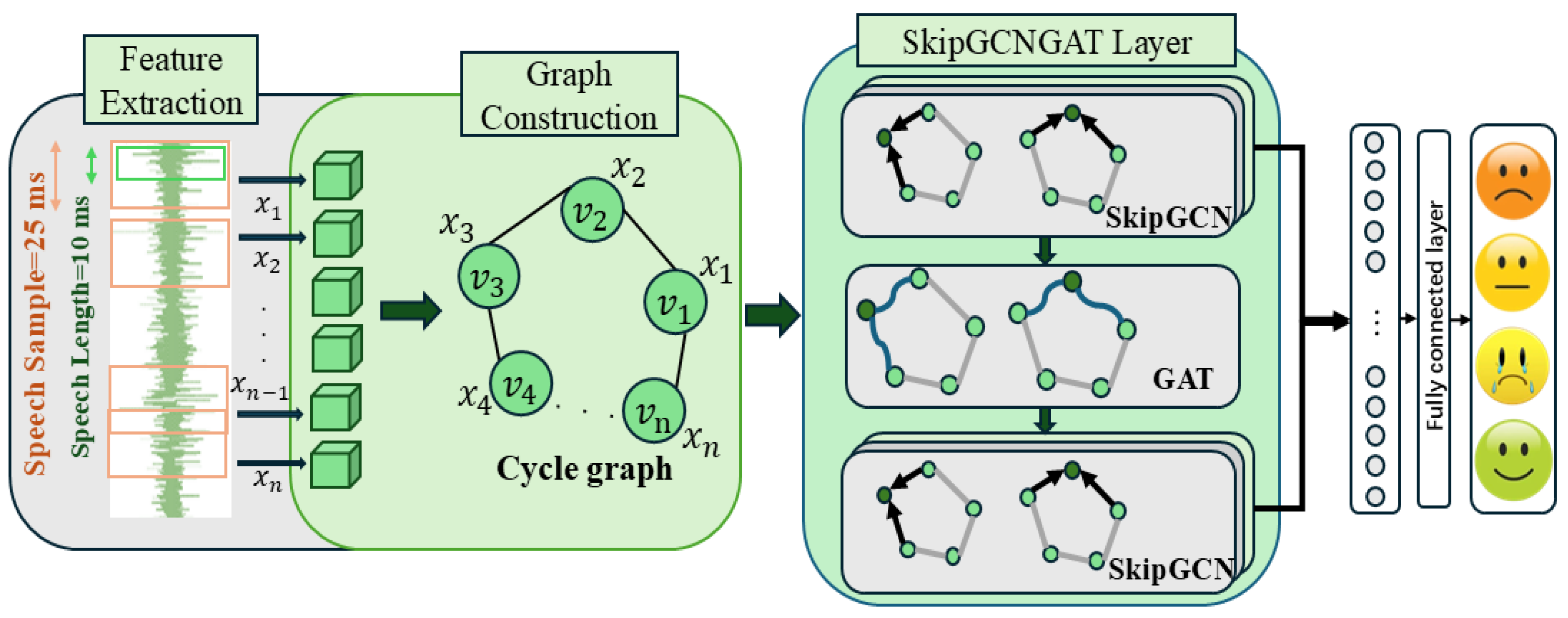
In this section, we introduce the overall process of SkipGCNGAT. Figure 1 illustrates the architecture and process flow of SkipGCNGAT, including speech preprocessing, the main SkipGCN and GAT layers, and the final hybrid prediction layer.

Initially, we utilized the openSMILE 3.0 toolkit [6] to extract low-level descriptors (LLDs) from the speech signal, which are denoted by $x_n$ and serve as node representations. Based on this study [20], these nodes were then used to construct a cycle graph in which each node captured the temporal and acoustic properties of the speech segments, preserving both local and sequential dependencies.

Following feature extraction and graph construction, the graph data were processed using the SkipGCNGAT layer, which is a three-layer network designed to capture complex relationships in speech data. This network includes two SkipGCN modules and a GAT [30] layer. Figure 2 illustrates the process of SkipGCN, which combines a GCN and multi-layer perceptron (MLP) integrated with skip connections, capturing both local and global information. The GCN aggregates information from neighboring nodes, producing features denoted as $z_n$, whereas the MLP applies nonlinear transformations, producing higher-level features denoted as $y_n$. Skip connections preserve the original input features $x_n$, ensuring robust gradient flow and preventing vanishing gradients.

Subsequently, the refined features are passed to the GAT layer, which assigns varying attention scores to the edges between nodes. This enables the model to dynamically prioritize and amplify the influence of the most relevant nodes and connections, thereby ensuring that the relationships critical to emotion recognition are given greater weight during the learning process. This targeted focus allows the model to capture subtle emotional cues more effectively by emphasizing the most informative parts of the graph.

The final SkipGCN module further refines and consolidates the features using the same combination of GCN and MLP. The outputs from this layer are refined through skip connections, which preserve and integrate both the original input and newly learned features. Inspired by this study [32], features from both SkipGCN modules were combined and passed through a sum-pooling operation and a fully connected layer, producing the final emotion prediction based on the comprehensive analysis performed by the SkipGCNGAT model.

2.1. Feature Extraction

We used OpenSMILE [6] to extract low-level descriptors (LLDs) from speech utterances. The feature set includes Mel-frequency cepstral coefficients (MFCCs) [33], the zero-crossing rate, voice probability, fundamental frequency (F0), and frame energy. The input settings were configured with mono output (monoMixdown = 1), frame size of 0.025 s (25 ms), and frame step of 0.010 s (10 ms). In the preprocessing phase, pre-emphasis was applied with a coefficient $k=0.97$ using the cVectorPreemphasis function, and a Hamming window function (winFunc = ham) was used to reduce spectral leakage [34]. These extracted features are subsequently smoothed using a moving average filter, and the smoothed values are used to calculate the first-order delta coefficients [35]. We then utilized these extracted and processed features as nodes when constructing cycle graphs. Each feature vector, representing a specific timeframe of the speech signal, serves as a node in the graph, allowing us to capture both the temporal dynamics and relationships between consecutive speech frames. By connecting these nodes in a cyclical structure, we effectively modeled the sequential dependencies and interactions inherent to the speech signal. This graph-based representation enables a more comprehensive analysis as it preserves the continuity of speech while also facilitating the extraction of meaningful patterns and relationships across the entire utterance.

2.2. Graph Construction

In this approach to speech signal processing, each utterance is converted into a graphical representation by creating a graph denoted by $G=\left(V,E\right)$, where V is a collection of M nodes, represented as $\left\{V_i\right\}$ for i, ranging from 1 to M, and E is the ensemble of edges that interconnect these nodes. The connectivity within this graph is encapsulated by the adjacency matrix A, which resides in the space of real numbers $R^{M\times M}$. The element $A_{ij}$ in this matrix indicates whether there is a connection between nodes $V_i$ and $V_j$.

The graph is constructed by assigning each of the M frames of the speech signal, which are brief overlapping segments, to a node in the graph [36]. As depicted in the matrix, this method provides the direct mapping from the speech signal to the graph structure. Because the speech data do not determine the graph’s architecture, inspired by [20] we deliberately opt for a cyclic graph configuration characterized by the adjacency matrix $A_c$.

The cyclic adjacency matrix $A_c$ is structured as follows:

$$A_c=\left[\begin{array}{ccccc}0& 1& 0& \cdots & 1\\ 1& 0& 1& \cdots & 0\\ 0& 1& 0& \cdots & 0\\ ⋮& ⋮& ⋮& \ddots & ⋮\\ 1& 0& 0& \cdots & 0\end{array}\right]$$

(1)

The cyclic graph structure enables continuous information flow between nodes, effectively capturing the sequential and repetitive nature of speech signals. This structure ensures that the start and end of the temporal sequence are connected, facilitating seamless information propagation. It is particularly effective in modeling circular dependencies and temporal dynamics in speech data. Additionally, the cyclic arrangement offers benefits due to the special properties of its graph Laplacian, which streamlines spectral computations in GCNs [37], enhancing the ability of model to process speech data. Each node $V_i$ is associated with a feature vector $H_i$ that belongs to the space of real numbers ${\mathbb{R}}^p$. These vectors encapsulate LLDs extracted from the corresponding segments of the speech signal. When aggregated, these feature vectors form the feature matrix H, which resides in ${\mathbb{R}}^{M\times P}$, and is defined as $H=\left[H_1,\cdots ,H_M\right]$.

2.3. Graph Fusion: Integrating SkipGCN and GAT Modules

2.3.1. Skip Graph Convolutional Network (SkipGCN)

The graph Laplacian L is central to capturing the local structure of the graph. This is computed using the degree and adjacency matrices $\mathbf{A}$ [37]. The unnormalized graph Laplacian is defined as

$$\mathcal{L}=\mathbf{D}-\mathbf{A}$$

(2)

where $\mathbf{D}$ is a diagonal degree matrix with elements $D_{ii}={\Sigma }_j{A}_{ij}$, which represents the degree of node i. The adjacency matrix A encodes the connections between nodes, where $A_{ij}=1$ if there is an edge between nodes i and j and $A_{ij}=0$ otherwise.

In the normalized form, the graph Laplacian is expressed as follows:

$$\mathcal{L}={\mathbf{D}}^{-{\displaystyle \frac{1}{2}}}(\mathbf{D}-\mathbf{A}){\mathbf{D}}^{-{\displaystyle \frac{1}{2}}}=\mathbf{I}-{\mathbf{D}}^{-{\displaystyle \frac{1}{2}}}{\mathbf{AD}}^{-{\displaystyle \frac{1}{2}}}$$

(3)

where $\mathbf{I}$ denotes an identity matrix. This normalization helps stabilize the training process by ensuring that the eigenvalues of L are within a specific range, making the convolution operation more numerically stable [19,37].

When the Laplacian $\mathbf{L}$ is applied to the feature matrix $\mathbf{H}$, it aggregates the features of each node’s neighbors, weighted by the graph structure, resulting in a new feature matrix:

$$\widehat{\mathbf{H}}=\mathbf{LH}$$

(4)

Each row of $\mathbf{H}$ corresponds to the feature vector of a node, and the operation $\widehat{\mathbf{H}}=\mathbf{LH}$ produces a new feature matrix $\widehat{\mathbf{H}}$ where each node’s features are updated based on the features of its neighbors. This step ensures that the updated features incorporate the local structural information from the graph.

Following the aggregation, the feature matrix $\widehat{\mathbf{H}}$ undergoes a linear transformation by multiplying it by a learnable weight matrix $\mathbf{W}$:

$$\mathbf{Z}=\widehat{\mathbf{H}}\mathbf{W}=\mathbf{LHW}$$

(5)

$\mathbf{W}$ is a trainable matrix that maps the aggregated features to a new feature space. The calculation of the weight matrix $\mathbf{W}$ is a dynamic process, where the model continuously learns and adjusts its values through forward and backward propagation. This enables the model to effectively project the aggregated features into a higher-dimensional space, allowing it to better capture complex relationships and emotional information within the speech data. This multiplication allows the model to learn the optimal linear combination of features, projecting the aggregated information into a higher-dimensional space that is more suitable for capturing complex patterns.

The output of the linear transformation, $\mathbf{Z}$, is then passed through a nonlinear activation function $\sigma$ to introduce nonlinearity into the model.

$${\mathbf{H}}_{\mathrm{nonlinear}}=\sigma \left(\mathbf{Z}\right)=\sigma \left(\mathbf{LHW}\right)$$

(6)

The activation function $\sigma$ is ReLU (Rectified Linear Unit). ReLU helps the model capture complex patterns and effectively mitigates the vanishing gradient problem, enabling more efficient learning.

This is inspired by studies that applied GCN [25,31] to ResNet [38]. After the activation function is applied, the resulting feature matrix ${\mathbf{H}}_{\mathrm{nonlinear}}$ is added to the original input feature matrix $\mathbf{H}$, forming the skip connection in SkipGCN:

$${\mathbf{H}}_{\mathrm{skip}}={\mathbf{H}}_{\mathrm{nonlinear}}+\mathbf{H}=\sigma \left(\mathbf{LHW}\right)+\mathbf{H}$$

(7)

In this equation, ${\mathbf{H}}_{\mathrm{skip}}$ is the output feature matrix, resulting from the combination of the nonlinearly transformed features and the original input features via the skip connection. The skip connection aims to facilitate the flow of information across layers, particularly in deep networks, where it helps to prevent issues such as vanishing or exploding gradients. By directly adding the input features to the output features, the skip connection enhances model robustness and simplifies the optimization process, making deep networks easier to train.

After applying the GCN and a skip connection, the output ${\mathbf{H}}_{\mathrm{skip}}$ is fed into an MLP layer for further transformation [39]:

$${\mathbf{Z}}_{MLP}=\mathrm{MLP}\left({\mathbf{H}}_{\mathrm{skip}}\right)$$

(8)

where ${\mathbf{Z}}_{MLP}$ represents the output of the MLP layer. The MLP consists of multiple fully connected layers with nonlinear activation functions that further refine and transform the features.

Subsequently, a second skip connection is applied, which combines the output of the MLP with the input to the MLP (which is the output of the first skip connection).

$${\mathbf{H}}_{\mathrm{skip}}^{\prime }={\mathbf{Z}}_{MLP}+{\mathbf{H}}_{\mathrm{skip}}$$

(9)

Here, ${\mathbf{H}}_{\mathrm{skip}}^{\prime }$ denotes the final output, obtained by adding the MLP output ${\mathbf{Z}}_{MLP}$ to the original input ${\mathbf{H}}_{\mathrm{skip}}$ of the MLP layer. This skip connection ensures that the original features are retained while allowing the network to learn more complex transformations.

This process is repeated across all layers, resulting in the final output matrix ${\mathbf{H}}^{\prime }$:

$${\mathbf{H}}^{\prime }={\mathrm{SkipGCN}}_L(\dots \left({\mathrm{SkipGCN}}_2({\mathrm{SkipGCN}}_1\left({\mathbf{H}}^{\left(0\right)}\right))\dots )\right)$$

(10)

where ${\mathbf{H}}^{\left(0\right)}$ denotes the initial input feature matrix. ${\mathrm{SkipGCN}}_L(·)$ denotes the operation of the $L\mathrm{th}$ SkipGCN layer. ${\mathbf{H}}^{\prime }$ is the output feature matrix after the final SkipGCN layer L.

2.3.2. Graph Attention Network (GAT)

The output ${\mathbf{H}}^{\prime }$ from the MLP is used as the input to the GAT:

$${\mathbf{H}}^{″}=\mathrm{GAT}({\mathbf{H}}^{\prime },\mathbf{A})$$

(11)

where ${\mathbf{H}}^{″}$ is the node feature matrix updated by the GAT, and $\mathbf{A}$ is the adjacency matrix.

Each attention head uses the following mechanism [30] to compute the attention score $e_{ij}$ between nodes i and node j:

$$e_{ij}=\mathrm{LeakyReLU}\left({\overrightarrow{a}}^T[\mathbf{W}{h}_i\left|\right|\mathbf{W}{h}_j]\right)$$

(12)

Here, $\overrightarrow{a}$ is the learnable attention parameter, $\mathbf{W}$ is the weight matrix, and $h_i$ and $h_j$ are the feature representations of nodes i and j, respectively. The attention scores $e_{ij}$, which are calculated for the edge between nodes i and j, are then normalized using the SoftMax function to obtain the attention weights $a_{ij}$ [30]:

$$a_{ij}={\displaystyle \frac{exp\left(e_{ij}\right)}{{\sum }_{k\in N_i}exp\left(e_{ik}\right)}}$$

(13)

Here, $a_{ij}$ represents the attention weight between nodes i and j, which is calculated by normalizing the attention score $e_{ij}$ using the SoftMax function. $N_i$ denotes the set of neighboring nodes of node i. The term $exp\left(e_{ij}\right)$ is the exponential of the attention score, and ${\sum }_{k\in N_i}exp\left(e_{ik}\right)$ serves as the normalization factor that ensures that the weights sum to one.

These attention weights $a_{ij}$ are used to obtain a weighted sum of the features of neighboring nodes, which updates the features for node i across each attention head as follows:

$$h_i^{\prime }=\sigma \left(\sum _{j\in N_i}{a}_{ij}\mathbf{W}{h}_j\right)$$

(14)

Here, $\mathbf{W}$ is a learnable weight matrix that transforms the feature vectors before they are used to calculate the attention scores. The feature $h_j$ denotes the input feature vector associated with node j, a neighbor of node i. The attention weights $a_{ij}$ determine the importance of neighbor j’s feature when updating node i’s feature. $\sigma (·)$ is a nonlinear activation function applied to the weighted sum of features. It is worth noting that this approach assumes all neighboring features are relevant based on attention weights. However, due to the SoftMax attention mechanism, noise or irrelevant features might still influence the model, potentially affecting its overall performance.

For multi-head attention, the outputs from all attention heads are concatenated to form the final output for each node:

$$h_i^{″}{=\Vert }_{m=1}^M{h_i^{\prime }}^{\left(m\right)}$$

(15)

where M represents the number of attention heads and $h_i^{\prime \left(m\right)}$ is the output feature for node i from the $m\mathrm{th}$ attention head. This concatenation approach preserves the distinct information captured by each attention head, enriches the final node representations, and enables the model to better capture and emphasize the key structural dependencies and node interactions.

$${\mathbf{H}}^{″}=\left[\begin{array}{c}{h}_1^{″}\\ h_2^{″}\\ ⋮\\ h_N^{″}\end{array}\right]\in {\mathbb{R}}^{N\times F^{″}}$$

(16)

where N represents the number of nodes, $F^{″}=M\times F^{\prime }$ denotes the dimensionality of the concatenated feature vectors from all attention heads, with $F^{\prime }$ being the dimensionality of the output from each individual attention head. Each $h_i^{″}$ is the concatenated feature vector for node i, encapsulating information from all the attention heads.

2.3.3. Feature Integration and Transformation Process

After obtaining the multi-head attention output $H^{″}$, this feature matrix is then passed through a subsequent SkipGCN module. This module applies a graph convolution operation followed by an MLP to further refine the node features. The SkipGCN layer integrates a skip connection that combines the input and output features, preserving the original information, while allowing the model to learn more complex transformations. The resulting feature matrix from this layer is denoted as $H^{‴}$:

$${\mathbf{H}}^{‴}={\mathrm{SkipGCN}}_L(\dots ({\mathrm{SkipGCN}}_2\left({\mathrm{SkipGCN}}_1\left({\mathbf{H}}^{″}\right)\right)\dots ))$$

(17)

The number L of SkipGCN layers is selected dynamically based on the complexity of the dataset to prevent the model from becoming excessively deep. This adaptive strategy ensures that the model is appropriately tailored to the characteristics of the data being processed, optimizing both performance and generalization.

To capture more comprehensive features [32], the model then combines the outputs from the first and last SkipGCN layers.

$${\mathbf{H}}_{\mathrm{combined}}={\mathbf{H}}^{\prime }\oplus {\mathbf{H}}^{‴}$$

(18)

Here, the output ${\mathbf{H}}^{\prime }$ from the first SkipGCN layer is combined with ${\mathbf{H}}^{‴}$, the output from the final SkipGCN layer, to produce a unified feature representation ${\mathbf{H}}_{\mathrm{combined}}$. This combination is typically performed using an element-wise operation such as addition or concatenation, denoted by ⊕.

By integrating the initial and final feature transformations, this approach ensures that the model learns both the essential structural characteristics and more intricate patterns captured through the deeper layers. The combined feature matrix ${\mathbf{H}}_{\mathrm{combined}}$ thus provides a more holistic representation of the node features, facilitating an improved performance in downstream tasks.

Finally, the combined feature matrix ${\mathbf{H}}_{\mathrm{combined}}$ is aggregated using a sum-pooling operation to generate a global feature vector. This vector is then passed through a classifier to produce the final output.

$$\mathrm{Output}={\mathrm{Linear}}_3(\dots \left(\mathrm{sumpool}\left({\mathbf{H}}_{\mathrm{combined}}\right)\right))$$

(19)

During this process, ${\mathbf{H}}_{\mathrm{combined}}$ undergoes a series of linear transformations. Each linear transformation was followed by batch normalization and ReLU activation. Batch normalization normalizes the output of each linear layer, which helps stabilize and accelerate the training process. The final linear layer in the sequence produces the output of the model.

3. Experiments and Results

3.1. Datasets

In this subsection, the databases used in the experiments of this paper for both IEMOCAP [40] and MSP-IMPROV [41] will be introduced.

3.1.1. IEMOCAP Database

The interactive emotional dyadic motion capture (IEMOCAP) database has been extensively used in speech emotion recognition tasks. For the speech modality, the dataset [40] contains high-quality audio recordings of dyadic interactions between actors, annotated with both categorical emotions (such as anger, happiness, sadness, and neutrality). Speech data spanned 12 h, ensuring a range of naturalistic emotional expressions.

This dataset provides a rich resource for analyzing how emotional content affects speech patterns, including variations in pitch, tone, speed, and intensity. Researchers have leveraged speech data to train models to recognize emotions based on these acoustic features. In the experiments, 4490 speech samples were selected to maintain consistency with a previous study [20], with 1103 instances of anger, 595 instances of happiness, 1708 instances of neutrality, and 1084 instances of sadness.

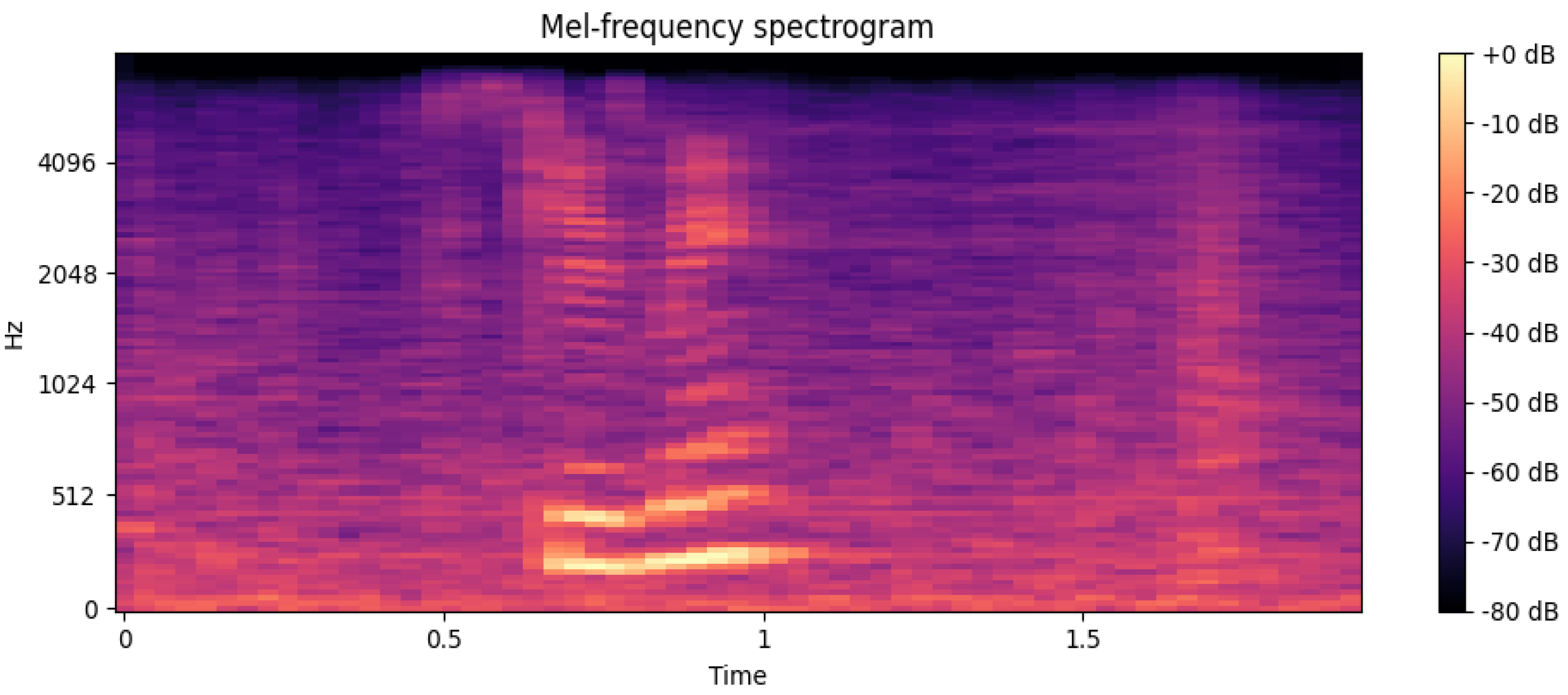
Figure 3 shows the Mel-frequency spectrogram of a sample from the IEMOCAP database. The spectrogram illustrates how speech energy is distributed across different frequency bands over time, which serves as the basis for extracting features such as MFCCs that are crucial for emotion recognition tasks.

3.1.2. MSP-IMPROV Database

The MSP-IMPROV dataset [41] is a valuable speech dataset designed for emotion perception studies. In contrast to traditional acted corpora, MSP-IMPROV includes improvised emotional dialogues that sound more natural, while maintaining controlled lexical content. Speech data were annotated using emotional labels focusing on four primary categories: anger, joy, sadness, and neutrality.

Speech recordings from MSP-IMPROV allow for a detailed study of how emotions influence speech articulation, prosody, and intonation in real-time dialogues. In total, 7798 utterances were used in the experiments, including 792 for anger, 3477 for neutrality, 885 for sadness, and 2644 for joy. The emotional diversity and naturalism of speech data make MSP-IMPROV an ideal resource for speech emotion recognition research.

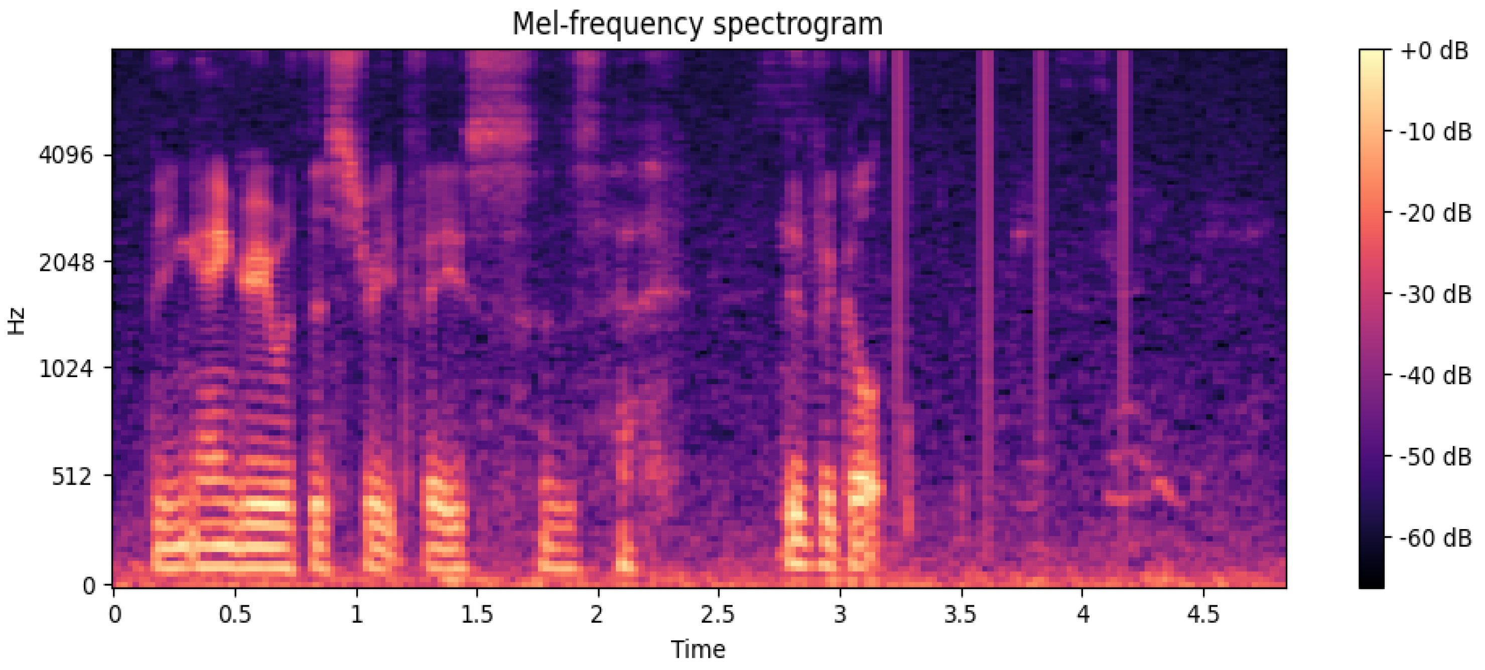
Figure 4 presents the Mel-frequency spectrogram of a sample from the MSP-IMPROV database. Similar to IEMOCAP, the spectrogram illustrates the energy distribution across different frequency bands over time, highlighting the acoustic properties used for emotion recognition.

3.2. Experimental Configuration and Evaluation Metrics

All experiments were conducted on a machine equipped with NVIDIA Quadro RTX 6000 GPUs, running CUDA 12.4 and NVIDIA driver version 550.54.14. This configuration supports accelerated computation for both the training and inference phases of our models.

In order to mitigate the risk of overfitting, a range of techniques were employed. In particular, the AdamW optimizer was employed with a weight decay of 1 $\times {10}^{-4}$ for the purpose of regularization. A ReduceLROnPlateau scheduler, with a factor of 0.1 and a patience of 10, was employed to dynamically adjust the learning rate. Dropout layers with a rate of 0.6 were integrated into the classifier to randomly deactivate neurons during training. Furthermore, pooling layers within the graph convolution layers facilitated the aggregation of node information, thereby reducing complexity and dimensionality. To further stabilize training and prevent overfitting, batch normalization layers were applied after the classifier’s linear layers, which normalized inputs and reduced internal covariate shift.

We employed five-fold cross-validation to assess the performance of our model. The dataset was randomly partitioned into five equal parts, with one serving as the validation set, and the other four parts were used for model training. This iterative process ensures that every subset is tested exactly once, providing a comprehensive and robust evaluation of the generalization ability of the model. This method helps minimize bias and variance, offering a more reliable measure of performance using the full dataset across multiple training scenarios.

To evaluate the performance of the model comprehensively, we employed two metrics: weighted accuracy (WA) and unweighted accuracy (UA). These metrics were selected to capture the model’s performance for both imbalanced and balanced class distributions.

The weighted accuracy accounts for the number of samples in each class, providing a more accurate representation of the performance of the model on an imbalanced dataset. The formula for WA is

$$\mathrm{WA}={\displaystyle \frac{{\sum }_{i=1}^{N}T{P}_i}{{\sum }_{i=1}^N(T{P}_i+F{P}_i)}}$$

(20)

where $T{P}_i$ refers to the true positives for class i, $F{P}_i$ refers to the false positives, and N is the total number of classes.

Unweighted accuracy, on the other hand, calculates the accuracy for each class individually and then averages the results. This ensures that all classes are given equal importance, regardless of their sample size. The formula for UA is given by

$$\mathrm{UA}={\displaystyle \frac{1}{N}}\sum _{i=1}^N{\displaystyle \frac{T{P}_i}{T{P}_i+F{P}_i}}$$

(21)

where $T{P}_i$ and $F{P}_i$ again represent the true positives and false positives for each class i, and N is the number of classes. This metric provides a balanced evaluation of the model’s performance across all classes, making it particularly useful in cases of class imbalance.

3.3. Results and Analysis

In our comprehensive experiments, we rigorously evaluated the performance of our proposed method, SkipGCNGAT, by comparing it against several state-of-the-art models in the field. To ensure a thorough assessment, we employed both the WA and UA as our primary evaluation metrics, which allowed us to measure the overall accuracy of each model and its ability to handle class imbalances effectively. This comparison provides a clear insight into how SkipGCNGAT performs in relation to existing approaches, demonstrating its strengths and contributions to the task of speech emotion recognition. The following provides a concise overview of the key methodologies employed for comparison in our study.

The CNN-LSTM-DNN 2019 [42] proposed a speech emotion recognition model that combined a CNN for powerful feature extraction and LSTM for modeling long-term contextual information. CNNs capture emotional features across multiple temporal resolutions, whereas LSTM tracks dynamic changes in emotional expressions. This approach allows effective emotion recognition in speech, achieving a performance comparable to that of models using handcrafted features.

The Compact-SER 2021 [20] method is a novel approach that transforms speech signals into graph structures and uses a GCN for classification, thus breaking away from traditional SER methods that rely on temporal models or CNNs. By leveraging a GCN to extract features from node characteristics and learn the dependencies between nodes, this study achieved precise graph convolution operations, thereby avoiding the performance loss caused by approximate convolution used in traditional GCNs.

The LSTM-GIN 2021 [22] introduces a novel approach that leverages the power of GNNs. This innovative model, named LSTM-GIN, transforms speech signals into a graph-structured representation and utilizes a GIN for effective global emotion modeling in the non-Euclidean space.

The GraphSAGE-equal 2022 [23] method transforms the SER problem into a graph classification task by converting variable-length speech into a graph structure, thereby avoiding padding or clipping operations and better preserving emotional information. For the first time in the SER field, multi-head attention pooling (MHAPool) was used to encode high-order interactions between nodes and focus on emotionally relevant features, thereby extracting emotional information from speech more effectively.

TLGCNN 2024 [24] employs an adaptive adjacency matrix to automatically learn the spatial relationships between nodes based on the characteristics of speech data, making the model more suitable for speech emotion recognition tasks. Simultaneously, it utilizes Bi-LSTM to extract the temporal dependencies of speech features and LGCN to extract spatial dependencies and comprehensively capture speech emotion information.

Based on the performance in

Table 1. Performance comparison of different methods on the IEMOCAP database.

Method	UA (%)	WA (%)
GCN 2017 [19]	52.36	56.14
SegCNN 2019 [8]	62.34	64.53
CNN-LSTM 2019 [42]	59.23	-
CNN-LSTM-DNN 2019 [42]	60.23	-
GA-GRU 2020 [43]	63.80	62.27
Compact-SER 2021 [20]	62.27	65.29
LSTM-GIN 2021 [22]	64.65	65.53
GraphSAGE-equal 2022 [23]	65.43	66.40
TLGCNN 2024 [24]	64.21	66.82
SkipGCNGAT	65.61	67.37

for the IEMOCAP database, SkipGCNGAT shows notable improvements over traditional deep learning models such as SegCNN [8], CNN-LSTM [42], and GA-GRU [43], with enhancements ranging from 1.81% to 6.38%. SkipGCNGAT surpasses the Compact-SER method [20] with a significant margin, achieving an improvement of approximately 3.34% (p < 0.01, the confidence interval is (2.76, 3.92)) in UA and 2.08% (p < 0.001, the confidence interval is (1.42, 2.74)) in WA, respectively, through the integration of GCN and GAT layers for enhanced adaptive feature extraction.

Compared to LSTM-GIN 2021 [22], SkipGCNGAT improves UA by 0.96% and WA by 1.84%. While LSTM-GIN employs LSTM layers combined with GINs for effective global emotion modeling, its lack of attention mechanisms limits its ability to dynamically prioritize critical node interactions. SkipGCNGAT, on the other hand, incorporates GATs, which assign adaptive attention weights to neighboring nodes, allowing for more nuanced and dynamic feature extraction. Additionally, the use of skip connections ensures smoother information flow across layers, further enhancing the ability of the model to capture emotional nuances in speech, whereas LSTM-GIN may be limited by its more static feature modeling approach.

Compared to GraphSAGE-equal [20], SkipGCNGAT improves UA and WA by 0.18% and 0.97%, respectively. The fixed graph structure of GraphSAGE may limit its ability to capture dynamic dependencies, whereas SkipGCNGAT’s cycle graph structure with adaptive skip connections ensures better information retention.

Compared to TLGCNN [24], SkipGCNGAT achieved a 1.4% and 0.55% improvement in UA and WA, respectively. Unlike TLGCNN’s reliance on Bi-LSTM and predefined spatial structures, SkipGCNGAT’s GAT layer dynamically adjusts the importance of relationships, leading to better modeling of long-range dependencies and emotional shifts in speech.

In

Table 2. Performance comparison of different methods on the MSP-IMPROV database.

Method	UA (%)	WA (%)
GCN 2017 [19]	51.42	54.71
CNN-LSTM 2019 [42]	-	52.36
CNN-LSTM-DNN 2019 [42]	-	52.43
Compact-SER 2021 [20]	54.32	56.24
GraphSAGE-equal 2022 [23]	56.83	60.91
TLGCNN 2024 [24]	56.47	58.35
SkipGCNGAT	57.33	58.96

, by comparing the performance of the MSP-IMPROV database, the SkipGCNGAT method continues to yield competitive results. While the WA is slightly lower than GraphSAGE-equal (58.96% vs. 60.91%), SkipGCNGAT achieves a higher UA of 0.50% (57.33% vs. 56.83%). This slight difference in UA suggests that GraphSAGE-equal [20] may have a marginal edge in balancing the performance across all classes.

In addition, SkipGCNGAT demonstrates a statistically significant improvement over the GCN method [19], with an increase of 4.25% in WA (p < 0.001, the confidence interval is (3.50, 4.99)) and 5.91% in UA (p < 0.001, the confidence interval is (4.82, 6.99)), further emphasizing the efficacy of integrating GCN and GAT layers for capturing intricate relationships within speech data. Compared to Compact-SER [20], SkipGCNGAT improves WA by 2.72% and UA by 3.01%, underscoring the advantage of using attention mechanisms to enhance feature extraction.

Moreover, when compared to CNN-LSTM [42] and CNN-LSTM-DNN [42], SkipGCNGAT provided significant gains, with a WA improvement of 6.60% over CNN-LSTM and 6.53% over CNN-LSTM-DNN, further demonstrating its ability to effectively model temporal and spatial dependencies in speech. A comparison with the TLGCNN [24] shows a 0.61% improvement in WA and a 0.86% improvement in UA, demonstrating how the dynamic attention mechanism of SkipGCNGAT enhances its ability to prioritize important node relationships and handle complex emotional shifts.

Overall, SkipGCNGAT demonstrated clear superiority over traditional and current models across both the IEMOCAP and MSP-IMPROV datasets. It consistently achieved higher WA and UA scores, demonstrating the robust handling of class imbalances and improved overall recognition accuracy. The use of GAT and SkipGCN layers is essential for extracting complex relationships and enhancing performance, thereby solidifying SkipGCNGAT as a competitive model in speech emotion recognition.

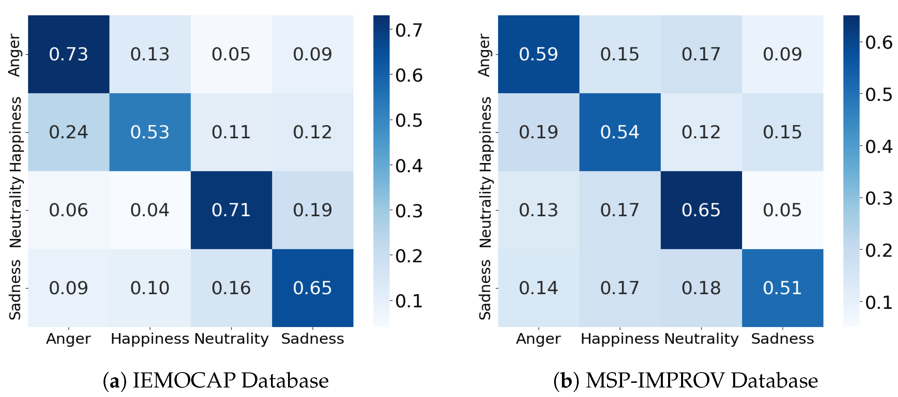
In order to evaluate the performance of our model in classifying emotions, we generated confusion matrices for the IEMOCAP in Figure 5a and MSP-IMPROV datasets in Figure 5b. By visualizing the classification results, the confusion matrices allow us to examine the extent to which the model is able to distinguish between different emotion categories.

The confusion matrices for both the IEMOCAP and MSP-IMPROV datasets highlight the strengths of our model in recognizing key emotional categories. Notably, the model demonstrates a strong ability to accurately classify emotions such as “Anger” and “Neutrality”, with accuracies reaching 73% and 71% on the IEMOCAP dataset, respectively. These results indicate that the model effectively captures distinct emotional features, particularly for emotions with clearer acoustic markers. Furthermore, the performance of model on the MSP-IMPROV dataset remains consistent, particularly with “Neutrality” and “Happiness”, where it shows a reliable classification rate, suggesting that the model generalizes well across different datasets with varied speakers and scenarios. The confusion matrices demonstrate the ability of model to handle complex emotional data while minimizing confusion between closely related emotional states.

3.4. Effect of Different Numbers of SkipGCN Layers

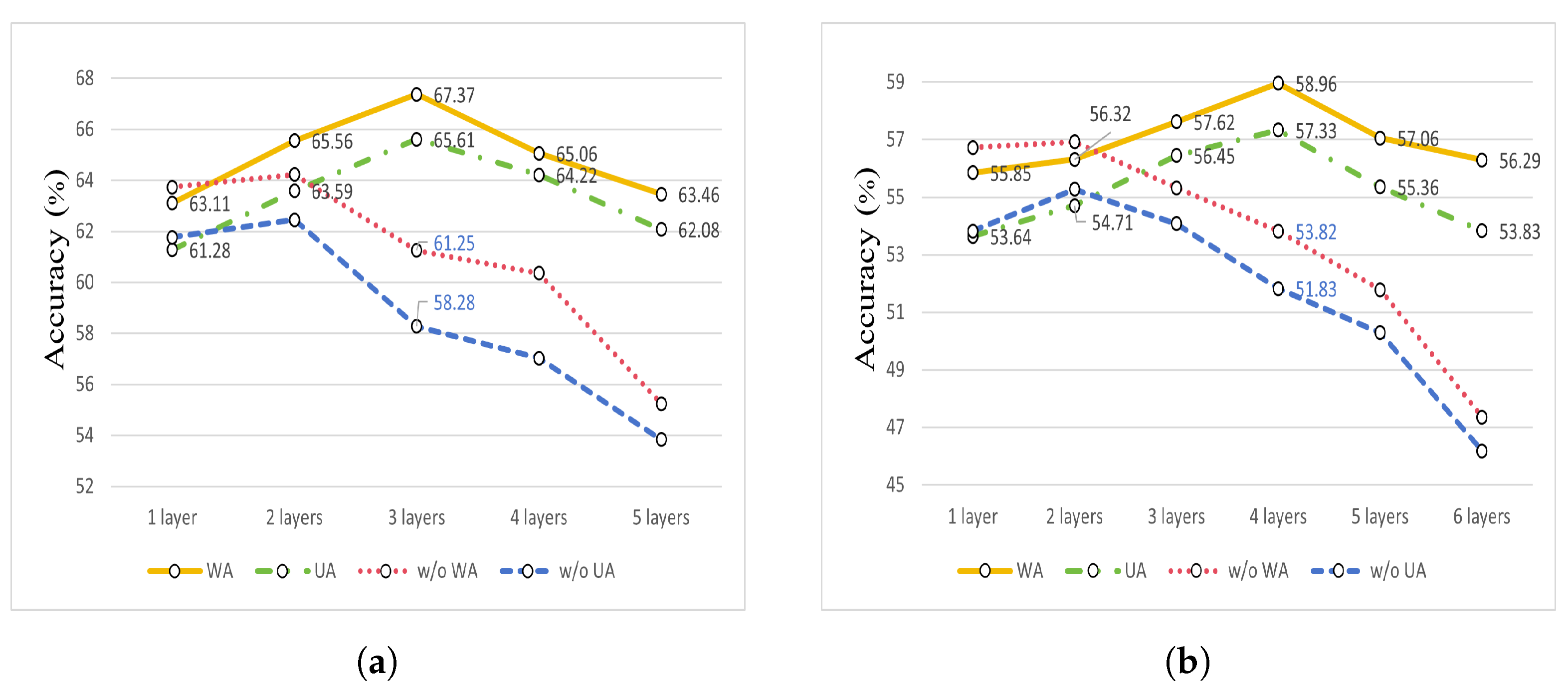
To analyze the impact of different numbers of SkipGCN layers on the WA and UA performance, we conducted experiments on both the IEMOCAP and MSP-IMPROV datasets. By varying the number of SkipGCN layers, we visualized the changes in the WA and UA using line graphs, allowing for a clear and intuitive observation of the trends in model performance as the layer count increased.

In Figure 6, Figure 6a presents the experimental results for the IEMOCAP dataset, and Figure 6b shows the results for the MSP-IMPROV dataset. The solid lines represent the results with skip connections and the dashed lines represent the results without them.

In Figure 6a, the experimental results for the IEMOCAP dataset show that the 3-layer SkipGCN achieves the best performance, with a WA of 67.37% and UA of 65.61%. Compared with the results without skip connections (without WA: 61.25%, without UA: 58.28%), SkipGCN improved the WA and UA by 6.12% and 7.33%, respectively. This significant improvement highlighted the effectiveness of skip connections, with the 3-layer SkipGCN delivering the most substantial boost for this dataset.

In Figure 6b, the results for the MSP-IMPROV dataset reveal that owing to the diversity in scenes and speakers, a 4-layer SkipGCN yields the best performance (WA: 58.96%, UA: 57.33%). The differences compared to the model without skip connections (w/o WA: 53.82%, w/o UA: 51.83%) were 5.14% for WA and 5.5% for UA. Thus, the 4-layer SkipGCN configuration was selected as optimal for the MSP-IMPROV dataset.

Additionally, the results indicated that when using only one layer on the IEMOCAP dataset and the first two layers on the MSP-IMPROV dataset, the models without skip connections outperformed those with skip connections. This suggests that skip connections provide minimal benefits when the model has fewer layers because the depth of model is insufficient to suffer significantly from vanishing gradients or from overfitting issues. With fewer layers, simpler structures can learn the relationships within the data effectively without requiring skip connections. However, as the model depth increases, skip connections become increasingly crucial, allowing the model to better leverage deeper architectures, improve information flow, and mitigate degradation issues, particularly when handling more complex data representations as seen in deeper layers. These observations emphasize that the effectiveness of skip connections is highly dependent on the model depth and the complexity of the dataset.

3.5. Computational Complexity

In order to gain a comprehensive understanding of the performance and resource requirements of the SkipGCN model across different layer depths, a detailed analysis of computational complexity was conducted. Specifically, the SkipGCN model was assessed with 1 to 6 layers on two datasets—IEMOCAP and MSP-IMPROV—focusing on the following metrics: floating-point operations (FLOPs, in millions, as a measure of computational workload), the number of parameters (Param, in millions, indicating the size of the model), and runtime memory usage (Memory, in megabytes, reflecting the memory footprint during execution). These metrics are crucial for evaluating the efficiency of the model, especially in scenarios where computational resources are limited.

Table 3. The computational complexity under different layers of SkipGCN.

	IEMOCAP			MSP-IMPROV
Number of SkipGCN Layers	FLOPs (M)	Param (M)	Memory (MB)	FLOPs (M)	Param (M)	Memory (MB)
1 layer	0.1606	0.1978	0.83	0.1603	0.1976	0.82
2 layers	0.1606	0.1978	0.83	0.1603	0.1976	0.82
3 layers	0.1606	0.1978	0.83	0.1603	0.1976	0.82
4 layers	0.1934	0.2315	0.96	0.1931	0.2313	0.96
5 layers	0.2261	0.2652	1.09	0.2259	0.2649	1.09
6 layers	0.2589	0.2988	1.22	0.2586	0.2986	1.22

highlights the relationship between the number of SkipGCN layers and the associated FLOPs, number of parameters, and memory usage. When comparing models with different layers, it is evident that configurations with 1 to 3 SkipGCN layers exhibit stable computational complexity, as both FLOPs and parameters remain constant. This stability arises because these initial layers are optimized and share a similar feature extraction dimension, effectively preventing significant changes in computational demands. However, from the fourth layer onward, the FLOPs, number of parameters, and memory usage gradually increase. This increase occurs because, at this point, more features and interactions are introduced, requiring more complex transformations and additional computational resources. The addition of each new layer contributes to more parameters being learned, which, in turn, increases memory usage and computational cost.

The results indicate that adding more layers leads to a moderate increase in computational overhead. However, this incremental increase remains controlled, demonstrating that architecture of our model scales efficiently with the number of layers. The steady growth in parameters and FLOPs reflects the capacity of model to capture increasingly complex patterns and interactions without drastically increasing computational burden.

For the IEMOCAP dataset, we ultimately selected the 3-layer SkipGCN configuration based on accuracy, whereas for the MSP-IMPROV dataset, the 4-layer SkipGCN configuration was found to be optimal. Subsequently, we conducted additional experiments with varying numbers of GAT heads to provide a more comprehensive analysis of computational complexity, as shown in

Table 4. The computational complexity with varying numbers of GAT heads.

	IEMOCAP			MSP-IMPROV
Number of GAT Heads	FLOPs (M)	Param (M)	Memory (MB)	FLOPs (M)	Param (M)	Memory (MB)
1 head	0.1606	0.1729	0.73	0.1931	0.2065	0.86
2 heads	0.1606	0.1812	0.76	0.1931	0.2149	0.89
3 heads	0.1606	0.1895	0.79	0.1931	0.2232	0.93
4 heads	0.1606	0.1978	0.83	0.1931	0.2313	0.96
5 heads	0.1606	0.2059	0.86	0.1931	0.2396	0.99

.

Table 4 presents the computational complexity of the model with varying numbers of GAT heads. As the number of GAT heads increases, the number of parameters and memory usage also gradually increase, while the FLOPs remain stable. Increasing the number of GAT heads can improve the ability of model to capture complex feature relationships and enhance its feature extraction capability. However, this also results in additional parameter and memory overhead, which requires balancing computational resources and model performance in practical applications. We chose to use four GAT heads primarily to enhance the representational capacity of model while controlling computational complexity, ensuring that the model maintains high efficiency and reasonable resource usage during task processing.

We assess the performance of our model by comparing it to the state-of-the-art deep graph models, using identical node features and a cyclic graph structure. PTCHY-SAN [44] is a graph neural network model that learns convolutional neural networks (CNNs) for arbitrary graphs, focusing on effective graph classification by extracting and standardizing local node neighborhoods in a way similar to image CNNs. PTCHY-Diff [45] is a hierarchical GCN approach with differentiable pooling layers between graph convolution layers to perform hierarchical representation learning, improving the ability to extract features from complex graph structures. BLSTM [46] utilizes a bidirectional long short-term memory network (BLSTM) to encode speech signals and employs the hidden state at the final time step as the context vector for the entire sentence.

The

Table 5. Comparison of the number of parameters of models.

GCN [19]	PTCHY-SAN [44]	PTCHY-Diff [45]	BLSTM [46]	Compact-SER [20]	Ours
∼76 K	∼60 K	∼68 K	∼0.8 M	∼30 K	∼0.2 M

illustrates that our model has approximately 0.2 M parameters, significantly fewer than the BLSTM [46] model, which requires about 0.8 M parameters, indicating a reduction in computational overhead. Although our model has a greater number of parameters than Compact-SER [20], GCN [19], PTCHY-SAN [44], and PTCHY-Diff [45], our model has a thoughtful balance between model complexity and the performance necessary for accurate emotional recognition. The parameter count of our model ensures good performance without the burden of an excessively large model. However, there is potential for further refinement of our model, aiming to decrease its size while preserving or even enhancing its recognition capabilities, which is particularly relevant for applications with constrained computational resources.

3.6. Ablation Studies

In this section, we discuss the effectiveness of two key components of the SkipGCNGAT model, the GAT module and the proposed architecture, which combines the outputs of the two SkipGCN modules before applying pooling. Through ablation experiments, we analyzed the impact of removing or modifying these components, thereby highlighting their contribution to the overall performance of our model. The results of these experiments demonstrate the importance of the attention mechanism of the GAT module in prioritizing crucial node relationships as well as the advantage of combining outputs from multiple SkipGCN layers to capture both local and global features more comprehensively.

The results in

Table 6. Ablation study on the effectiveness of GAT module in SkipGCNGAT model.

	IEMOCAP		MSP-IMPROV
Method	WA (%)	UA (%)	WA (%)	UA (%)
GAT	67.37	65.61	58.96	57.33
w/o GAT	66.08	64.67	57.84	57.01
2-layer GAT	46.36	43.28	39.46	36.26

demonstrate the effectiveness of the GAT module in enhancing the performance of the SkipGCNGAT model, particularly in terms of the WA on both the IEMOCAP and MSP-IMPROV datasets. When the GAT was included, the model showed significant improvements in WA, highlighting the importance of this component in capturing crucial relationships between nodes in the graph.

For the IEMOCAP dataset, the incorporation of the GAT module resulted in a notable enhancement in performance, increasing WA from 66.08% to 67.37%, representing a substantial gain of 1.29% (p < 0.05, the confidence interval is (0.81, 1.77)), and UA from 64.67% to 65.61%, with an increase of 0.94% (p < 0.001, the confidence interval is (0.42, 1.46)). This improvement reflects how the attention mechanism allows the model to focus on more important nodes and edges, improving the overall classification accuracy. Although the UA also improves, the increase is less pronounced, indicating that GAT significantly affects the overall performance of the model more than on balancing the class-specific accuracy.

On the MSP-IMPROV dataset, the GAT module once more demonstrated its utility, yielding an improvement in WA by 1.12% (from 57.84% to 58.96%), with a confidence interval of (0.68, 1.56) at a significance level of p < 0.05, and an increase in UA by 0.32% (from 57.01% to 57.33%), with a confidence interval of (0.18, 0.46) at a significance level of p < 0.001. This dataset, characterized by diverse speakers and environments, benefits from the dynamic attention mechanism in GAT, which helps the model focus on the most informative relationships between speech frames. Here, improvements in both WA and UA demonstrate that the GAT is particularly effective in addressing class imbalances in more complex datasets.

The addition of a 2-layer GAT, as presented in Table 6, results in a noticeable performance drop compared to the single-layer GAT. Our model uses multi-head attention with four heads, and adding another GAT layer substantially increases the number of parameters. This rapid growth in complexity leads to overfitting, causing the model to fit too closely to the training data, which reduces its ability to generalize to new data. Consequently, a single-layer GAT with four attention heads is more effective, providing a good balance between capturing critical relationships and maintaining generalizability without overwhelming the model with excessive parameters.

Table 7. Ablation study on the effectiveness of pre-pooling SkipGCN combination in SkipGCNGAT model.

	IEMOCAP		MSP-IMPROV
Method	WA (%)	UA (%)	WA (%)	UA (%)
Pre-Pooling SkipGCN Combination	67.37	65.61	58.96	57.33
w/o Combination	66.12	64.21	57.35	56.47

presents the results of an ablation study that focuses on the effectiveness of combining the two SkipGCN modules before pooling, specifically within the SkipGCNGAT model. In this architecture, each SkipGCN module consists of multiple layers, and the outputs of the two blocks are combined before the final pooling and classification stages. The performance of this configuration was evaluated on both the IEMOCAP and MSP-IMPROV datasets.

The results show that the pre-pooling combination of SkipGCN modules contributed positively to the overall model performance on both datasets. For the IEMOCAP dataset, the integration of SkipGCN modules prior to pooling showed a statistically significant enhancement in performance, with an increase of 1.25% in WA (p < 0.05, the confidence interval is (0.72, 1.78)) and 1.40% in UA (p < 0.01, the confidence interval is (0.89, 1.91)), underscoring the benefits of combining SkipGCN layers for improved feature extraction and emotion recognition. This improvement suggests that combining the outputs of SkipGCN layers before pooling enhances the ability of the model to integrate diverse feature representations more effectively, leading to improved overall performance.

Similarly, on the MSP-IMPROV dataset, the combination of SkipGCN modules yielded an increase of 1.61% in WA (p < 0.05, the confidence interval is (0.85, 2.37)) and 0.86% in UA (p < 0.1, the confidence interval is (0.21, 1.51)). These results highlight that the combination of multiple SkipGCN layers enriches the spatiotemporal feature representation, leading to better classification accuracy.

4. Conclusions

In this study, we propose SkipGCNGAT, a novel hybrid model that integrates SkipGCN and GAT for speech emotion recognition. Through comprehensive experiments on two benchmark datasets, IEMOCAP and MSP-IMPROV, our method demonstrates significant improvements in both the WA and UA compared with several state-of-the-art models.

One of the key findings was the effectiveness of incorporating skip connections in the SkipGCN layers, which consistently improved model performance, particularly when using deeper networks with more layers. The attention mechanism provided by the GAT further enhanced the ability of the model to prioritize critical node relationships, leading to a noticeable increase in overall accuracy. Our ablation experiments confirmed that both the GAT module and the combination of multiple SkipGCN layers before pooling were essential components contributing to the robustness and effectiveness of the model.

Moreover, our model achieved superior results on the IEMOCAP dataset with 67.37% WA and 65.61% UA, as well as competitive performance on the MSP-IMPROV dataset, where it delivered a WA of 58.96% and a UA of 57.33%. These results highlight the importance of capturing both local and global dependencies in speech data and demonstrate the potential of SkipGCNGAT for improving emotion recognition tasks.

The SkipGCNGAT model holds the promise of substantially enhancing user experiences across a range of applications, including virtual assistants, call centers, and emotional AI systems. By facilitating more precise and sophisticated emotion detection, our model paves the way for interactions that are not only more responsive but also deeply attuned to the user’s emotional state, thereby fostering a more empathetic and personalized engagement. Moving forward, we aim to investigate the application of this framework in other domains where the understanding of spatial–temporal dynamics is pivotal. Additionally, we plan to refine the skip connection and attention mechanisms to further bolster the model’s performance across diverse datasets, thereby broadening its real-world utility and impact.