Article

Task-Level Customized Pruning for Image Classification on Edge Devices †

by
Yanting Wang
1,2,*,
Feng Li
1,
Han Zhang
3 and
Bojie Shi
1
1
School of Software, Northwestern Polytechnical University, Xi’an 710072, China
2
Research & Development Institute of Northwestern Polytechnical University in Shenzhen, Shenzhen 518057, China
3
China Unicom Research Institute, Beijing 100085, China
*
Author to whom correspondence should be addressed.
This paper is an extended version of our paper published in Wang, Y.; Li, F.; Zhang, H. TA2P: Task-Aware Adaptive Pruning Method for Image Classification on Edge Devices. In Proceedings of the ICASSP 2024—2024 IEEE International Conference on Acoustics, Speech and Signal Processing (ICASSP), Seoul, Republic of Korea, 14–19 April 2024.
Electronics 2024, 13(20), 4029; https://doi.org/10.3390/electronics13204029
Submission received: 28 August 2024 / Revised: 2 October 2024 / Accepted: 11 October 2024 / Published: 13 October 2024
(This article belongs to the Section Artificial Intelligence)

Abstract

:
Convolutional neural networks (CNNs) are widely utilized in image classification. Nevertheless, CNNs typically require substantial computational resources, posing challenges for deployment on resource-constrained edge devices and limiting the spread of AI-driven applications. While various pruning approaches have been proposed to mitigate this issue, they often overlook a critical fact that edge devices are typically tasked with handling only a subset of classes rather than the entire set. Moreover, the specific combinations of subcategories that each device must discern vary, highlighting the need for fine-grained task-specific adjustments. Unfortunately, these oversights result in pruned models that still contain unnecessary category redundancies, thereby impeding the potential for further model optimization and lightweight design. To bridge this gap, we propose a task-level customized pruning (TLCP) method via utilizing task-level information, i.e., class combination information relevant to edge devices. Specifically, TLCP first introduces channel control gates to assess the importance of each convolutional channel for individual classes. These class-level control gates are then aggregated through linear combinations, resulting in a pruned model customized to the specific tasks of edge devices. Experiments on various customized tasks demonstrate that TLCP can significantly reduce the number of parameters, by up to 33.9% on CIFAR-10 and 14.0% on CIFAR-100, compared to other baseline methods, while maintaining almost the same inference accuracy.

1. Introduction

With the explosive growth of intelligent applications on edge devices in recent years, convolutional neural networks (CNNs), as the mainstream deep learning model architecture, have been widely adopted in various visual tasks, such as image classification, object detection, and image segmentation [1,2,3]. As these visual tasks grow increasingly complex, numerous CNN architectures, such as AlexNet [4], VGGNet [5], ResNet [6], and DenseNet [7], have been proposed to enhance performance. However, this success is accompanied by the challenge of an escalating number of model parameters, which leads to a significant increase in multiply–accumulate (MAC) and floating-point operations (FLOPs). These increases directly conflict with the inherent limited resources of edge devices.
To reduce the number of parameters and computational cost of CNNs, various model compression methods have been proposed, such as weight quantization [8,9], low-rank matrix decomposition [10,11], tensor decomposition [12,13,14,15,16], and pruning [17,18,19,20,21,22,23,24,25,26]. Among them, model pruning is more popular since it offers superior compression performance. Generally, it can be categorized into non-structured pruning [17,18,19] and structured pruning [20,21,22,23,24]. Non-structured pruning refers to assessing parameter importance and selectively eliminating certain weights and neurons. This method facilitates higher flexibility. In addition, the generated sparse matrix can also be used for further model optimization and compression. However, specialized hardware and libraries are required to achieve efficient computation and compression of sparse matrices, which in turn limits the scope of application for non-structured pruning [27]. On the contrary, structured pruning involves organized pruning of a certain structure of the neural network, such as filters, channels, or layers, while retaining the original convolution structure [24]. Hence, it does not require dedicated hardware to be implemented. With standard hardware, improved acceleration and compression can be achieved by leveraging highly efficient libraries, such as the Basic Linear Algebra Subprograms (BLAS) library. As a result, it is more suitable for scenarios where hardware friendliness and computational effectiveness are of greater demand. Moreover, the significance of this approach is particularly notable given the trend towards deeper neural networks [28].
Although these pruning methods can effectively reduce model parameters and computational cost, there are still deficiencies. Firstly, these pruning methods overlook differences in fine-grained task information, leading to category redundancy at the task level in the pruning result. More specifically, these existing pruning schemes typically assume that the device needs to classify all classes within a dataset. However, in real-world scenarios [29,30], devices often only need to focus on certain combinations of subcategories, not all categories. Moreover, different devices pay attention to varying combinations of subcategories, which we refer to as differences in fine-grained task information. According to experimental verification by our previous work [31], making rational use of this fine-grained task information could further improve flexibility of model pruning, and thus, make the pruned model more lightweight. However, the challenge of how to incorporate fine-grained task information into the pruning process remains to be fully explored. Secondly, the operations of deleting or retaining neural network weights/connections in the aforementioned pruning operations lack clear explanatory rationale, leading to a decrease in the credibility of model decision behavior. In practical applications, especially in critical fields such as medicine, finance, and security, the model decision-making process needs to be transparent to ensure the credibility and normalization of model behavior. Based on the above, it is urgent to carry out this research to explore how to ensure interpretability of the pruning process while considering differences in fine-grained task information.
To this end, this work proposes a task-level customized pruning method. The core concept behind TLCP rests on the observation that neurons/filters contribute unequally to the classification of images from different classes, since images of different classes activate unique neuron pathways across network layers [32,33]. As illustrated in Figure 1, green neurons are crucial for classifying the “goldfish” category because they are strategically located within neural pathways specifically associated with that category. Conversely, the key pathway for the “cat” category is very different from that of the “goldfish” category, with completely different critical neurons within the same layer. In the proposed method, we utilize channel control gates to quantify the contribution of each convolutional channel during the model’s forward propagation, forming image-level, class-level, and task-level control gates successively. Specifically, we first associate a control gate with each individual output channel of a layer for a single image input, which enables image-level mapping of channel contributions. Since each image contributes equally to the class, we fuse image-level control gates of the same label via simply adding them together, and thus, obtain the class-level control gate. As mentioned earlier, one task is composed of various classes. In addition, different tasks involve different class combinations. To tailor customized control gates for each task, we propose fusing class-level control gates of targeted classes. Since various classes contribute differently, we adopt the linear combination approach with weights denoting their difference. Here, weights for each class are optimized via two methods, i.e., Particle Swarm Optimization (PSO) and Genetic Algorithm (GA) iterative processes. Based on this obtained customized control gate, we finally achieve a task-aware pruned model. Extensive simulations verify the high effectiveness of the proposed method, especially when the number of classes within one task is small.
The main contributions of this paper are as follows:
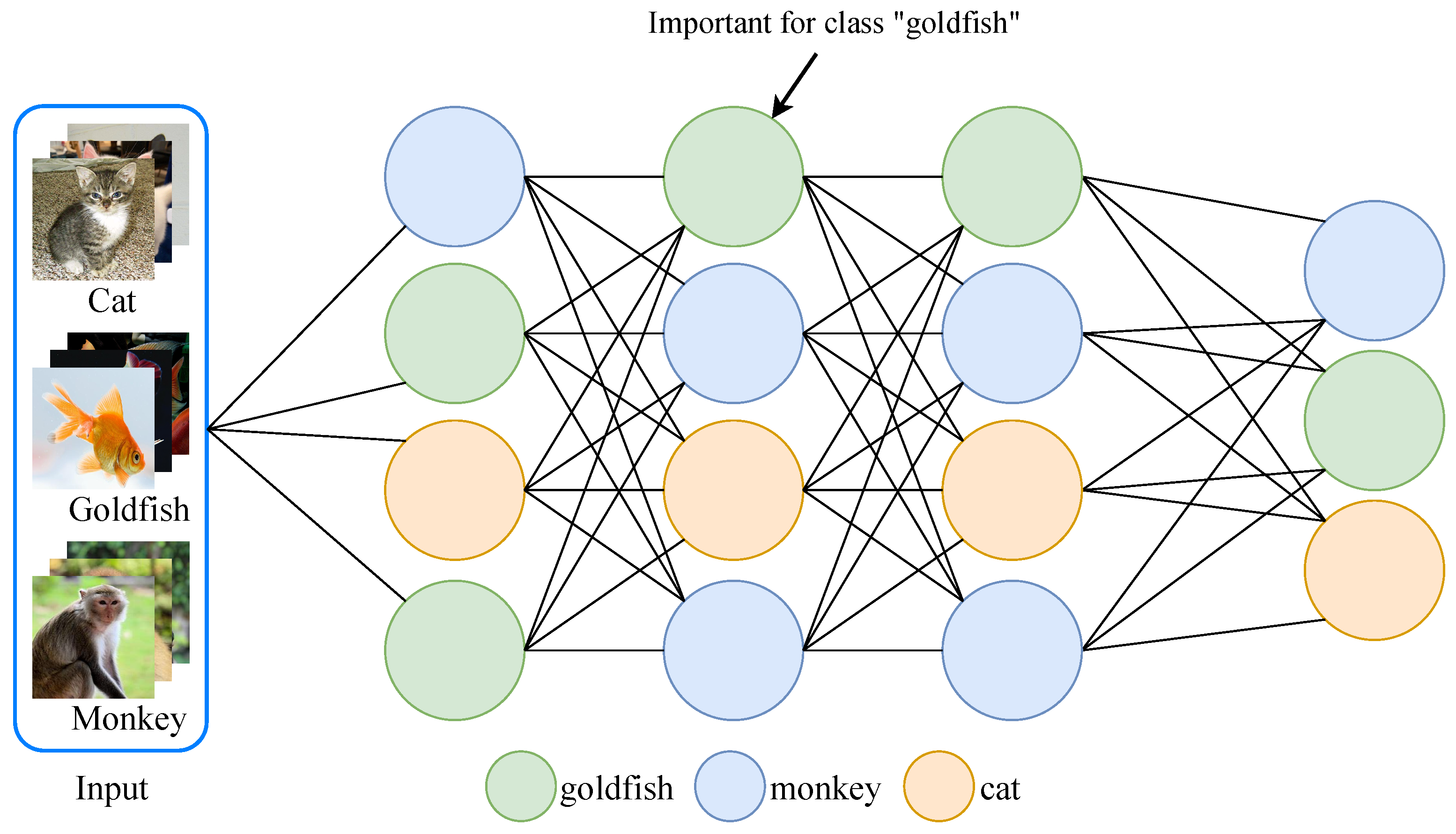
  • Observing that edge-side tasks only need to process a subset of classes, we propose a customized pruning method based on the fine-grained information of task, which also conforms to the development trend of wisdom sinking.
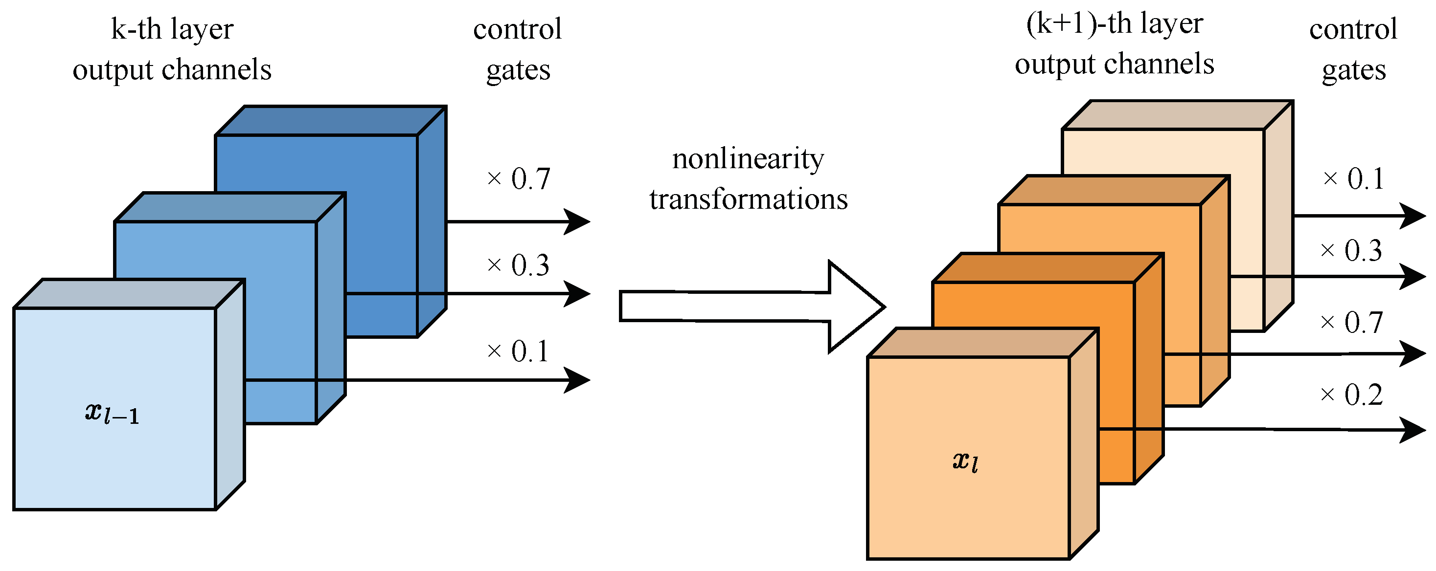
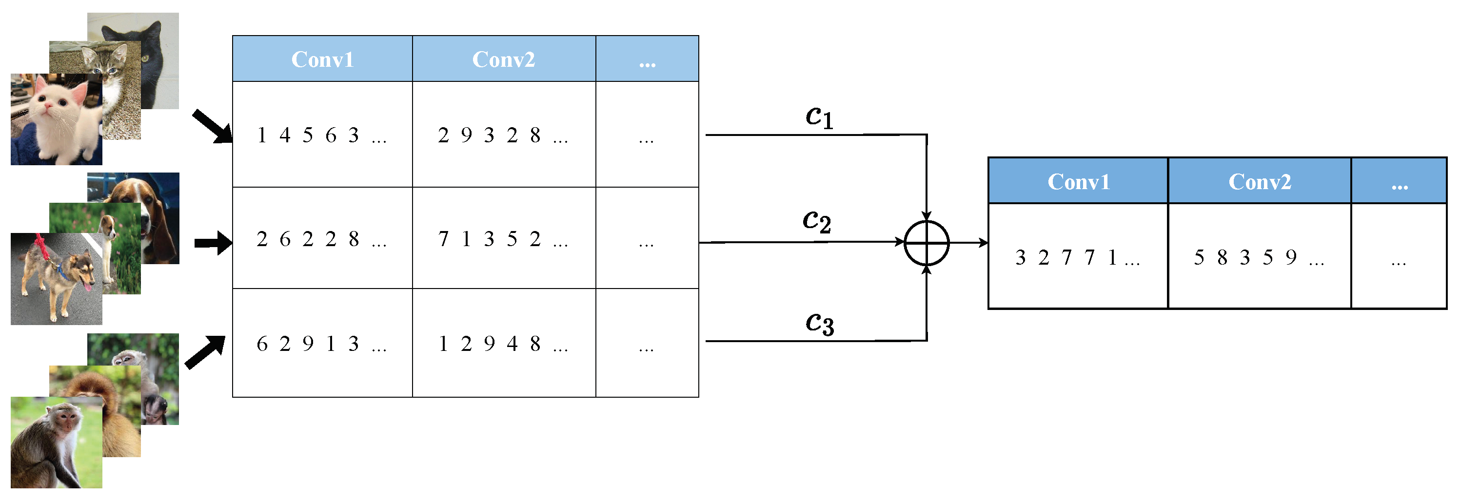
  • In this method, we utilize channel-wise control gates to quantify individual channel contributions. Via processing these control gates, e.g., linear combination among different classes, a customized lightweight network is realized.
  • Experimental results on three datasets demonstrate the proposed method can significantly decrease the number of network parameters while maintaining nearly identical performance compared to baselines.
The rest of this paper is organized as follows. Section 2 presents the related work. Section 3 gives details of the proposed method; this is followed by experiments and analysis conducted on three datasets in Section 4. Finally, a discussion of the algorithm’s implementation and conclusions are provided in Section 5 and Section 6, respectively.

2. Related Work

To better deploy real-time intelligent applications on edge devices, model compression is crucial via lightening advanced deep neural networks (DNNs) with high memory and computation demands. Currently, typical techniques for model compression include tensor decomposition, quantization, low-rank decomposition, and pruning [34].

2.1. Tensor Decomposition

Tensor operations are fundamental computations within neural networks. Consequently, tensor compression emerges as a promising approach to reduce model size and enhance computational effectiveness. Common tensor decomposition methods include canonical polyadic decomposition (CPD) [12], Tucker decomposition (TD) [13,14], and singular value truncation decomposition (SVD) [15,16]. Specifically, CPD extracts hidden structures and features from tensors by decomposing them into outer products. Ref. [12] proposes a dynamic rank reduction (RR) scheme, which explicitly constrains DNN models within a low-rank space during model training to minimize ranks of model weight tensors. Building on this idea, an improved TD method is proposed in Ref. [13], which employs an improved GA to optimize Tucker ranks. Similarly, Gabor. M. et al. propose a novel CNN compression technique based on hierarchical Tucker-2 (HT-2) tensor decomposition in [14]. Derived from SVD, singular value truncation decomposition retains primary singular values and their corresponding vectors to achieve a low-rank approximation of tensors. For instance, LightFormer proposed in [15] utilizes low-rank factorization initialized by SVD-based weight transfer and parameter sharing. Furthermore, Ref. [16] designed a tensor train–tensor singular value decomposition (TT-TSVD) algorithm to preserve the association relationship among tensor singular value decomposition retention modes.
In conclusion, these tensor decomposition methods significantly reduce the number of parameters within models, and thus, lower storage and computational costs. However, this advantage comes at the cost of substantial computational overhead and potential loss of information. It is worth noting that, due to these drawbacks, such methods may be less suitable for edge scenarios, where computational resources and memory constraints are particularly critical.

2.2. Quantization

The core idea of quantization is to reduce memory usage and inference time of the neural network by reducing the bit width of data flowing through the neural network model, thus making it possible to deploy large-scale DNNs on resource-constrained devices. However, quantifying all layers uniformly with ultralow-precision bits often leads to significant performance degradation. To address this, several strategies have been proposed to achieve flexible combinations of different bit widths. For instance, QBitOpt, proposed in [8], formulates the bit-width allocation problem as a constraint optimization problem. Via leveraging fast-to-compute sensitivities and efficient solvers during quantization-aware training (QAT), QBitOpt can produce mixed-precision networks to maintain high task performance while adhering to stringent resource constraints. Similarly, Ref. [9] employs a novel sensitivity metric to allocate the number of bits for each layer efficiently, tailored to a given model size. These bit-width allocation techniques contribute significantly, enhancing their effectiveness across various hardware platforms.
However, quantization also introduces challenges. Due to the reduced bit width of network parameters, some information may be lost, which potentially leads to a decrease in inference accuracy. Moreover, many existing training methods and hardware platforms may no longer be applicable for specific bit widths, necessitating the design of specialized system architectures.

2.3. Low-Rank Decomposition

Convolutional and fully connected layers in neural networks are often overparameterized, which means that their weights lie within a low-rank subspace. Hence, it is possible to represent them with low-rank tensor or with tensor network formats. A hybrid model compression (HMC) method based on sensitivity grouping is proposed in [10], which combines low-rank tensor decomposition with structured pruning. Although low-rank methods can preserve the accuracy of the original model, they may compromise the model’s robustness against adversarial perturbations. To address this issue, a robust low-rank training algorithm is proposed in [11], which maintains networks’ weights within the low-rank matrix manifold while simultaneously enforcing approximate orthonormal constraints. The results demonstrate that the proposed technique significantly reduces memory demand and computational cost during training, while also maintaining or even improving both the accuracy and robustness of the original model.
Although matrix decomposition has made great progress, it still has shortcomings. First, matrix decomposition operations entail high costs, considering that substantial retraining is necessary to achieve model convergence. Additionally, layer-wise decomposition impedes global parameter compression. Moreover, the growing prevalence of 1 × 1 convolutions in recent network architectures poses hurdles for traditional low-rank decomposition methods, complicating network compression and acceleration endeavors.

2.4. Pruning

In the field of model compression, pruning techniques hold a significant position. Pruning involves the removal of redundant or less important weights and neurons from a neural network, effectively reducing its size and complexity without significantly compromising its performance. Generally, pruning techniques can be further divided into unstructured pruning and structured pruning.

2.4.1. Unstructured Pruning

The computational effectiveness of convolutional neural networks (CNNs) can be enhanced through non-structured pruning, which involves the removal of connections with minimal contributions across different layers. The concept of pruning was first introduced in [35], which proposed saliency as a measure of the importance of each weight. Here, saliency is calculated by the diagonal elements of the Hessian matrix. Subsequently, Han et al. suggested an iterative pruning approach using 1 regularization and retraining in [36]. This iterative process gradually prunes weights to achieve resource savings while preserving model accuracy. Recent advancements in non-structured pruning emphasize a deeper integration with hardware acceleration. Ref. [19] enhances effectiveness on GPU platforms by employing a direct sparse algorithm, achieving high sparsity levels without sacrificing accuracy. Moreover, it presents sparse CNN-based architectures with reduced precision, offering superior effectiveness compared to conventional CuDNN libraries. Note that traditional methods often design the model architecture and hyperparameters before training, which leads to neural redundancy. In contrast, Ref. [17] proposes a novel method to prune the neural network structure during training. By removing redundant neurons based on activation values, it effectively compresses and accelerates model parameters.
Although unstructured pruning provides flexibility and high compression rates, it also faces several challenges. For example, operators and hardware adapted to sparsity need to be designed to speed up the calculation, which increases the application cost. Furthermore, parameter-wise pruning incurs computational overhead, which is challenging for edge devices, especially with the trend of deepening model layers.

2.4.2. Structured Pruning

In contrast to unstructured pruning, which employs weight magnitude as the metric, structured pruning utilizes filter norm values as its guiding principle. More specifically, structured pruning removes entire filters from neural networks, and thus, achieves practical acceleration and compression benefits with standard hardware, aided by the utilization of efficient libraries such as BLAS.
One notable approach within structured pruning is to measure the contribution of each channel to facilitate the pruning process. A paradigmatic instance of this methodology is differentiable network channel pruning (DNCP) [20]. DNCP stands out for its efficacy in identifying optimal network configurations that align with predefined resource constraints, such as the number of floating-point operations (FLOPs), by employing a gradient descent optimization strategy. In the DNCP framework, a distinct learnable probability is assigned to the potential channel count in each layer of the network. These probabilities are then fine-tuned in an end-to-end manner through the iterative process of gradient descent. The pruning operation is subsequently executed contingent upon these optimized probabilities, culminating in the emergence of a network substructure that is both efficient and optimal.
Cascade structured pruning (CSP), introduced by [22], is designed to enhance energy efficiency by preserving data reuse opportunities. It induces a predictable sparsity pattern, facilitating low-overhead compression of weight data and sequential access to both activation and weight data. To address limitations of 1-norm regularization in exploiting mobile parallelism while maintaining high inference accuracy, a novel block-based pruning framework is proposed in [23]. This framework leverages reweighted regularization methods to achieve better weight regularization effects in shorter training times. Consequently, it ensures flexibility and real-time mobile acceleration across both CNNs and RNNs. In contrast to static pruning approaches, Ref. [24] presents an automated approach for identifying effective pruned models within predefined computational overhead constraints. This method utilizes differentiable annealing indicators search techniques and various regularizations based on prior structural knowledge to control pruning sparsity and enhance model performance. In more complex networks, structured pruning can also account for dependencies among groups of parameters, such as filters in consecutive layers. Grouped parameter pruning acknowledges the interdependencies within the network structure, a concept that has been explored in earlier studies on structural pruning [37,38]. However, existing techniques largely depend on empirical rules or predefined architectural patterns, which limits their adaptability across diverse network architectures. To overcome this limitation, recent work [39] proposes a more general approach that introduces a dependency graph (DepGraph) that models interdependencies between layers. This framework allows for simultaneous pruning of grouped layers, ensuring that parameters deemed unimportant can be safely removed with minimal performance loss, thus enhancing the versatility of structural pruning across various network architectures.
However, the above pruning methods overlook differences in fine-grained task information, resulting in the inflexibility of the pruning process and incomplete pruning results. Moreover, the deleting operations in the above pruning methods lack clear explanation logic, leading to a decrease in the credibility of model decision behavior. To handle the above issues, this paper proposes a task-level customized pruning method, which can ensure interpretability of the pruning process while considering differences in fine-grained task information.

3. Methods

In this section, we present our proposed method. As shown in Figure 2, TLCP begins with training of image-level channel control gates, which maps the contribution of each channel of the CNN to a channel control gate for a single input/image. After deriving image-level control gates, we merge all gates corresponding to inputs with the same label, obtaining class-level control gates, as described in Section 3.1. Subsequently, to map task information into the network architecture, we fuse targeted class-level control gates to form a customized task-level control gate. Section 3.2 presents the fusion method of linear combination, which uses PSO/GA to iteratively explore weights. This customized control gate effectively reflects the contribution of each convolutional channel under a specified task. Channels with a low gate value are removed after fusion of class-level control gates, thereby generating a customized pruned model tailored to the specific task.

3.1. Class-Level Channel Control Gates

This subsection provides a detailed explanation of how to form a class-level channel control gate, which maps class information to the network structure. Put simply, we utilize control gates to evaluate the importance scores of channels based on their contribution to a targeted class. Additionally, we train control gates for each individual image input, and subsequently, merge these control gates within the same category to generate class-level control gates.
Throughout the model’s forward propagation, different convolutional channels have different levels of contribution for a single input [32,33]. To this end, we introduce control gates with a scalar λ associated with each layer’s output channel to quantify the contributions of different channels. These channel-wise scalars are designed to maximize a neuron’s activation. As shown in Figure 3, a set of control gates λ k is multiplied by the k-th layer’s output channel-wise during the inference forward pass, with dimensions of λ k aligning with the number of convolutional channels in the k-th layer. With the concept of control gates, the model structure can be mapped to A = { λ 1 , λ 2 ,…, λ K }, with K denoting the model’s depth to a certain extent.
To enable control gates to accurately reflect the contribution of each convolutional channel, each λ k should satisfy the following two conditions:
(1) λ k should be non-negative, considering it should only suppress or amplify the activation of the output channel. A negative value would negate the original output activations, leading to significant changes in the activation distribution and introducing unexpected influences during model inference.
(2) λ k should be as sparse as possible, meaning that most of its elements are close to zero. Sparse control gates enhance the emphasis on channel structures with higher contributions while suppressing those with low contributions.
To effectively enable the control gate to reflect the contribution of each channel under an input image x, we transfer the structure of the original model to control gate space, inspired by the knowledge distillation technique [40]. Mathematically, we formulate this problem as follows:
min A L o s s = c r o s s E n t r o p y ( f θ ( x ) , f θ ( x , A ) ) + γ k | λ k | s . t . λ k 0 , k = 1 , 2 , , K ,
where f θ ( x ) and f θ ( x , A ) denote the original full model prediction probability [ p 1 , p 2 , p 3 p m ] and new prediction probability [ q 1 , q 2 , q 3 q m ] , respectively. Here, m is the category number, and γ is a balanced parameter.
Here, we use the gradient descent method to solve this problem. Specifically, the gradients of the control gates can be calculated as
L o s s A = c r o s s E n t r o p y ( f θ ( x ) , f θ ( x , A ) ) A + γ s i g n ( A ) .
After calculating the prediction probability of the original model for a given input, we use Equation (2) to update the control gates. Consequently, for a single input x i , we can derive an optimal control gate A i * , named as an image-level control gate.
Figure 4 shows the comparison of control gate values across all convolutional channels in the 3rd and 7th convolutional layer of VGG-16 on CIFAR-10. Here, Figure 4a,b illustrate the control gate values of each convolutional channel under different labeled inputs, while Figure 4c,d illustrate the control gate values of each convolutional channel for the same labeled image input. For each class, we compute the sum of gate values for each convolutional filter across 100 images. From Figure 4, we can observe that each class is primarily associated with sparse and specific convolutional filters (bright color), while most convolutional channels exhibit little correlation (dark color). For each image within the same label, the convolutional channels with high correlation are almost identical to the statistically high-correlation filters in each layer of the model. In summary, each class is only correlated with sparse and specific filters in the CNN classifier. This observation aligns with the findings of previous works, as referenced in [41,42]. Inputs of the same class usually activate a unique set of neurons, which differ from those activated by other classes and may even be mutually exclusive. The above discovery provides the foundational support for the subsequent analysis and class-level control gate generation. We propose that all image-level control gates of the same class can be merged to obtain class-level control gate, which can reflect class-level information to a certain extent. The class-level control gate of class v Y v can be calculated as
Y v = i A i * .

3.2. Class-Level Control Gate Fusion

Given that convolutional channels activated by inputs from different classes vary, the corresponding control gates Y v also exhibit significant differences. Therefore, we propose a coefficient for each Y v and adopt a linear fusion model to merge different class-level control gates. Mathematically,
Y fusion = v = 1 V c v Y v
with C = [ c 1 , c 2 , , c V ] denoting the weights of the linear combination of V targeted classes. For ease of understanding, we provide a three-class fusion illustration in Figure 5, demonstrating how the customized control gate tailored for a specific task is generated by linearly combining different class-level control gates.
Obviously, different choices of C lead to different task-level control gates, thereby reflecting distinct pruned models. Therefore, the problem of finding a well-performing pruning model for targeted classes reduces to optimizing C. For optimizing parameter C, gradient descent is a commonly utilized method in optimization problems. Typically, this involves calculating the loss function, and subsequently, determining the gradient with respect to C. However, although the chain rule can be used to compute this gradient, formulating a direct loss function for the gradient of C might not be practical when the optimization goal is to minimize the accuracy loss of the pruned model. Therefore, we employ Particle Swarm Optimization (PSO) [43] and Genetic Algorithm (GA) [44] to explore C iteratively.

3.2.1. PSO-Based Control Gate Fusion

In this approach, each particle in PSO is conceptualized as a vector of weights, denoted as [ c 1 , c 2 , , c V ] . These weights define the particle’s position within the solution space, where each weight corresponds to a specific class-level control gate. Essentially, we treat each particle as a candidate solution, and the configuration of its weights represents a potential solution to the problem.Additionally, the particle’s velocity vector indicates the direction and magnitude of its movement for subsequent exploration steps. To evaluate the quality of each particle’s position and guide the iterative optimization process, we introduce a scoring criterion. This criterion is calculated using the following formula:
s c o r e = 1 a c c o a c c p .
Here, a c c o and a c c p represent the inference accuracy of the original model and the pruned model, respectively, on the training dataset. The scoring criterion is designed to quantify the effectiveness of a given set of weights by inversely relating it to the difference in accuracy between the original and pruned models. Essentially, the goal is to maximize the scoring criterion, which indicates a successful identification of weights that minimize the accuracy loss of the pruned model.
As depicted in Algorithm 1, each exploration is guided by its position, velocity, and a scoring criterion, which quantifies the effectiveness of the particle’s position in minimizing the accuracy loss of the pruned model. The particle’s velocity is updated based on individual and collective experiences, as well as the specified inertia weight (iw), cognitive weight (cw), and social weight (sw). Through this iterative optimization process, the algorithm progressively refines the particles’ positions, gradually converging to a weight configuration C that optimizes the performance of pruned model.
To avoid C from becoming trapped in a local optimum, we introduce a local search strategy for further optimization. This strategy involves generating neighborhood solutions through small perturbations to the current solution, evaluating the fitness of each, and selecting the one with the best fitness. If a neighborhood solution outperforms the current solution, it replaces the current solution.
Algorithm 1: PSO-Based Control Gate Fusion
Input: class-level control gate Y 1 , Y 2 , , Y V , number of particles s, mutation rate
    m r , inertia weight i w , cognitive weight c w , social weight s w , range of
   perturbation A C
Output:  Y fusion customized for targeted classes
initialize particle population (size = s)
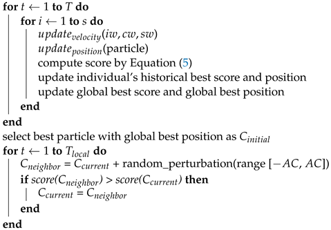
Electronics 13 04029 i001
C = C c u r r e n t
compute Y fusion by Equation (4)

3.2.2. GA-Based Control Gate Fusion

In this approach, the optimization process begins with initializing a population of candidate solutions, represented as individuals. Each individual, denoting a potential solution C, is characterized by a set of genes or parameters defining its properties. Over successive generations, the fitness function directs the evolution of the population via favoring and reproducing individuals with superior solutions. The optimization goal is to minimize accuracy loss in the pruned model, reflected in the fitness function defined in Equation (5).
During the iterative process, referred to as generations, individuals evolve through the application of genetic operators, including selection, crossover, and mutation. Selection plays a critical role, evaluating individuals based on their fitness, with those exhibiting higher fitness being more likely to be chosen for reproduction. Crossover, an intermediate step in GA, involves exchanging genetic information between parent chromosomes to generate offspring. In our approach, we select the two chromosomes with the highest fitness as parent individuals. We then randomly choose a crossover point along their binary strings and exchange the fragments after this point to create two offspring individuals. This operation combines advantageous genetic traits from different parents, potentially producing more promising solutions. Following crossover, genetic mutations are applied to the offspring chromosomes. Random bits within the binary strings are flipped, introducing diversity into the population and exploring new regions of the solution space. This mutation operation enhances the search process by introducing novel solutions and preventing premature convergence.
Through the iterative refinement of solution populations via selection, crossover, and mutation, the population gradually converges to solution C, closely mimicking the natural evolutionary process. Similarly, to prevent C from falling into a local optimum, a local search strategy is also introduced. The entire algorithmic process is summarized in Algorithm 2.
Algorithm 2: GA-Based Control Gate Fusion
Input: class-level control gate Y 1 , Y 2 , , Y V , populations, mutation rate m r , range of perturbation A C
Output:  Y fusion customized for targeted classes
generate_population (size = s)
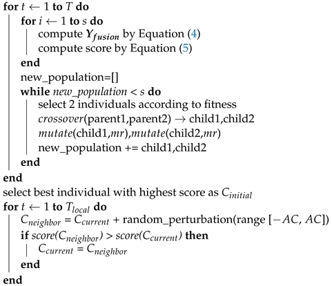
Electronics 13 04029 i002
C = C c u r r e n t
compute Y fusion by Equation (4)
    Using Y fusion , we selectively remove channels associated with low gate values, and thus, obtain a customized pruned model. As demonstrated in [45], a pruned model can achieve a comparable accuracy performance, regardless of whether it inherits weights from the original model. This implies that the core of channel pruning lies in identifying a well-performing pruning structure. As for its associated weights, we can perform fine-tuning before practical application on edge devices. This point is further confirmed by our simulation results. The procedure of TLCP is summarized in Algorithm 3.
Algorithm 3: Task-Level Customized Pruning
Input: Input image x of targeted classes, original model N
Output: Pruned model N p r u n e customized for targeted classes
Original prediction class i a r g m a x N ( x )
Electronics 13 04029 i003
Y v = i A i *
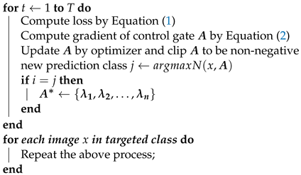
repeat for each class in targeted classes Y 1 , Y 2 , , Y V
Algorithm 1/Algorithm 2 c 1 , c 2 , , c V
Compute Y fusion by Equation (4)
Prune N N p r u n e

4. Results

In this section, we utilize the proposed method to customize VGG-16, ResNet-18, and ResNet-50. To evaluate the proposed method, we extensively perform experiments on three classification datasets: CIFAR-10, CIFAR-100, and ImageNet.

4.1. Performance Comparison

To verify the effectiveness of the proposed method, we compare the performance of TLCP with two baseline methods, i.e., (1) ResConv-Prune [46], which introduces a shortcut connection with a trainable information control parameter into a single convolutional layer, and (2) NNMP [17], which utilizes the training set to prune the model structure during training. This comparison focuses on the model pruning ratio on both the CIFAR-10 and CIFAR-100 datasets, as illustrated in Figure 6. The analysis provided in Figure 6a reveals the following insights. Firstly, our proposed method outperforms ResConv-Prune and NNMP by 29.0% and 10.1% on average, respectively, with improvements reaching up to 33.9% and 14.0% when the hyperparameter V is less than 6. This validates that TLCP effectively utilizes task information for model pruning, particularly when V is relatively small. However, as V becomes larger, the performance gains diminish. When V exceeds 6 and 8, TLCP is no longer superior to the baseline methods. This limitation is attributed to the linear fusion model adopted. As V increases, the control gates generated by simple linear fusion no longer accurately represent task information, necessitating a more sophisticated fusion model. Furthermore, the trend observed in the curve of TLCP indicates that as V increases, the pruning ratio decreases. This aligns with our intuition that more complex tasks necessitate more complex models. Similar results are observed on CIFAR-100, as illustrated by key data in Figure 6b. TLCP outperforms NNMP by 10.8% on average, with improvements of up to 20.4% when the V is less than 38. However, similar to results on CIFAR-10, the performance advantage of TLCP diminishes as V surpasses a specific threshold. This trend highlights a crucial limitation of the linear fusion model employed in TLCP. Specifically, as V increases beyond this threshold, the control gates generated by the simple linear fusion model struggle to accurately capture intricate task information. While TLCP is effective in leveraging task-level information for model pruning when V is relatively small, its performance diminishes as task complexity increases (i.e., with a larger number of targeted classes), necessitating a more sophisticated fusion model. This underscores a key observation: our proposed method excels in scenarios where V remains constrained. In these instances, TLCP effectively harnesses task-specific information, showcasing its effectiveness in optimizing model pruning. This highlights a nuanced strength of the proposed approach: it proves especially effective in situations where V leans towards the lower range of values, showcasing its optimal performance under such conditions. Under these conditions, the utilization of task-specific information is maximized, leading to enhanced model pruning outcomes.

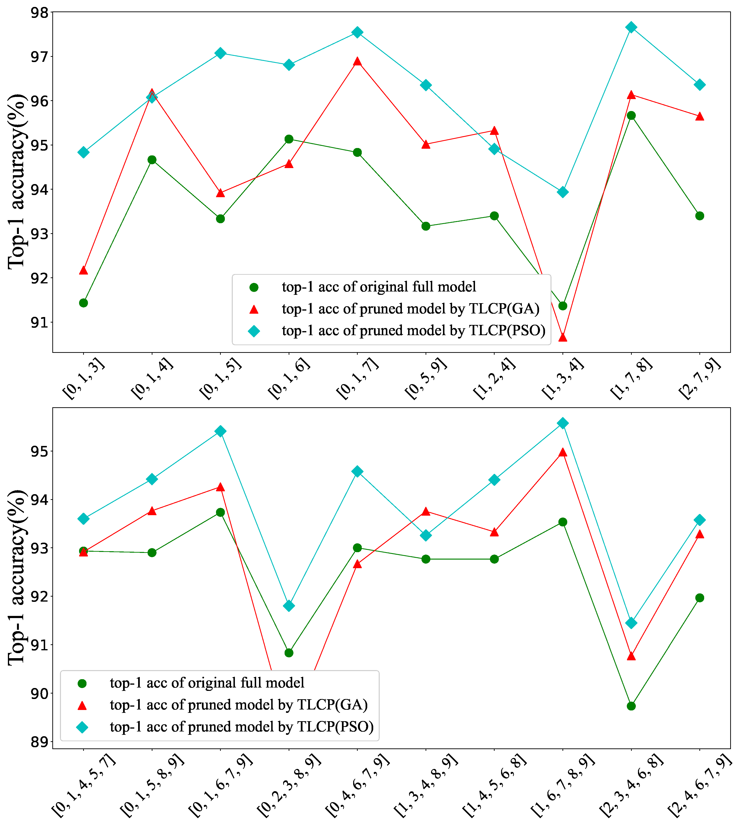
4.2. Choice of PSO or GA

In Section 3.2, we employ GA and PSO to fuse various class-level channel control gates. Figure 7 presents partial results of the performance of the pruned models generated by different methods for targeted class numbers 3 and 5. The experimental results indicate that for most class combinations, the pruned models obtained through PSO exhibit superior performance. This result can be attributed to PSO’s effectiveness in locating global optimal solutions, as particles rapidly converge near the optimal solution through information sharing. Furthermore, when dealing with a large number of targeted classes, high-precision solutions are needed to capture the details and characteristics of each gate. Given that GA requires more iterations and computational resources to find better solutions due to the larger solution space created by high-precision parameter representation, PSO outperforms GA in optimizing continuous parameters and can search the solution space with greater precision.
On the other hand, GA is comparatively more time-efficient during iterative exploration of the solution space. This effectiveness is also related to the selection of the chromosome occupancy. GA compromises on fusion granularity to achieve reduced fusion time, making it suitable for scenarios with stringent real-time requirements. Given the experimental results demonstrating PSO’s superiority in enhancing the performance of pruned models, our subsequent experiments are based on PSO.

4.3. Effect of Fine-Tuning

Figure 8 illustrates the impact of fine-tuning on the top-1 accuracy of the pruned model across different class combinations. Notably, our method shows a modest improvement in top-1 accuracy compared to the original full model. However, it is crucial to highlight that without the fine-tuning step, TLCP experiences a significant decline in top-1 accuracy. This observed phenomenon can be attributed to the inherent goals of TLCP, i.e., identifying parameters and structures that contribute less to the model’s performance, allowing for their safe removal. If the pruned model inherits all parameters from the original model, it may converge towards a local optimum, potentially affecting performance. Rather than entirely rebuilding the model, TLCP fine-tunes and prunes based on the original architecture. Experimental evidence demonstrates that adjusting and refining parameters based on the pruning architecture significantly improves the accuracy performance of the pruned model. In practical terms, this emphasizes the critical role of fine-tuning in the model deployment pipeline. While TLCP establishes an efficient pruning structure, fine-tuning is an essential step before deploying the model in real-world applications. Therefore, it is necessary to apply a small amount of additional training data to further train the pruned model before practical application.

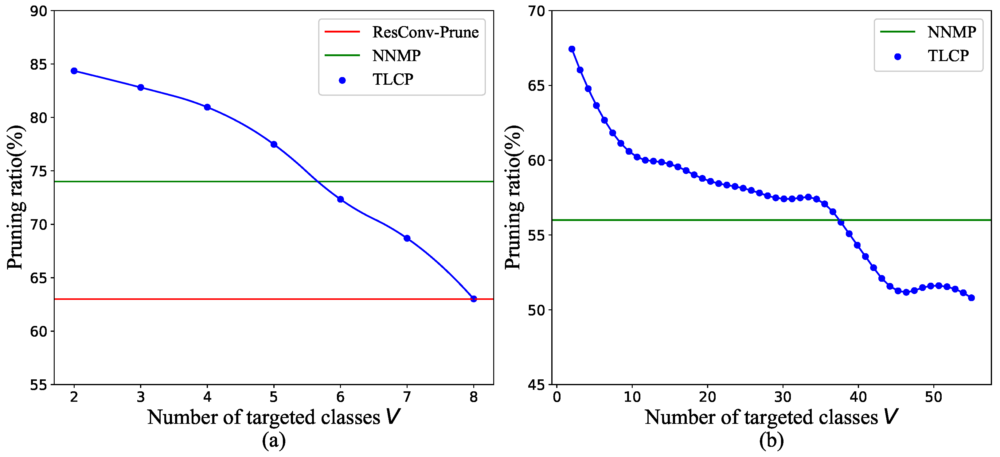
4.4. Relationship between Task and Model

Figure 9 presents the pruning ratio versus the number of targeted classes, under accuracy losses within 1% and 5% on CIFAR-10, CIFAR-100, and ImageNet. Here, accuracy loss refers to the difference in accuracy performance between the pruned model and original model. A consistent pattern observed across these datasets highlights a fundamental correlation: task complexity has a direct impact on the required number of model parameters. As task complexity increases, which means demanding a broader set of features and more nuanced information, the pruned model necessitates a higher number of parameters to effectively capture this diversity. Additionally, as the number of targeted classes (V) increases, the exclusivity or overlap between features becomes more pronounced. Certain features may be shared across multiple classes, while the importance of others may change in a nonlinear manner, complicating the fusion process. Linear fusion models, due to their intrinsic limitations, struggle to accurately capture these complex, nonlinear interactions, leading to a decline in both pruning effectiveness and overall model performance. For tasks with a larger V, we suggest exploring more advanced fusion models capable of capturing these complexities, thereby improving pruning efficacy. Nevertheless, designing such models poses significant challenges and represents a critical direction for future research.

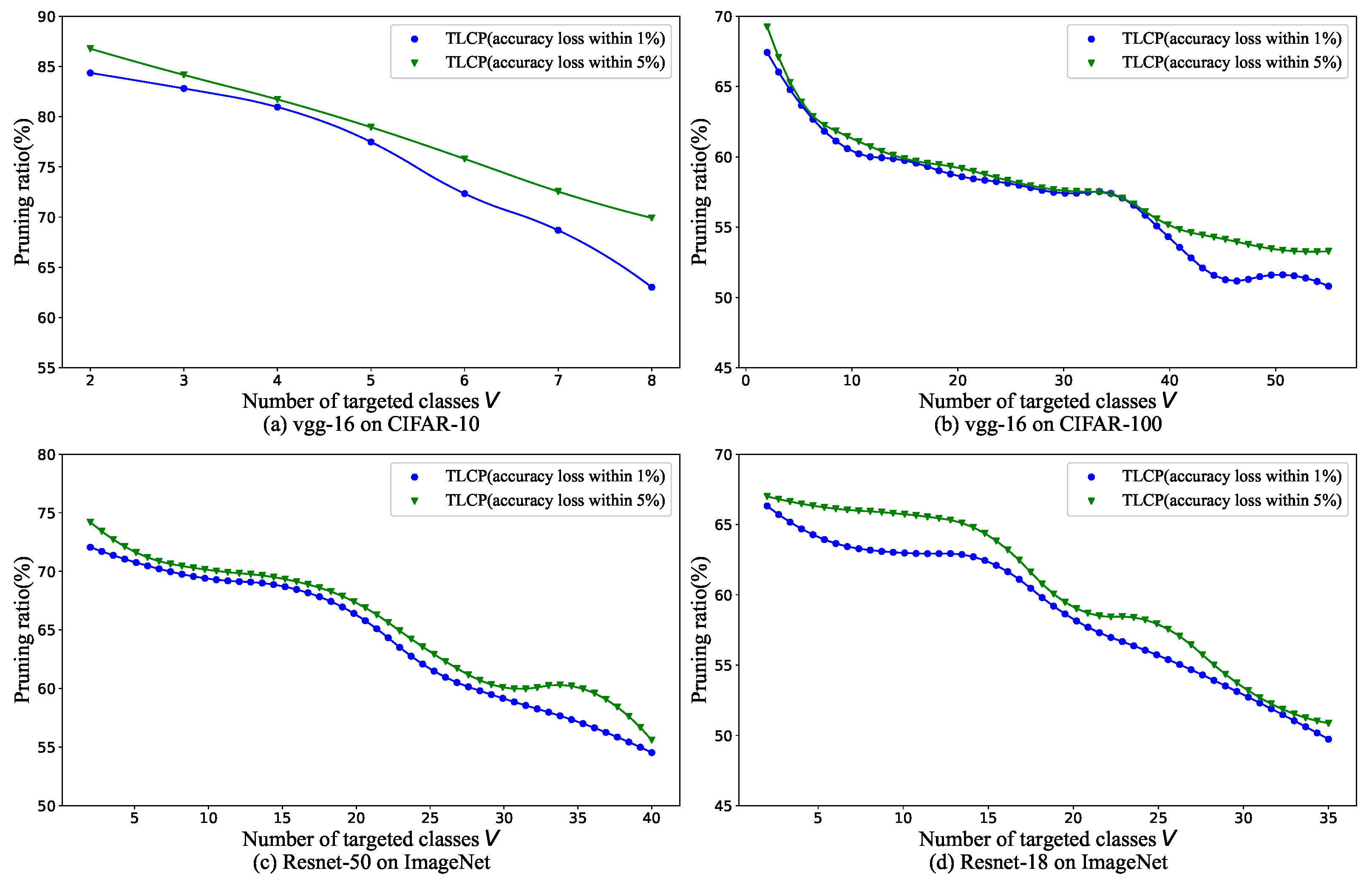
4.5. Trade-Off between Accuracy Loss and Pruning Ratio

Figure 10 shows the accuracy loss versus pruning ratio when the numbers of targeted classes are 3 (a), 5 (b), and 8 (c). When employing a lower pruning ratio, the accuracy of the pruned model may occasionally exceed that of the original full model. However, as the pruning ratio increases, a critical trade-off emerges, leading to a sharp increase in accuracy loss. This phenomenon can be attributed to the effectiveness of TLCP in removing redundant parameters, thereby enhancing accuracy performance under mild pruning scenarios. At lower pruning ratios, TLCP meticulously eliminates unnecessary channels, contributing to the superior accuracy of the pruned model compared to the original full model. As the pruning ratio escalates and more channels are pruned, a critical threshold is reached where the benefits of mild pruning are counteracted by the adverse effects of removing crucial channels from the original model. Consequently, accuracy loss becomes more pronounced, signifying the diminishing returns associated with aggressive pruning strategies. In practical terms, this emphasizes the intricate balance required in TLCP. While mild pruning can lead to a more efficient model with improved accuracy, aggressive pruning should be approached cautiously to prevent the inadvertent loss of critical information encoded in the model’s structure. These insights highlight the need for careful consideration of pruning strategies to achieve optimal trade-offs between model effectiveness and accuracy preservation in practical deployment scenarios.
It can be observed that across different scenarios with varying numbers of targeted classes, there exists a threshold for pruning. When the pruning ratio is below this threshold, the pruned model often achieves higher accuracy than the original full model. However, surpassing this threshold leads to a rapid increase in accuracy loss for the pruned model. The pruning threshold is different for different numbers of targeted classes, with scenarios featuring fewer targeted classes exhibiting a “later” appearance of the threshold. Tasks with a larger number of targeted classes tends to be more complex. Consequently, more complex tasks require lower pruning ratios to maintain accuracy. Under the same pruning ratio conditions, more complex tasks experience greater accuracy loss, aligning with our observations in Section 4.4.

4.6. Time and Memory

In this subsection, we assess the performance of the TLCP algorithm in terms of inference time and runtime memory usage across varying numbers of target task classes. Specifically, Table 1 presents a comparison of the inference time and memory utilization of the customized pruned model against the baseline VGG-16 model on the CIFAR-10 dataset, while Table 2 shows the results for ResNet-50 on ImageNet. Notably, the data in both tables indicate that TLCP-based pruned models achieve significant reductions in both memory usage and inference time. As the number of target task classes increases, the pruning ratio tends to decline. This trend arises because a higher number of classes introduces greater complexity in decision-making paths, necessitating the retention of more parameters to preserve inference accuracy, thus limiting the extent of pruning. Interestingly, the reduction in inference time does not exhibit a clear correlation with the number of target classes, remaining relatively stable across different class configurations. This stability is primarily attributed to the fact that inference time is not solely dependent on the pruning ratio, but also on hardware support for structured pruning and the architectural design of the model. Consequently, the optimization of inference time is more closely linked to hardware acceleration and model architecture rather than merely adjusting the pruning ratio. In summary, the performance of the TLCP algorithm in terms of inference time and runtime memory usage underscores its suitability for real-world edge deployments, effectively optimizing both metrics while preserving accuracy.

5. Discussion

Main contributions of TLCP: TLCP provides a valuable contribution to efficiently deploying CNNs in resource-limited environments, such as edge computing. It reduces computational and memory overhead while maintaining or improving inference performance, especially when only a small subset of image classes is needed. TLCP excels in cases where the number of targeted classes is low, making it well-suited for user-specific or application-specific tasks. Importantly, our method is not designed to compete with recent techniques like neural architecture search (NAS) and attention-based pruning, but to complement them by providing a novel perspective on reducing redundancy. While this work does not include direct integration with NAS [47] or attention mechanisms [48], we recognize that these approaches can be synergistically combined with our framework, which we view as a potential avenue for future exploration and process refinement.
Exploration of the fusion model: One key aspect of TLCP is the fusion of class-level control gates, which are combined to generate task-level control gates for effective pruning. We propose a linear fusion model, introducing a coefficient for each Y V to merge class-level control gates, simplifying training complexity and performing well with a small number of categories. Nevertheless, the exact mechanism of how class-level gates contribute to task-level gates remains unclear, requiring further investigation. Exploring nonlinear fusion models that take into account the varying contributions of different convolutional channels may enhance TLCP’s effectiveness in complex tasks. However, these advanced methods introduce additional computational overhead and training complexity, posing a trade-off that future research must address.
Adapting TLCP for unstructured data: challenges and potential. Although TLCP was initially designed for image data, its core mechanism of class-level control gates can theoretically be applied to unstructured data, such as point cloud data [49,50,51]. In TLCP, control gates can be optimized for multiple categories, with each category’s contribution being linearly combined to generate task-level control gates. However, unlike images, point cloud data often involve more complex geometric and spatial features shared across categories, necessitating the incorporation of nonlinear methods to better model their relationships. These nonlinear methods can significantly enhance the model’s expressive power but might also introduce additional computational overhead, which is crucial for real-time applications [52]. To sum up, the flexible gating mechanism of TLCP makes it a promising candidate for adaptation to unstructured data, provided that appropriate modifications are made to the model to address inherent differences in data structure. In particular, introducing nonlinear methods may be necessary to better capture relationships between categories.
In light of these considerations, future research could focus on developing task-level pruning frameworks specifically tailored for non-structured data. During the fusion process of class-level control gates, a finer-grained fusion approach can be employed in TLCP to capture nuanced interactions. The relationships between various class-level control gates remain unclear, representing an important area for future exploration. By leveraging inter-class relationships, we can develop a more interpretable approach for generating task-aware control gates, ultimately enhancing the effectiveness of pruning in non-structured data scenarios. Additionally, considering the evaluation of inference time and runtime memory usage of the pruned model in Section 4.6, we recognize the value of deploying TLCP on actual edge devices. This will be a priority in our future work to better assess its feasibility in real-world applications.

6. Conclusions

In this work, we introduce a novel task-level customized pruning method (TLCP), which leverages task-specific information to effectively reduce the complexity of CNNs. TLCP involves two key steps: firstly, generating class-level channel control gates to map class information onto control gates; secondly, utilizing PSO/GA to fuse class-level control gates, facilitating customized pruning. Simulation results demonstrate the efficacy of our approach in significantly reducing model size while maintaining competitive accuracy levels compared to baseline methods.

Author Contributions

Conceptualization: Y.W. and F.L.; supervision: Y.W. and H.Z.; methodology, collected the study data, formal analysis and writing—original draft: F.L. and B.S.; writing—review and editing: Y.W., F.L., H.Z. and B.S. All authors have read and agreed to the published version of the manuscript.

Funding

This work is supported in part by the National Key R&D Program of China (No. 2021YFB2900100), in part by the National Natural Science Foundation of China under Grant 62002293, in part by the China Postdoctoral Science Foundation under Grant BX20200280, in part by the Guangdong Basic and Applied Basic Research Foundation under Grant 2019A1515110406.

Data Availability Statement

Data are contained within the article.

Conflicts of Interest

The authors declare no conflicts of interest.

References

  1. Roy, S.K.; Deria, A.; Hong, D.; Rasti, B.; Plaza, A.; Chanussot, J. Multimodal Fusion Transformer for Remote Sensing Image Classification. IEEE Trans. Geosci. 2023, 61, 5515620. [Google Scholar] [CrossRef]
  2. Han, G.; Huang, S.; Ma, J.; He, Y.; Chang, S.F. Meta faster r-cnn: Towards accurate few-shot object detection with attentive feature alignment. In Proceedings of the AAAI Conference on Artificial Intelligence, Online, 22February–1 March 2022; Volume 36, pp. 780–789. [Google Scholar]
  3. Yuan, F.; Zhang, Z.; Fang, Z. An effective CNN and Transformer complementary network for medical image segmentation. Pattern Recognit. 2023, 136, 109228. [Google Scholar] [CrossRef]
  4. Krizhevsky, A.; Sutskever, I.; Hinton, G.E. Imagenet classification with deep convolutional neural networks. Commun. ACM 2017, 60, 84–90. [Google Scholar] [CrossRef]
  5. Simonyan, K.; Zisserman, A. Very deep convolutional networks for large-scale image recognition. arXiv 2014, arXiv:1409.1556. [Google Scholar]
  6. He, K.; Zhang, X.; Ren, S.; Sun, J. Deep residual learning for image recognition. In Proceedings of the IEEE Conference on Computer Vision and Pattern Recognition (CVPR), Las Vegas, NV, USA, 27–30 June 2016; pp. 770–778. [Google Scholar]
  7. Huang, G.; Liu, Z.; Van Der Maaten, L.; Weinberger, K.Q. Densely connected convolutional networks. In Proceedings of the IEEE Conference on Computer Vision and Pattern Recognition (CVPR), Honolulu, HI, USA, 21–26 July 2017; pp. 4700–4708. [Google Scholar]
  8. Peters, J.; Fournarakis, M.; Nagel, M.; Van Baalen, M.; Blankevoort, T. QBitOpt: Fast and Accurate Bitwidth Reallocation during Training. In Proceedings of the IEEE/CVF International Conference on Computer Vision, Paris, France, 2–6 October 2023; pp. 1282–1291. [Google Scholar]
  9. Chauhan, A.; Tiwari, U.; R, V.N. Post Training Mixed Precision Quantization of Neural Networks Using First-Order Information. In Proceedings of the IEEE/CVF International Conference on Computer Vision, Paris, France, 2–6 October 2023; pp. 1343–1352. [Google Scholar]
  10. Yang, G.; Yu, S.; Yang, H.; Nie, Z.; Wang, J. HMC: Hybrid model compression method based on layer sensitivity grouping. PLoS ONE 2023, 18, e0292517. [Google Scholar] [CrossRef]
  11. Savostianova, D.; Zangrando, E.; Ceruti, G.; Tudisco, F. Robust low-rank training via approximate orthonormal constraints. arXiv 2023, arXiv:2306.01485. [Google Scholar]
  12. Dai, W.; Fan, J.; Miao, Y.; Hwang, K. Deep Learning Model Compression With Rank Reduction in Tensor Decomposition. IEEE Trans. Neural Netw. Learn. Syst. 2023, 1–14. [Google Scholar] [CrossRef]
  13. Dai, C.; Liu, X.; Cheng, H.; Yang, L.T.; Deen, M.J. Compressing deep model with pruning and tucker decomposition for smart embedded systems. IEEE Internet Things J. 2021, 9, 14490–14500. [Google Scholar] [CrossRef]
  14. Gabor, M.; Zdunek, R. Compressing convolutional neural networks with hierarchical Tucker-2 decomposition. Appl. Soft Comput. 2023, 132, 109856. [Google Scholar] [CrossRef]
  15. Lv, X.; Zhang, P.; Li, S.; Gan, G.; Sun, Y. Lightformer: Light-weight transformer using svd-based weight transfer and parameter sharing. In Proceedings of the ACL, Toronto, ON, Canada, 9–14 July 2023; pp. 10323–10335. [Google Scholar]
  16. Liu, D.; Yang, L.T.; Wang, P.; Zhao, R.; Zhang, Q. TT-TSVD: A multi-modal tensor train decomposition with its application in convolutional neural networks for smart healthcare. ACM Trans. Multimed. Comput. Commun. Appl. 2022, 18, 1–17. [Google Scholar] [CrossRef]
  17. Xie, Y.; Luo, Y.; She, H.; Xiang, Z. Neural Network Model Pruning without Additional Computation and Structure Requirements. In Proceedings of the 2023 26th International Conference on Computer Supported Cooperative Work in Design (CSCWD), Rio de Janeiro, Brazil, 24–26 May 2023; pp. 1734–1740. [Google Scholar]
  18. Pietroń, M.; Żurek, D.; Śnieżyński, B. Speedup deep learning models on GPU by taking advantage of efficient unstructured pruning and bit-width reduction. J. Comput. 2023, 67, 101971. [Google Scholar] [CrossRef]
  19. Wang, C.; Zhang, G.; Grosse, R. Picking winning tickets before training by preserving gradient flow. arXiv 2020, arXiv:2002.07376. [Google Scholar]
  20. Zheng, Y.J.; Chen, S.B.; Ding, C.H.; Luo, B. Model compression based on differentiable network channel pruning. IEEE Trans. Neural Netw. Learn. Syst. 2022, 34, 10203–10212. [Google Scholar] [CrossRef] [PubMed]
  21. Zhang, Y.; Freris, N.M. Adaptive filter pruning via sensitivity feedback. IEEE Trans. Neural Netw. Learn. Syst. 2023, 35, 10996–11008. [Google Scholar] [CrossRef] [PubMed]
  22. Hanson, E.; Li, S.; Li, H.; Chen, Y. Cascading structured pruning: Enabling high data reuse for sparse dnn accelerators. In Proceedings of the 49th Annual International Symposium on Computer Architecture, New York, NY, USA, 18–22 June 2022; pp. 522–535. [Google Scholar]
  23. Ma, X.; Yuan, G.; Li, Z.; Gong, Y.; Zhang, T.; Niu, W.; Zhan, Z.; Zhao, P.; Liu, N.; Tang, J.; et al. Blcr: Towards real-time dnn execution with block-based reweighted pruning. In Proceedings of the 2022 23rd International Symposium on Quality Electronic Design (ISQED), Santa Clara, CA, USA, 6–7 April 2022; pp. 1–8. [Google Scholar]
  24. Guan, Y.; Liu, N.; Zhao, P.; Che, Z.; Bian, K.; Wang, Y.; Tang, J. Dais: Automatic channel pruning via differentiable annealing indicator search. IEEE Trans. Neural Netw. Learn. Syst. 2022, 34, 9847–9858. [Google Scholar] [CrossRef]
  25. Tian, G.; Chen, J.; Zeng, X.; Liu, Y. Pruning by training: A novel deep neural network compression framework for image processing. IEEE Signal Process. Lett. 2021, 28, 344–348. [Google Scholar] [CrossRef]
  26. Lei, Y.; Wang, D.; Yang, S.; Shi, J.; Tian, D.; Min, L. Network Collaborative Pruning Method for Hyperspectral Image Classification Based on Evolutionary Multi-Task Optimization. Remote Sens. 2023, 15, 3084. [Google Scholar] [CrossRef]
  27. Cong, S.; Zhou, Y. A review of convolutional neural network architectures and their optimizations. Artif. Intell. Rev. 2023, 56, 1905–1969. [Google Scholar] [CrossRef]
  28. He, Y.; Xiao, L. Structured Pruning for Deep Convolutional Neural Networks: A Survey. IEEE Trans. Pattern Anal. Mach. Intell. 2023, 46, 2900–2919. [Google Scholar] [CrossRef]
  29. Dong, Z.; Lin, B.; Xie, F. Optimizing Few-Shot Remote Sensing Scene Classification Based on an Improved Data Augmentation Approach. Remote Sens. 2024, 16, 525. [Google Scholar] [CrossRef]
  30. Liu, J.; Xiang, J.; Jin, Y.; Liu, R.; Yan, J.; Wang, L. Boost Precision Agriculture with Unmanned Aerial Vehicle Remote Sensing and Edge Intelligence: A Survey. Remote Sens. 2021, 13, 4387. [Google Scholar] [CrossRef]
  31. Wang, Y.; Li, F.; Zhang, H. TA2P: Task-Aware Adaptive Pruning Method for Image Classification on Edge Devices. In Proceedings of the ICASSP 2024–2024 IEEE International Conference on Acoustics, Speech and Signal Processing (ICASSP), Seoul, Republic of Korea, 14–19 April 2024; pp. 2580–2584. [Google Scholar]
  32. Yu, F.; Qin, Z.; Chen, X. Distilling critical paths in convolutional neural networks. arXiv 2018, arXiv:1811.02643. [Google Scholar]
  33. Wang, Y.; Su, H.; Zhang, B.; Hu, X. Interpret neural networks by identifying critical data routing paths. In Proceedings of the IEEE Conference on Computer Vision and Pattern Recognition, Salt Lake City, UT, USA, 18–23 June 2018; pp. 8906–8914. [Google Scholar]
  34. Li, Z.; Li, H.; Meng, L. Model Compression for Deep Neural Networks: A Survey. Computers 2023, 12, 60. [Google Scholar] [CrossRef]
  35. LeCun, Y.; Denker, J.; Solla, S. Optimal brain damage. Adv. Neural Inf. Process. Syst. 1989, 2, 598–605. [Google Scholar]
  36. Han, S.; Pool, J.; Tran, J.; Dally, W. Learning both weights and connections for efficient neural network. arXiv 2014, arXiv:1506.02626. [Google Scholar]
  37. Luo, J.H.; Wu, J.; Lin, W. Thinet: A filter level pruning method for deep neural network compression. In Proceedings of the IEEE International Conference on Computer Vision, Venice, Italy, 22–29 October 2017; pp. 5058–5066. [Google Scholar]
  38. Zhang, Y.; Wang, H.; Qin, C.; Fu, Y. Aligned structured sparsity learning for efficient image super-resolution. Adv. Neural Inf. Process. Syst. 2021, 34, 2695–2706. [Google Scholar]
  39. Fang, G.; Ma, X.; Song, M.; Mi, M.B.; Wang, X. Depgraph: Towards any structural pruning. In Proceedings of the IEEE/CVF Conference on Computer Vision and Pattern Recognition, Vancouver, BC, Canada, 17–24 June 2023; pp. 16091–16101. [Google Scholar]
  40. Beyer, L.; Zhai, X.; Royer, A.; Markeeva, L.; Anil, R.; Kolesnikov, A. Knowledge Distillation: A Good Teacher Is Patient and Consistent. In Proceedings of the IEEE/CVF Conference on Computer Vision and Pattern Recognition, New Orleans, LA, USA, 18–24 June 2022; pp. 10925–10934. [Google Scholar]
  41. Qiu, Y.; Leng, J.; Guo, C.; Chen, Q.; Li, C.; Guo, M.; Zhu, Y. Adversarial defense through network profiling based path extraction. In Proceedings of the IEEE/CVF Conference on Computer Vision and Pattern Recognition, Long Beach, CA, USA, 15–20 June 2019; pp. 4777–4786. [Google Scholar]
  42. Allen-Zhu, Z.; Li, Y.; Liang, Y. Learning and generalization in overparameterized neural networks, going beyond two layers. arXiv 2018, arXiv:1811.04918. [Google Scholar]
  43. Clerc, M.; Kennedy, J. The particle swarm-explosion, stability, and convergence in a multidimensional complex space. IEEE Trans. Evol. Comput. 2002, 6, 58–73. [Google Scholar] [CrossRef]
  44. Holland, J.H. Genetic algorithms. Sci. Am. 1992, 267, 66–73. [Google Scholar] [CrossRef]
  45. Liu, Z.; Sun, M.; Zhou, T.; Huang, G.; Darrell, T. Rethinking the value of network pruning. arXiv 2018, arXiv:1810.05270. [Google Scholar]
  46. Xu, P.; Cao, J.; Shang, F.; Sun, W.; Li, P. Layer pruning via fusible residual convolutional block for deep neural networks. arXiv 2020, arXiv:2011.14356. [Google Scholar]
  47. Lin, M.; Ji, R.; Zhang, Y.; Zhang, B.; Wu, Y.; Tian, Y. Channel pruning via automatic structure search. arXiv 2020, arXiv:2001.08565. [Google Scholar]
  48. Hossain, M.B.; Gong, N.; Shaban, M. A Novel Attention-Based Layer Pruning Approach for Low-Complexity Convolutional Neural Networks. Adv. Intell. Syst. 2024, 2400161. [Google Scholar] [CrossRef]
  49. Wang, C.; Ning, X.; Sun, L.; Zhang, L.; Li, W.; Bai, X. Learning discriminative features by covering local geometric space for point cloud analysis. IEEE Trans. Geosci. Remote Sens. 2022, 60, 5703215. [Google Scholar] [CrossRef]
  50. Zhang, H.; Ning, X.; Wang, C.; Ning, E.; Li, L. Deformation depth decoupling network for point cloud domain adaptation. Neural Netw. 2024, 180, 106626. [Google Scholar] [CrossRef]
  51. Fang, Z.; Li, X.; Li, X.; Buhmann, J.M.; Loy, C.C.; Liu, M. Explore in-context learning for 3d point cloud understanding. arXiv 2023, arXiv:2306.08659. [Google Scholar]
  52. Cui, Y.; Chen, R.; Chu, W.; Chen, L.; Tian, D.; Li, Y.; Cao, D. Deep learning for image and point cloud fusion in autonomous driving: A review. IEEE Trans. Intell. Transp. Syst. 2021, 23, 722–739. [Google Scholar] [CrossRef]
Figure 1. An example of the importance of neurons for different classes.
Electronics 13 04029 g001
Figure 2. The framework contains two phases, i.e., mapping of image information to channel control gates (phase one) and class-level control gate fusions (phase two). For each input image, TLCP introduces a control gate associated with each layer’s output channel to quantify contributions of different channels. The mapping process from image information to control gate is completed in phase one. In phase two, we combine control gates corresponding to the targeted classes using a linear fusion model. For task-aware customized control gates, we perform pruning based on the gate value.
Electronics 13 04029 g002
Figure 3. Control gates are multiplied by the layer’s output, a smaller gate value means the associated channel contributes less to the final model prediction; removing such channels has little effect on the model’s inference performance.
Electronics 13 04029 g003
Figure 4. Comparison of control gate values across all convolutional filters in the 3rd (a) and 7th (b) convolutional layers of VGG-16 on CIFAR-10 for all-class input. Comparison of control gate values across all convolutional filters in the 3rd (c) and 7th (d) convolutional layers of VGG-16 on CIFAR-10 for class 3 input. Bright and dark colors indicate high and low gate values, respectively.
Electronics 13 04029 g004
Figure 5. An example of three-class fusion. Given three targeted classes, we introduce a coefficient c i for each Y v and adopt a linear fusion model to merge different class-level control gates.
Electronics 13 04029 g005
Figure 6. Pruning ratio comparison under different numbers of targeted classes on (a) CIFAR-10 and (b) CIFAR-100.
Electronics 13 04029 g006
Figure 7. Comparison of TLCP based on PSO (Algorithm 1) and GA (Algorithm 2) under different class combinations.
Electronics 13 04029 g007
Figure 8. Effect of fine-tuning under different class combinations when pruning ratio is 0.82.
Electronics 13 04029 g008
Figure 9. Pruning ratios versus the number of targeted classes under accuracy drop within 1% (blue) and 5% (green) for (a) VGG-16 on CIFAR-10, (b) VGG-16 on CIFAR-100, (c) ResNet-50 on ImageNet, and (d) ResNet-18 on ImageNet.
Electronics 13 04029 g009
Figure 10. Accuracy loss versus pruning ratio when the numbers of targeted classes are 3 (a), 5 (b), and 8 (c).
Electronics 13 04029 g010
Table 1. Inference time and memory usage comparison: Customized pruned model vs. baseline VGG-16 model on CIFAR-10 1.
ModelNumber of Targeted ClassesPruning Ratio (%)ParametersTime Reduction (%)
Baseline Model--17.53 M-
Pruned Model284.364.04 M27.41
Pruned Model382.814.38 M26.10
Pruned Model480.964.58 M26.87
Pruned Model577.485.08 M25.37
Pruned Model672.346.13 M26.09
Pruned Model768.696.83 M25.72
1 The results are the average of 50 experiments, and the batch size used is 128.
Table 2. Inference time and memory usage comparison: Customized pruned model vs. baseline ResNet-50 model on ImageNet 1.
ModelNumber of Targeted ClassesPruning Ratio (%)ParametersTime Reduction (%)
Baseline Model--23.71 M-
Pruned Model570.798.24 M21.93
Pruned Model1069.378.58 M19.41
Pruned Model1568.748.73 M21.92
Pruned Model2066.298.97 M18.76
Pruned Model2561.6810.02 M20.02
Pruned Model3059.1310.91 M19.06
Pruned Model3557.1611.15 M18.02
1 The results are the average of 50 experiments, and the batch size used is 64.
Disclaimer/Publisher’s Note: The statements, opinions and data contained in all publications are solely those of the individual author(s) and contributor(s) and not of MDPI and/or the editor(s). MDPI and/or the editor(s) disclaim responsibility for any injury to people or property resulting from any ideas, methods, instructions or products referred to in the content.

