Abstract
Labeling-Based Recipient Identification (LABRID) brings the possibility of representing the destination station address in a Bit-Interleaved Coded Modulation with Iterative Decoding (BICM-ID) system by a signal labeling rule. Low-order modulations, such as BPSK or QPSK, pose a general problem for BICM-ID due to a limited convergence of iterative decoding. In the context of LABRID, they have one more drawback—a small number of different labeling rules in general; the number of the optimal ones, which exhibit the maximal asymptotic coding gain, is reduced even further. Meanwhile, LABRID needs a sizable collection of different optimal labeling rules to serve many users in large wireless networks. In this paper, the author suggests the use of hypercube BPSK or QPSK labeling to overcome all these challenges. By means of the Reactive Tabu Search (RTS) algorithm, more than 1500 equivalent optimal hypercube labeling rules are found. Analytical error bounds of the system are developed and supported by simulation experiments. Then, the focus is moved to the criterion to determine the frame destination at the LABRID receiver; a simple threshold-based method is proposed to keep the incorrect decision probability below . Finally, it is shown that LABRID outperforms a reference BICM-ID system in terms of computational complexity.
1. Introduction
1.1. LABRID at a Glance
BICM-ID [1] is a variation of BICM [2,3], in which the receivers, similar to turbo decoders, can gradually improve the reliability of data estimates thanks to the iterative decoding procedure. In greater detail, the demapper and channel decoder exchange their bitwise log-likelihood beliefs on codeword bits with each other. For the process to be successful, a specific signal labeling map (or labeling, for brevity) must be used for mapping the interleaved codeword bits onto constellation points at the transmitter—it should exhibit a high asymptotic coding gain.
LABRID has been invented as a method for physical-layer addressing in wireless communications without the explicit sending of any address. Instead, the recipient ID is reflected by a unique signal labeling map. LABRID draws its strength from the observation that the iterative process at the BICM-ID receiver does not converge unless the labeling map used at the transmitter side suits the one assigned to the considered demapper. Any foreign frame (i.e., a frame destined for another recipient), can therefore be easily discriminated against due to its lack of convergence decoding, which can be detected using simple threshold-based methods—in [4] it was proposed to measure the absolute extrinsic log-likelihood ratio (LLR) mean at the demapper output, related to the codeword bits, in the last executed decoding iteration (however, one can take into consideration different measures available at the receiver, like the mutual information estimates). Hence, the decision to reject foreign frames is made in the physical layer with only marginal computational cost of obtaining a mean. For the frames identified as foreign, there is no need to run a decoding pass in the last iteration. In contrast, for conservative Medium Access Control (MAC) addressing, the likelihoods of data bits are indispensable for both desired and foreign frames, and every decoded data frame is transferred to the MAC layer, where it undergoes integrity checking, after which the destination address might finally be read.
Along with reasonable computational payload reduction, LABRID offers a small improvement in the data rate, as there is no need to spend any bit to carry the recipient address. However, to be fair, this might be relevant only for very short data frames, which, in turn, are not preferred for BICM-ID systems due to the deficit of decoding convergence. This deficit is caused by the fact that the a priori LLRs on subsequent codeword bits are not sufficiently independent from the extrinsic decisions made about them in the previous iteration.
In Ref. [5], it has been shown that the LABRID receiver can effectively work in a “heterogeneous” environment, in which the signals of different modulation order are transmitted. In addition, the LABRID receiver demonstrated its capability of rejecting legacy BICM frames, in which the typical Gray labeling was used.
1.2. LABRID in Comparison with Other Techniques
LABRID has emerged from BICM(-ID), like many other novel transmission concepts. Therefore, for the reader’s better orientation, let us consider LABRID against the background of a few competing techniques.
There are some BICM-ID enhancements, like signal-space diversity (SSD) [1] or Constellation Shaping (CS) [6,7], which aim to increase the asymptotic coding gain over that of the original BICM-ID or move the position of the turbo cliff. Actually, LABRID does not assume either signal component interleaving (as for SSD) or re-designing the signal constellation (as in the case of CS). Instead, the regular 16-QAM constellation of equiprobable points, and the error probability measures are the same as for the original BICM-ID.
LABRID can be wrongly seen as a flavor of the popular Index Modulation (IM) [8,9], where the so-called Virtual Bits determine the resources selected to transmit subsequent portions of data. The resources considered to be used with IM are, e.g., RF chains, signaling intervals, OFDM subcarriers, or even I-Q signal components. The recipient address, represented by a labeling map according to the LABRID concept, seems to be similar to Virtual Bits, which are not explicitly transmitted according to IM techniques. But note the significant difference: LABRID does not determine any selection of available resources according to the given recipient ID—all resources are still in use. What actually undergoes any manipulation in the case of LABRID is the way of bit mapping onto constellation points, with no impact on the system diversity order.
The result of LABRID use seems to be comparable to the application of scramble coding, known, e.g., from 3G telecommunication systems. In fact, the bit stream scrambled with one scrambling code is weakly correlated with that using another scrambling code. However, LABRID has nothing in common with spectrum spreading—it does not have an impact on the shape of the signal spectrum.
1.3. Research Problem Formulation
LABRID requires a sizable number of different labelings to serve a reasonable number of users. In addition, it is not enough to take into account any set of labeling maps for a given modulation order. Not only should the good labelings yield a high asymptotic coding gain over the (noniterative) Gray-labeled BICM, but also they must be not similar to each other (e.g., exchanging two constellation points’ labels with each other cannot be considered a significant difference). Therefore, the author in [4] focused on a set of 768 -compliant 16-QAM labelings, all of which exhibit identical high-rank asymptotic coding gain. The results presented in [4] are entirely satisfactory: none of the users are discriminated against in terms of the iterative decoding results, and the receivers can correctly assess the destination of every single frame, judging by the observed convergence of the iterative process. In addition to 16-QAM, LABRID has also been studied along with 64-QAM BICM-ID with a similar, positive result [10].
For any BICM-ID system, a factor that affects the effectiveness of iterative decoding is the average distance between constellation points that differ in exactly one bit position [11]. According to widespread Gray labeling, the Hamming distance between the labels associated with neighboring constellation points is 1, which is the poorest case from the BICM-ID point of view. In general, the number of possible labelings (i.e., the ways in which binary labels can be assigned to the constellation points) is the factorial of modulation order. For better clarification: the number of candidate labelings that promise good iterative decoding performance is even smaller. Note that for low-order modulation the limit is very strict; there are only two different labelings for BPSK and for QPSK. For BPSK, bit 0 can be assigned to the constellation point and bit 1 to or vice versa. None of such two labelings can achieve any benefit from iterative decoding, as both are of the Gray type. In the case of QPSK, any labeling can be of either Gray or natural type. The Gray labelings, just like for higher-order modulations, are not worth being considered as candidate BICM-ID labelings. The natural labelings exhibit only a little gain over Gray when applied in a BICM-ID system [12]. In this light, it seems as if BICM-ID was useless in the case of low-order modulations.
Another problem appears if one aims to incorporate LABRID into QPSK BICM-ID; there are only 12 equivalent natural labelings (recall the two groups of QPSK labelings, mentioned above)—not enough for any practical use of LABRID. For BPSK the situation is even worse, as there are only two different labelings at all, none accurate for iterative decoding purposes. The question then arises whether LABRID can be used together with modulations having modulation order below 16.
The solution to the problem of poor BICM-ID performance in the case of low-order modulations was developed a couple of years ago; the so-called hypercube (or multidimensional) labeling. It consists in mapping binary tuples onto a series of symbols of the given modulation, thereby increasing channel diversity. It does not affect the data rate. In particular, for the BPSK hypercube labeling, there is still one bipolar symbol to be transmitted within one modulation period, but the values of subsequent symbols no longer depend solely on individual codeword bits. In [12], the authors developed the optimal QPSK 4-cube labeling, i.e., an assignment of 4-bit labels to pairs of QPSK symbols, whose elements are to be transmitted within two subsequent modulation periods (note that the real and imaginary components of a QPSK symbol constitute separate hypercube dimensions). Then, in [13] they considered the optimal 4-cube and 6-cube labeling for BICM-ID over different channels. In parallel, in [14] a larger variety of hypercubes consisting of QPSK or BPSK symbols was considered for transmission over the AWGN channel. In the current paper it is shown that hypercube labeling brings the possibility to merge the novel LABRID concept with low-order modulations. Indeed, thanks to the use of a general-purpose optimization algorithm, the author found more than 1500 equally good hypercube labelings of QPSK and BPSK symbols—so needed to enable physical layer recipient addressing. The other outcomes of the research are as follows: derivation of the analytical error bound of the considered system, and a proposal of a simple threshold-based criterion for assessing frame destination.
1.4. Paper Structure
The organization of this paper is as follows. Section 2 introduces the system model and describes frame filtering—the method for distinguishing foreign and desired frames. Section 3 covers the theoretical aspects of LABRID BICM-ID error bounds, specifies the requirements that should be met by the optimal hypercube labelings, and delivers exemplary outcomes of the optimization algorithm used to find them. In Section 4, the results of an overall LABRID system simulation experiment are presented and verified by means of the EXIT chart [15,16] and compared with analytical bounds. The efficiency of frame filtering is studied, and the computational cost is delivered therein. Finally, Section 5 concludes the work.
1.5. Notations
Scalars are denoted by italic letters, whereas vectors and matrices are denoted by bold-face letters (bold-face italic in the case of real or complex data type). and represent the -dimensional space of real, and complex numbers, respectively. means the -dimensional Boolean space. stands for the real part. and mean complex conjugate and the vector/matrix transpose, respectively. represents an identity matrix, while is the imaginary unit. denotes the statistical expectation. The expression ∼ means that the given random variable is distributed normally with mean, 0, and variance, .
2. LABRID for BICM-ID with Multidimensional Labeling
2.1. System Model
The considered LABRID BICM-ID system model is shown in Figure 1.
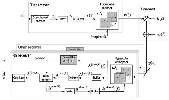
Figure 1.
Model of BICM-ID system employing LABRID and multidimensional labeling.
Data frame of length , denoted by , is encoded by a convolutional encoder employing the short code, which is a common choice for BICM-ID. The resultant codeword is passed through a pseudo-random bitwise interleaver of depth equal to the codeword size. The interleaved codeword is then buffered and cut into binary blocks of length where is the time offset of a given block. Each block is mapped onto a 4-cube vertex according to a labeling map
Depending on the modulation type, the elements of belong to either BPSK signal set: or QPSK signal set: .
Conforming to LABRID principles, the hypercube labeling map, , is recipient-specific. While running in the real system, the recipient ID, , is dropped down from the MAC layer to the physical layer. Vertices are transmitted through the uncorrelated Rayleigh fading channel, so that the received vector
Due to the assumption of coherent detection, the elements of are modeled as real i.i.d. Rayleigh RVs, all having zero mean and unitary variance; the elements of represent the samples of additive white Gaussian noise with zero mean and variance of in either real or imaginary dimension (the complex channel model is valid for either QPSK and BPSK transmitted symbols). Note that the signal reaches many receivers simultaneously; only one of them is the desired frame recipient. With no generality loss, we can assume identical channel realization for each receiver, as the role of a given station might change from one event of frame transmission to another.
At the considered th receiver, using labeling map , the hypercube demapper computes the extrinsic LLRs (i.e., log-likelihood ratios) individually per codeword bit of block as
where is a hypothetically considered binary block of length , having on bit ,
is a vertex assigned to according to the labeling . is the norm in induced by the inner product
so that . The a priori demapper information, is gleaned from the Soft-Input Soft-Output (SISO) decoder [17].
The individual extrinsic demapper LLRs are merged into vectors
related to respective binary blocks , and then into vector
including the extrinsic demapper LLRs for all bits of the codeword. Then the elements of are deinterleaved to constitute , i.e., the input information of the SISO decoder. Taking into account the code rate of , there are LLRs related to the codeword bits per each th trellis section: , which constitute a vector such that
With no generality loss, let us assume that the decoder operates according to the max* principle. It can represent the accurate optimal log-MAP routine, simplified approach with the use of look-up tables as corrections, or the basic max-log-MAP, deriving its simplicity from the Jacobi logarithm approximation [18].
The decoding process in each iteration consists of four phases [17]:
2.1.1. Calculation of Edge Transition Cost
The transition cost is obtained for each edge in every th trellis segment as
where are the subsequent codeword bits assigned to the trellis edge .
2.1.2. Calculation of State Metrics in the Forward Trellis Pass
The forward metric of state in the trellis segment is calculated recursively as
where and are the origin and destination state of edge , respectively. To break the recursion loop, it is assumed that the encoder starts the encoding process in the all-zero state.
2.1.3. Calculation of State Metrics in the Backward Trellis Pass
Similarly to (10), one can obtain the metric of state in the th trellis segment as
Since the encoder appends a respective number of tail bits to the data frame, the backward trellis pass starts at the all-zero state.
2.1.4. Generation of LLRs
For all but the last decoding iteration, the decoder generates the extrinsic codeword-related LLRs as
They are the elements of vector such that
Passed through the interleaver, becomes a priori demapper information,
in the next iteration.
In the last decoding iteration, the decoder delivers the extrinsic LLRs associated with the data bits (one bit per one trellis segment):
where is the data bit assigned to the trellis edge . Subsequent LLRs from (15) constitute vector
which is, finally, passed through a quantizer to obtain an estimated data frame,
Note that in the LABRID receiver, the last-iteration decoder pass is not run for any foreign frame, which significantly reduces the computational payload.
2.2. Frame Filtering
LABRID receivers are equipped with a frame filter, necessary to reject the frames which are not actually destined for them. The frame filter makes use of the author’s observation that the iterative decoding process in any BICM-ID receiver can converge only if both conditions are met:
- is high enough,
- the demapper labeling map is identical to the map used at the transmitter [4].
Convergence means that the mutual information between the codeword and the extrinsic demapper or decoder LLRs increases within subsequent decoding iterations; the LLRs become more and more reliable from one iteration to another. Fortunately, there is no need to compute mutual information explicitly, as the reliability of any LLR strictly corresponds to its magnitude [19]. Consequently, the LABRID receiver computes the absolute extrinsic demapper LLR mean per frame, denoted by , hereinafter, and compares it against a threshold value , empirically specified. The main reason for choosing the values of the extrinsic demapper LLRs as the frame filtering criterion instead of the extrinsic decoder LLRs is that it might save the time necessary for decoder’s operation in the last iteration when the frame is classified as foreign. Obviously, there is a nonzero probability that a frame that is actually destined for the considered receiver (called a desired frame, hereinafter) is wrongly classified as a foreign frame (i.e., directed to the other receiver). Such an error event will be termed misdetection. Another kind of error (called false alarm) appears if the receiver makes the decision to acquire a foreign frame.
With the aim of formalizing the probability of both types of errors, mentioned above, let be the pdf of the value of at the considered , given the labeling map used on the transmitter side. The misdetection event at the th receiver appears if the labeling used on the transmitter side is identical to labeling used by the considered receiver and falls below the threshold at the same time. Thus, the respective probability of misdetection error (or Misdetection Rate, MR) at the th receiver reads
By averaging over all possible labeling maps, one obtains
which seems to be a more valuable measure of frame filtering efficacy. However, all the optimal labelings—by definition—exhibit exactly the same features, so the MR calculated for any receiver gives the value of the general MR. In other words, the conditional pdfs are identical for all equivalent labelings. Consequently, to calculate MR, one can assume any optimal labeling per frame, necessarily the same at both sides of the system, which is represented by condition in the final MR definition:
By analogy to MR, let us define False Alarm Rate (FAR) as
where the condition is that the receiver labeling is different from that used on the transmitter side, though both are equivalent optimal labelings.
The definitions of MR and FAR will be used in the experimental part (Section 4.4) to determine the optimal threshold values per the assumed values of .
3. Optimal Hypercube Labeling Set
3.1. Error-Free Feedback BER Bound
BICM-ID achieves the Error-Free Feedback (EF) state having performed a sufficient number of iterations, unless is too low for the iterative process to converge. Consider the binary blocks and , which are identical except for bit . The results of and mapping into the -cube are the and vertices, respectively. The elements of and are regular constellation points of BPSK (in such a case, ) or QPSK (), which means that a binary vector of length can be mapped onto a sequence of 4 BPSK signals or 2 QPSK signals. Note the same hypercube size (or number of dimensions) in both cases. Let be the actually transmitted symbol. For the EF case in BICM-ID, the demapper’s decision on the th bit of block mapped onto is incorrect if the distance of the received vertex from is longer than that from competing vertex (all other competing vertices can be expurgated, since all remaining bits of are assumed to be ideally estimated [1]). Accordingly, let us consider the metric difference between and when is received, given the current channel state and noise vector . Unlike for the regular BICM-ID system from [1], the metric difference reflects hypercube labeling (for brevity, let be replaced by when considering a given pair):
Repeated use of the following features of the inner product:
and
gives
Since
and
it can be observed that
where
Note that (25) is valid only in the case of coherent detection, which allows for the assumption that .
Given , metric difference is a linear combination of two i.i.d. RVs: and—as such—is the Gaussian RV, too. From it can immediately be inferred that the mean of is
Accordingly, the variance of yields
where
Since the real and imaginary noise components are mutually independent,
In this position, to obtain and it is enough to take into account that by definition Knowing that , one obtains , and then
For the future use let us specify the bilateral Laplace transform of the pdf of the metric difference from (20):
For the given , since , all terms are i.i.d. Gaussian RVs, so
Since for any Gaussian RV , it is also valid for every :
Taking into account that the individual elements of are i.i.d. RVs,
In (37), one can recognize the moment generating function (MGF) of a normalized Rayleigh-distributed RV , which yields
The convergence criterion of MGF is . Accordingly, by assigning
one finally arrives at
The obtained Laplace transform (40) has purely real poles, i.e., there is an
pair for each , and it can converge in the region where
Note that the restriction of to that interval is a real, positive and convex function with the minimum at for any pair.
Now, let us study the overall system performance. Consider subsequent bits of the codeword: , each equally likely to be 0 or 1 (). After interleaving, they are mapped onto random positions of the labels of randomly selected vertices constituting a sequence . That is, bit is mapped onto position of the label of vertex and so on. Then, let be a sequence of vertices , whose labels are identical to those of except for the positions , respectively. For the given codeword, the error event of Hamming distance occurs when the cumulative metric difference
Having said this, recall the EF BER bound for a BICM-ID system employing a rate- convolutional code [1,2]:
where is the total input weight of the error events at Hamming distance , is the free distance of the code, and is the set of all hypercubes. The pairwise error probability (PEP)
A general formula for , derived in [20], is
where
is the bilateral Laplace transform of the cumulative metric difference and belongs to the intersection of the regions of convergence of all terms with the real positive line. The last transformation in (44) is valid as all terms are mutually independent RVs. Consequently,
where (a) is valid because all and RVs are mutually independent, and (b) is obtained because of the identical (uniform) probability distribution of all ’s and the same for all ’s. Computing the integral from (45) seems to be a challenging task; the author of the paper applies a method based on numerical integration, detailed in (Section 13.3.2 in [21]).
The developed tight EF bounds will be used in the further part of the paper to verify the accuracy of simulation experiments.
3.2. Properties of Optimal Hypercube Labeling
The tight EF bounds are quite impractical when comparing different labeling maps in terms of their impact on PEP. Therefore, let us resort to the loose Chernoff PEP bound (Sections 12.1.1, 13.3 and 13.5 in [21]):
Now, it is easy to determine the impact of the constellation type and labeling on the system performance by introducing a distance parameter
It is clear that is proportional to , so the optimal hypercube labeling map for the given hypercube is
In [12], the authors considered the optimal labeling map for the case of an -cube consisting of QPSK signals. However, their approach was more general, as they focused on hypercube dimensions rather than component signals. In particular, the 4-cube is made up of four orthogonal coordinates, which may represent either four subsequent BPSK symbols or two pairs of real and imaginary QPSK symbol components. Consequently, let us represent the vertices by a series of coordinates: by , and by . The individual elements of and will be referred to using index .
The distance parameter (47), expressed explicitly with the coordinates, takes a different form for the two hypercube variants, i.e.,
and
for BSPK and QPSK, respectively.
Let us consider the distances between vertices and , whose labels ( and ) differ at position . Having hypercube dimensions, the same or opposite coordinates for and can be assigned in any dimension, as
Consequently, the distance between and can be either 0 or .
Let us define a set containing all one-dimensional distances for a given pair
and respective Euclidean distance
As one is interested in maximizing the actual distance parameter related to labeling (47), they should maximize for all vertices and all , regardless of the hypercube variant considered. It would be achieved if the vertices and differed from each other in all dimensions, for every , so that and . But here the constraints caused by the hypercube properties must be taken into account [13]. That is, for a given , the desired content of can appear only for one value of . To better explain it, without loss of generality, let be assigned to a binary block = . It is obvious that there is only one competing vertex, i.e., , with the highest distance from . It can be labeled, e.g., by , so let us call it . Now let us consider the remaining second furthest vertices that can be assigned to the other binary blocks at Hamming distance 1 to (, , ). There are four equally good candidates: the vertices differing in three out of four coordinates from , namely . Each of them yields and . To conclude this part, let us formulate Corollary 1.
Corollary 1.
For the best 4-cube labeling in the BICM-ID system, a distance spectrum
contains the entries for every vertex
The corollary reflects the limits caused by the construction of the 4-cube. Any labeling that conforms to these limits will be considered the ideal labeling. However, in advance, it is not guaranteed that one exists. Note that Corollary 1 is valid for both BPSK and QPSK constellations used to create the 4-cube. In (53), there is only one entry bigger than the rest—in the case of the QPSK constellation it might be a real or imaginary component of either the first () or the second symbol of the vertex. The final assignment has no impact on the content of .
Now, let us recall (50)—the distance parameter for QPSK—in the context of the considered example. For the most distant competing vertex, both component QPSK signals differ from their counterparts in both real and imaginary coordinates. Meanwhile, for the remaining three competing vertices (with the second furthest distance), one of the coordinates (real or imaginary, of either the first or second component QPSK signal) is the same as for . In the case of the ideal labeling (constrained only by the properties of the hypercube), the same pattern appears for every vertex . Consequently, the limit for any QPSK hypercube labeling is constituted by
where the distance of 8 represents the case where both QPSK coordinates of are different from their counterparts , and 4 appears for the cases where only one coordinate (real or imaginary) is different. The last transition results from the assumption that the optimal distance pattern features in every , so the expectation over disappears. For , one can assume which yields a simpler loose bound:
In the case of a hypercube based on BPSK symbols, the individual hypercube coordinates are de facto single BPSK symbols, transmitted during separate modulation intervals. Consequently,
Again, for
If one assumes reasonably small and when comparing the approximate minimal values of and , they obtain
The ratio becomes smaller and smaller with decreasing . This is a clue that the considered system exhibits better asymptotic performance when employing BPSK hypercube labeling; the cost is a halved data rate.
3.3. Search for the Optimal Hypercube Labeling
In [13], an algorithm was developed to obtain the best labeling for a hypercube of any dimension . For the case of , it complies with the ideal labeling conditions, specified by Corollary 1. However, for LABRID applications, one needs hundreds of such optimal labelings. One way to generate such a labeling set is to start with the optimal labeling from [13] and consider some assignment manipulations. Another solution is to start from scratch and utilize adequate optimization algorithms, such as the Binary Search Algorithm [22], or Reactive Tabu Search (RTS) [23], commonly used to solve combinatorial problems, such as label assignment in BICM-ID. In a general case, the advantage of the second approach is that it is not constrained by the outcomes of the previous contributions and allows the exploration of new areas of the search space. However, in the considered case, no optimal labeling can break the rules specified for the ideal labeling in Corollary 1, so the optimal solution can be easily identified.
Having taken into account the above remarks, the author decided to run the RTS algorithm, which has been successfully used in the past to find equivalent optimal labelings for 16-QAM [4] and 64-QAM [10]. The optimization goal is to minimize the distance parameter (47), which represents the impact of labeling on system performance, and acts as the cost function for the optimization algorithm. It is instantiated for QPSK and BPSK hypercubes in (50) and (49), respectively. When searching for the optimal labeling map at , a reasonably small (i.e., 0.1) is assumed in the cost function. Every labeling visited by the RTS algorithm is checked for compliance with Corollary 1. If the labeling passes the check and has not been found before, it is archived, and the algorithm starts another optimization round from the initial random labeling assignment. After an all-day algorithm run, a collection of 1536 unique optimal labelings is found. All equivalent labelings are equally good for QPSK- and BPSK hypercubes.
A small part of the equivalent optimal labelings are presented in Table 1. The labelings, denoted by , are expressed by integers such that each integer is a unique identifier of given label , e.g., 11 stands for . For better illustration, let us consider the distance spectrum for all vertices labeled according to from Table 1. The spectrum is shown in Table 2. Individual rows represent vectors (unequivocally associated with respective vertices ). The order of vectors in rows results from the considered labeling —note the incremental order of the label identifiers. The columns of the table represent the same vectors assigned to the respective column labels according to the same labeling . The spectrum entries in a given row appear only in four cells for which the column labels differ in exactly one bit position from their row labels, thereby generating valid pairs. It can be easily noticed that each row of the table contains the set of entries: {16,12,12,12}, which is specific for the optimal 4-cube labeling, as claimed in Corollary 1. Thus, is optimal.

Table 1.
Collection of representative equivalent optimal hypercube labelings.
Table 2.
Distance spectra for individual vertices for labeling .
Note that the spectrum table is symmetrical along its main diagonal, and the rule from Corollary 1 is valid also for every column label.
What is interesting is that the cells occupied in the spectrum table form a pattern that is pleasing to the eye: two  symbols between two lines. The pattern is not specific to or any labeling used. Instead, it is connected only with the order of row- and column labels (the natural binary order is used here). However, for the presented labeling, another feature is attractive. That is, the longest entries of the distance spectrum (16) appear only along the lines of the pattern, creating the 8-diagonal and -diagonal of the table, never as a part of the Zodiac symbols. The same feature is present for the optimal 4-cube labeling constructed in [13], giving the impression that the feature is a prerequisite for any optimal 4-cube labeling. Actually, it is specific only for these optimal labelings, for which the longest spectral distance is always assigned to such pairs of vertices, whose labels differ from each other on the most significant bit, i.e., Such a design rule is expressed literally in the algorithm to obtain the optimal hypercube labeling from [13]. Among the 1536 optimal labelings found by RTS in the current work, there are exactly 384 (25 percent of all) that have this feature. For the rest (in equal proportion), the longest spectral distance is assigned to the pairs of vertices with the labels always differing on bit or 4, respectively. In such cases, the highest entries in the spectrum table lie on respective -diagonals of the spectrum table, so that the diagonal offset corresponds with the bit position on which the labels assigned to the furthest vertices differ from each other. An important observation for any optimal 4-cube labeling is that the furthest spectral distance is assigned to the same bit position in the label for all vertices.
symbols between two lines. The pattern is not specific to or any labeling used. Instead, it is connected only with the order of row- and column labels (the natural binary order is used here). However, for the presented labeling, another feature is attractive. That is, the longest entries of the distance spectrum (16) appear only along the lines of the pattern, creating the 8-diagonal and -diagonal of the table, never as a part of the Zodiac symbols. The same feature is present for the optimal 4-cube labeling constructed in [13], giving the impression that the feature is a prerequisite for any optimal 4-cube labeling. Actually, it is specific only for these optimal labelings, for which the longest spectral distance is always assigned to such pairs of vertices, whose labels differ from each other on the most significant bit, i.e., Such a design rule is expressed literally in the algorithm to obtain the optimal hypercube labeling from [13]. Among the 1536 optimal labelings found by RTS in the current work, there are exactly 384 (25 percent of all) that have this feature. For the rest (in equal proportion), the longest spectral distance is assigned to the pairs of vertices with the labels always differing on bit or 4, respectively. In such cases, the highest entries in the spectrum table lie on respective -diagonals of the spectrum table, so that the diagonal offset corresponds with the bit position on which the labels assigned to the furthest vertices differ from each other. An important observation for any optimal 4-cube labeling is that the furthest spectral distance is assigned to the same bit position in the label for all vertices.4. Illustrative Results
4.1. Overall System Performance
The first step in verifying the usefulness of the proposed LABRID with hypercube labeling is to evaluate the performance of the proposed system using MATLAB R2020a software. The system model is implemented according to the description in Section 2.1, with the exception that only one receiver (the actual recipient of the given frame) is considered at a given time. The number of errors among other receivers is not important, as the frame should be classified by them as foreign and rejected. The transmitter labeling map is randomly selected per frame to not limit the conclusions to only one Tx-Rx link. However, due to the identical features of all equivalent labelings, one could expect the same results having fixed both the labeling map and the relevant receiver. The optimal log-MAP SISO decoding algorithm is considered.
It is known that any BICM-ID system needs a high-depth interleaver, which could brake the correlation between channel gains affecting subsequent codeword bits; assuming high data frame size could help. The smaller the data frame, the higher the risk of “lazy convergence” caused by the fact that the a priori demapper knowledge is not diversified enough. As a result, a wider turbo cliff region can be expected in the plot.
In the current setup, we consider the data frame size to be 100,000 or 10,000 bits. The first case is quite unrealistic, but it can perfectly demonstrate BICM-ID capabilities in terms of decoding convergence. For statistical reliability reasons, as many as data frames are passed for each setup. The channel gain and the noise power spectral density are perfectly estimated at the receiver.
The simulation results are shown in Figure 2 together with the relevant EF bounds defined by (41), calculated for one arbitrarily chosen optimal hypercube labeling by numerical integration of PEP, as shown in [24]. The position of the EF bounds is irrespective of the assumed size of the data frame. The conclusions from the obtained results can be formulated as follows:
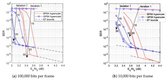
Figure 2.
BER vs. plot for different data frame sizes.
- The simulation BER curves meet the EF bounds, which proves the accuracy of simulation setup and scripts. Moreover, it shows that LABRID is transparent for the overall system performance.
- The position of the turbo cliff for the case of the 10,000 data frame size and QPSK modulation corresponds to its non-LABRID QPSK hypercube BICM-ID reference (Figure 2 in [12]; note the difference in the number of iterations performed and the frame size). It is another proof that LABRID does not deteriorate the overall system performance.
- As expected, the turbo cliff for the longer data frame appears at a lower and is steeper than for the setup with the shorter data frame.
- Particularly for the shorter data frame, there is no real benefit in running as many as 30 decoding iterations (20 are fully enough).
- The EF bound for BPSK hypercube labeling runs significantly lower than for QPSK hypercube labeling and diverges with increasing . It is clear evidence of better asymptotic performance of the former. It agrees with the conclusion ending Section 3.2.
4.2. EXIT Chart Analysis
The EXIT chart [15,16] at for the 4-cube modulations considered in the paper (BPSK, QPSK) is shown in Figure 3. The tunnel between the demapper and decoder transfer curves is opened, so is definitely above the pinch-off limit, regardless of the modulation type considered. It suggests that the simulation BER points should lie on respective modulation-specific EF bounds at the considered , which can be observed exactly in Figure 2a. The transfer curve for the QPSK demapper starts its growth with a higher value of extrinsic mutual information than that for the BPSK demapper, and the tunnel width in its narrowest place is wider for the former than for the latter. It proves faster decoding convergence in the case of the system using QPSK hypercube modulation, which is also reflected in the simulation results at , i.e., the EF bound is met in at most 10 iterations in the case of QPSK, while the system employing BPSK modulation needs more than 20 iterations. On the other hand, the maximal value of the demapper transfer function (observed in the EF case, i.e., at ) is higher in the case of the BPSK demodulator. It gives more reliable decoder a priori LLRs in the final decoding pass, which, in turn, lowers the respective EF bound.
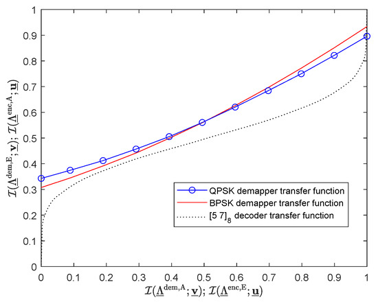
Figure 3.
EXIT chart at ; 100,000 bits per frame.
These conclusions regarding the EXIT tunnel width do not correspond to the plot for the case of the 10,000-bit long data frame, shown in Figure 2b. In detail, at the considered the simulation BER points do not meet the respective EF bounds. So, let us study the reason. The subplots of Figure 4 refer to the following cases: QPSK modulation, 100,000 bits data frame (Figure 4a), QPSK modulation, 10,000 bits (Figure 4b), BPSK modulation, 100,000 bits (Figure 4c), and BPSK modulation, 10,000 bits (Figure 4d). Along with the demapper and decoder transfer curves, they display 10 decoding trajectories exhibiting the lowest demapper a priori mutual information in the last (the 30th) iteration among all transmitted data frames. For the cases where the longer data frame is transmitted (refer to Figure 4a,c), all the considered decoding trajectories tightly match the tunnel created by the transfer curves, so there is neither pdf shape mismatch nor convergence deficiency, and the conclusions based on the EXIT chart observation are fully accurate. On the contrary, if the data frame consists of 10,000 bits (Figure 4b,d), the decoding trajectories visually die out and eventually start to leave the EXIT tunnel, making it impossible to reach the EF range. Since the iterative decoding process cannot converge for at least a few “hopeless” frames, BER increases, substantially. It justifies the gap between the simulation BER curves and their EF bounds at the considered , observed in Figure 2b.
4.3. Efficacy of Frame Filtering
LABRID could be considered a robust solution only if the receivers can efficiently filter out foreign frames. So, the current task is to verify the empirical pdfs of the random variable , representing the absolute extrinsic demapper LLR mean per frame, in two cases: (1) when the receiver obtains the foreign frame, and (2) when it obtains the desired frame. The pdfs shown in Figure 5 are based on the observation of 1000 desired and 1000 foreign frames, both of length 10,000 (such frame length is more realistic than 100,000). In the case of foreign frames, the labeling maps are selected randomly at both the transmitter and receiver sides from the collection of equivalent optimal labelings, and it is guaranteed that they are different from each other. The pdfs are considered in iterations 1...30, separately for QPSK and BPSK hypercube modulation. For better readability, null pdf entries are not shown. Measures are taken at such values of that the simulation BER curves from Figure 5a have just met their respective EF bounds.
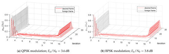
Figure 5.
Growth of the absolute extrinsic demapper LLR mean through subsequent iterations.

Figure 4.
EXIT charts at ; 100,000 bits per frame (a,c) or 10,000 bits per frame (b,d); QPSK modulation (a,b) or BPSK modulation (c,d); the zigzag lines represent the worst 10 decoding trajectories w.r.t. demapper a priori mutual information in the last iteration.
Figure 4.
EXIT charts at ; 100,000 bits per frame (a,c) or 10,000 bits per frame (b,d); QPSK modulation (a,b) or BPSK modulation (c,d); the zigzag lines represent the worst 10 decoding trajectories w.r.t. demapper a priori mutual information in the last iteration.

In both plots it is evident that the absolute extrinsic demapper LLR mean increases in subsequent iterations only if the received frame is the desired frame. Consequently, the pdfs of the two kinds of frames start to disjoint in a few initial iterations, so one can easily classify a given frame as desired or foreign, judging by its value. (As an example, for the QPSK hypercube labeling case considered in Figure 5a, in iteration No. 13 and subsequent, there is no desired frame that exhibits . At the same time, for any foreign frame does not exceed 3, regardless of the iteration number.) It clearly proves that simple threshold-based decisions regarding frame destination can be error-free.
4.4. Desired Threshold Value
The promising results observed in the previous section are specific only to the given considered there. To achieve full success, a more systematic approach is necessary. Therefore, let us measure FAR and MR (defined in Section 2.2) through a whole range of relevant values for arbitrarily chosen threshold values () and for the cases of QPSK and BPSK hypercubes. Our goal is to find a threshold value (constant, if possible) for which both FAR and MR are negligibly small. FAR and MR illustrated by Figure 6 are observed in iteration 20, assuming data frame length of 10,000 (according to Figure 2b, there is no reason for running more decoding passes). In each simulation setup, desired frames and the same number of foreign frames are simulated for statistical reliability reasons.
Figure 6.
FAR and MR vs. vs. threshold applied to the frame filter.
For both considered hypercubes, a massive MR lobe can be observed for low , the occurrence of which results in limited clearance between the MR and FAR surfaces, thereby narrowing the range of optimal values. However, the lobe falls in the same area where the turbo cliff can be found on the respective BER() plots and where BER is usually considered insufficient. Thus, in practice, searching for the optimal threshold value in the turbo cliff region may be pointless.
However, the presence of the lobe does not actually prevent one from setting the optimal threshold for any , as there is still enough room between MR and FAR. In fact, for between, say, 4.0 and 5.0, both MR and FAR are negligibly low in the whole considered range, regardless of the hypercube taken into account.
There is still one more issue to be tackled. In contrast to MR, FAR has the form of a wall that crosses the level of at a value of that gradually grows with increasing . Therefore, eventually (far from the considered ), FAR could appear to be unacceptably high if is fixed. For this reason, the use of low-order modulations with hypercube labeling when is much higher than considered here would require variable . Although such a case is somewhat unrealistic, because a common practice when the channel state improves is to change the modulation order to a higher one, thereby increasing the data rate—in the light of previous contributions [4,5,10] it would also work with LABRID.
4.5. Cost Comparison
The number of different SISO decoder’s operations are specified in Table 3, where is the number of convolutional encoder states, is the number of encoded bits per one trellis segment. The decoder, first, calculates all components for the whole trellis (Step 1). Having obtained them, it can calculate (Step 2) and (Step 3) metrics for all states. Then, it can obtain the extrinsic LLRs related to codeword bits (in all but the last iteration, Step 4a) or the extrinsic LLRs for the data bits (in the last iteration, Step 4b).
Table 3.
Complexity analysis of additive SISO decoder per trellis segment per iteration.
In the last decoding iteration, the decoder (if launched) executes Steps 1–3 and 4b. Then, including the number of trellis segments ( = 10,000), the coding rate , and the number of encoder states (), one obtains additions (or subtractions), multiplications, and max* calculations.
In the case of LABRID, the frame filter calculates the absolute extrinsic demapper LLR mean (it costs additions) and compares it against the threshold (1 regular operation). Division by the number of samples might be omitted if the threshold is set as a higher respective value. The regular decoding steps are executed only for desired frames, and in these cases frame filtering is an additional cost. But for each foreign frame, the receiver avoids running the decoding pass in the last iteration, which is the LABRID advantage. Actually, its efficiency depends on the number of network users, . The maximal number of users in a LABRID system is limited by the number of equivalent labelings (1536 for BPSK/QPSK hypercube labeling, as shown in Section 3.3).
Assuming a genie frame filter mechanism, each frame is classified correctly as a foreign or desired frame (in the light of the results from Section 4.4, the real LABRID receiver introduces just a marginal FAR and MR error in the region of interest). As a consequence, the probability of running the decoding pass in the last iteration is . Figure 7 shows the number of operations executed in the last iteration by the conventional BICM-ID and LABRID receivers. The cost does not include the demapper routine, as it is common for the competing receivers. It can be seen that the computational complexity of the proposed LABRID mechanism declines rapidly with the number of users within a network. The number of the sum of additions and subtractions, asymptotically, meets a floor, which appears due to the need for computation. The number of remaining operations continues to decline linearly on the log-scale with increasing , and even becomes 1000 times lower than the reference BICM-ID in the case of 1536 users of the LABRID network.
Figure 7.
The number of operations of specific type executed in the last decoding pass after generation of the extrinsic demapper LLRs.
Note that the compared costs relate only to the operations in the physical layer. In the case of conservative MAC addressing, every data frame is transferred to the MAC layer, and undergoes integrity checking, which is, literally, another decoding task; it further increases the computational payload for the regular BICM-ID.
5. Conclusions
The concept of hypercube (or multidimensional) labeling has been known for a few years. It helps to overcome the problem of a weak iterative receiver convergence, observed in BICM-ID systems utilizing low-order modulations, such as BPSK or QPSK. In the current paper, another advantage of hypercube labeling has been displayed—the existence of a variety of equivalent optimal labelings which can be used within the framework of the LABRID mechanism to distinguish message recipients within the system. The number of equivalent labelings (more than 1500) is enough to address all stations in most wireless networks.
Since all equivalent labelings exhibit the same distance spectrum, the EF bounds of the LABRID system are identical to those of the regular hypercube BICM-ID system, given modulation order (BPSK or QPSK). In addition, LABRID does not favor any Tx-Rx link over the others in terms of BER for the same reason.
From the analysis of theoretical EF bounds, it is clear that the use of 4-cubes consisting of either four BPSK signals or two QPSK signals leads to a different performance in the considered scenario. Interestingly, the EF bound for the case of a BPSK hypercube lies below that for a QPSK hypercube. This is justified by the fact that the former exploits channel diversity to a higher extent—the signals of the vertex are transmitted within four (not only two) modulation periods, and in each modulation period the channel exhibits another fading gain.
Making decisions on the destination of the frame may rely on a simple threshold crossing rule. The experimental results showed that when the absolute extrinsic demapper LLR mean is checked against a constant threshold, both the false alarm ratio and the misdetection ratio place below , regardless of the considered in the region of interest. The only cost of frame filtering results from the calculation of the mean of (available) absolute extrinsic demapper LLRs. It is incomparably smaller than the price of generating LLRs relative to the data bits in the case of conservative MAC addressing for every foreign frame. LABRID wins the competition in the scenario with just two receivers in a network, but its advantage grows with the number of Rx stations.
Funding
The APC was financed with own funds of the Institute of Radiocommunications, Poznan University of Technology.
Institutional Review Board Statement
Not applicable.
Informed Consent Statement
Not applicable.
Data Availability Statement
Data are contained within the article.
Conflicts of Interest
The author declares no conflict of interest.
References
- Chindapol, A.; Ritcey, J.A. Design, analysis, and performance evaluation for BICM-ID with square QAM constellations in Rayleigh fading channels. IEEE J. Sel. Areas Commun. 2001, 19, 944–957. [Google Scholar] [CrossRef]
- Caire, G.; Taricco, G.; Biglieri, E. Bit-interleaved coded modulation. IEEE Trans. Inf. Theory 1998, 44, 927–946. [Google Scholar] [CrossRef]
- Zehavi, E. 8-PSK trellis codes for a Rayleigh channel. IEEE Trans. Commun. 1992, 40, 873–884. [Google Scholar] [CrossRef]
- Krasicki, M. Labeling-Based Recipient Identification for 16-QAM BICM-ID. EURASIP J. Wirel. Commun. Netw. 2019, 179. [Google Scholar] [CrossRef]
- Krasicki, M. BICM-ID Labeling-Based Recipient Identification in a Heterogeneous Network. Sensors 2023, 23, 3605. [Google Scholar] [CrossRef] [PubMed]
- Zhang, J.; Chen, D.; Wang, Y. A New Constellation Shaping Method and Its Performance Evaluation in BICM-ID. In Proceedings of the 2009 IEEE 70th Vehicular Technology Conference Fall (VTC 2009-Fall), Anchorage, AK, USA, 20–23 September 2009; pp. 1–5. [Google Scholar] [CrossRef]
- Khoo, B.K.; Le Goff, S.; Sharif, B.; Tsimenidis, C. Bit-interleaved coded modulation with iterative decoding using constellation shaping. IEEE Trans. Commun. 2006, 54, 1517–1520. [Google Scholar] [CrossRef][Green Version]
- Basar, E.; Wen, M.; Mesleh, R.; Renzo, M.D.; Xiao, Y.; Haas, H. Index Modulation Techniques for Next-Generation Wireless Networks. IEEE Access 2017, 5, 16693–16746. [Google Scholar] [CrossRef]
- Xu, C.; Xiong, Y.; Ishikawa, N.; Rajashekar, R.; Sugiura, S.; Wang, Z.; Ng, S.X.; Yang, L.L.; Hanzo, L. Space-, Time- and Frequency-Domain Index Modulation for Next-Generation Wireless: A Unified Single-/Multi-Carrier and Single-/Multi-RF MIMO Framework. IEEE Trans. Wirel. Commun. 2021, 20, 3847–3864. [Google Scholar] [CrossRef]
- Krasicki, M. Labeling-Based Recipient Identification for BICM-ID in 64-QAM case. In Proceedings of the 2020 International Wireless Communications and Mobile Computing (IWCMC), Limassol, Cyprus, 15–19 June 2020; pp. 1135–1139. [Google Scholar] [CrossRef]
- Li, X.; Ritcey, J. Trellis-coded modulation with bit interleaving and iterative decoding. IEEE J. Sel. Areas Commun. 1999, 17, 715–724. [Google Scholar] [CrossRef]
- Tran, N.; Nguyen, H. Improving the performance of QPSK BICM-ID by mapping on the hypercube. In Proceedings of the IEEE 60th Vehicular Technology Conference, VTC2004-Fall, Los Angeles, CA, USA, 26–29 September 2004; Volume 2, pp. 1299–1303. [Google Scholar] [CrossRef]
- Tran, N.; Nguyen, H. Design and performance of BICM-ID systems with hypercube constellations. IEEE Trans. Wirel. Commun. 2006, 5, 1169–1179. [Google Scholar] [CrossRef]
- Simoens, F.; Wymeersch, H.; Bruneel, H.; Moeneclaey, M. Multidimensional mapping for bit-interleaved coded modulation with BPSK/QPSK signaling. IEEE Commun. Lett. 2005, 9, 453–455. [Google Scholar] [CrossRef]
- ten Brink, S. Convergence of iterative decoding. Electron. Lett. 1999, 35, 1117–1119. [Google Scholar] [CrossRef]
- Hagenauer, J. The EXIT Chart-Introduction to Extrinsic Information Transfer. In Proceedings of the 12th European Signal Processing Conference (EUSIPCO), Vienna, Austria, 6–10 September 2004; pp. 1541–1548. [Google Scholar]
- Benedetto, S.; Divsalar, D.; Montorsi, G.; Pollara, F. A Soft-Input Soft-Output maximum a posteriori (MAP) module to decode parallel and serial concatenated codes. TDA Prog. Rep. 1996, 42, 1–20. [Google Scholar]
- Robertson, P.; Villebrun, E.; Hoeher, P. A comparison of optimal and sub-optimal MAP decoding algorithms operating in the log domain. In Proceedings of the IEEE International Conference on Communications ICC’95, Seattle, WA, USA, 18–22 June 1995; Volume 2, pp. 1009–1013. [Google Scholar] [CrossRef]
- Land, I.; Hoeher, P.; Gligorevic, S. Computation of symbol-wise mutual information in transmission systems with LogAPP decoders and application to EXIT charts. In Proceedings of the International ITG Conference on Source and Channel Coding, Erlangen, Germany, 14–16 January 2004; pp. 195–202. [Google Scholar]
- Biglieri, E.; Caire, G.; Taricco, G.; Ventura-Traveset, J. Computing error probabilities over fading channels: A unified approach. Eur. Trans. Telecommun. 1998, 9, 15–25. [Google Scholar] [CrossRef]
- Benedetto, S.; Biglieri, E. Principles of Digital Transmission with Wireless Applications; Kluwer Academic Publishers: New York, NY, USA, 1999. [Google Scholar]
- Schreckenbach, F.; Gortz, N.; Hagenauer, J.; Bauch, G. Optimized symbol mappings for Bit-Interleaved Coded Modulation with Iterative Decoding. In Proceedings of the IEEE Global Telecommunications Conference (GLOBECOM’03), San Francisco, CA, USA, 1–5 December 2003; Volume 6, pp. 3316–3320. [Google Scholar] [CrossRef]
- Battiti, R.; Tecchiolli, G. The reactive tabu search. ORSA J. Comput. 1994, 6, 126–140. [Google Scholar] [CrossRef]
- Biglieri, E.; Caire, G.; Taricco, G.; Ventura-Traveset, J. Simple method for evaluating error probabilities. Electron. Lett. 1996, 32, 191–192. [Google Scholar] [CrossRef]


Disclaimer/Publisher’s Note: The statements, opinions and data contained in all publications are solely those of the individual author(s) and contributor(s) and not of MDPI and/or the editor(s). MDPI and/or the editor(s) disclaim responsibility for any injury to people or property resulting from any ideas, methods, instructions or products referred to in the content. |
© 2024 by the author. Licensee MDPI, Basel, Switzerland. This article is an open access article distributed under the terms and conditions of the Creative Commons Attribution (CC BY) license (https://creativecommons.org/licenses/by/4.0/).