

On the Quasistationarity of the Ambient Electromagnetic Field Generated by Wi-Fi Sources


Abstract
1. Introduction
2. Statistical Analysis of RF Signals
2.1. Statistical Indicators of Stationarity and Quasistationarity
2.2. Cumulative Effect and Power Distribution
2.3. Advanced Statistical Assessment of RF Signals
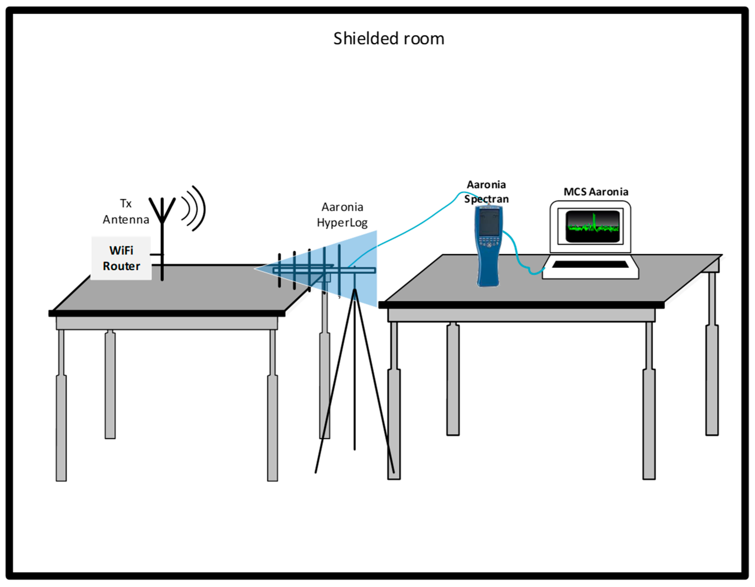
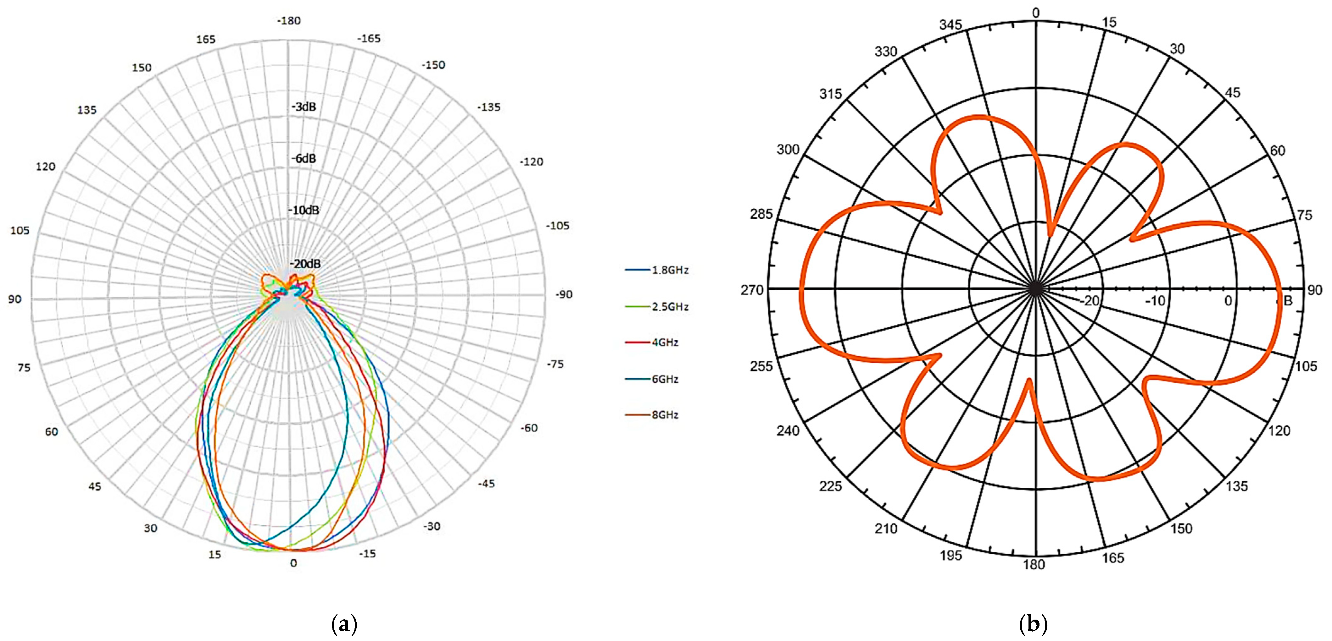
3. Materials and Methods
4. Results
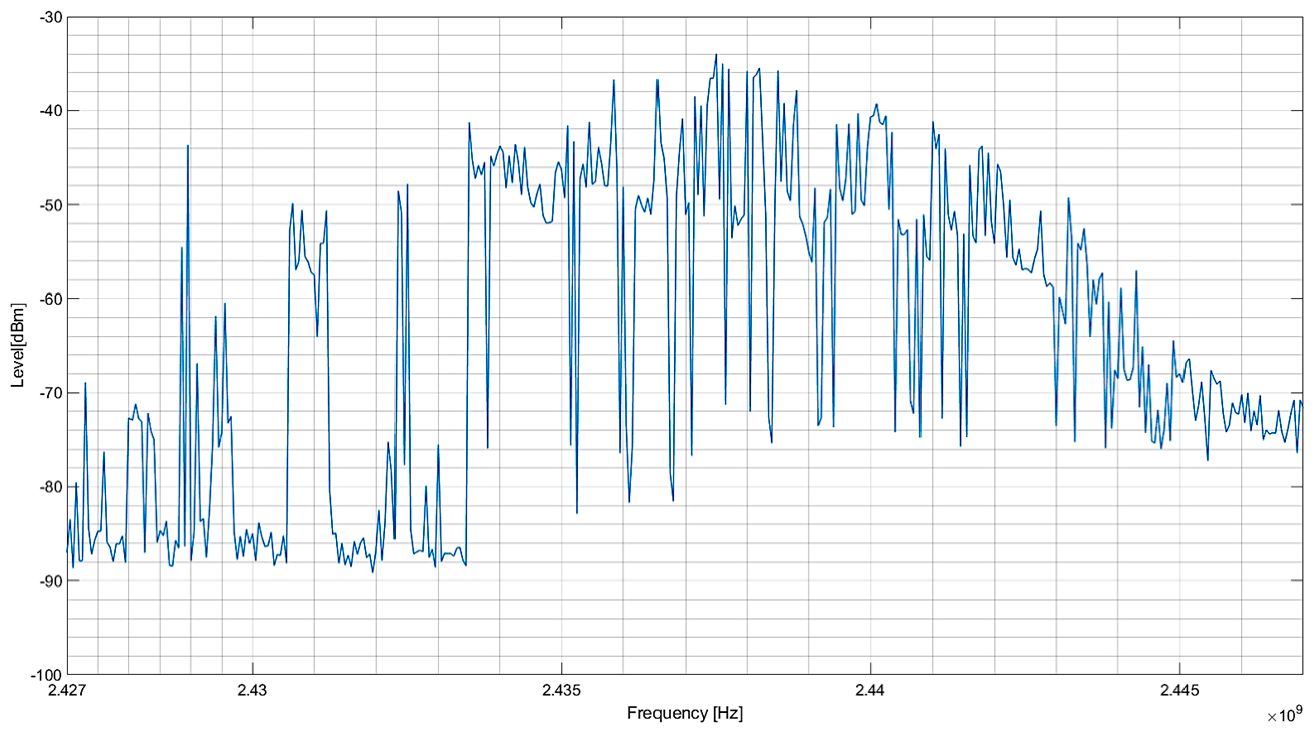
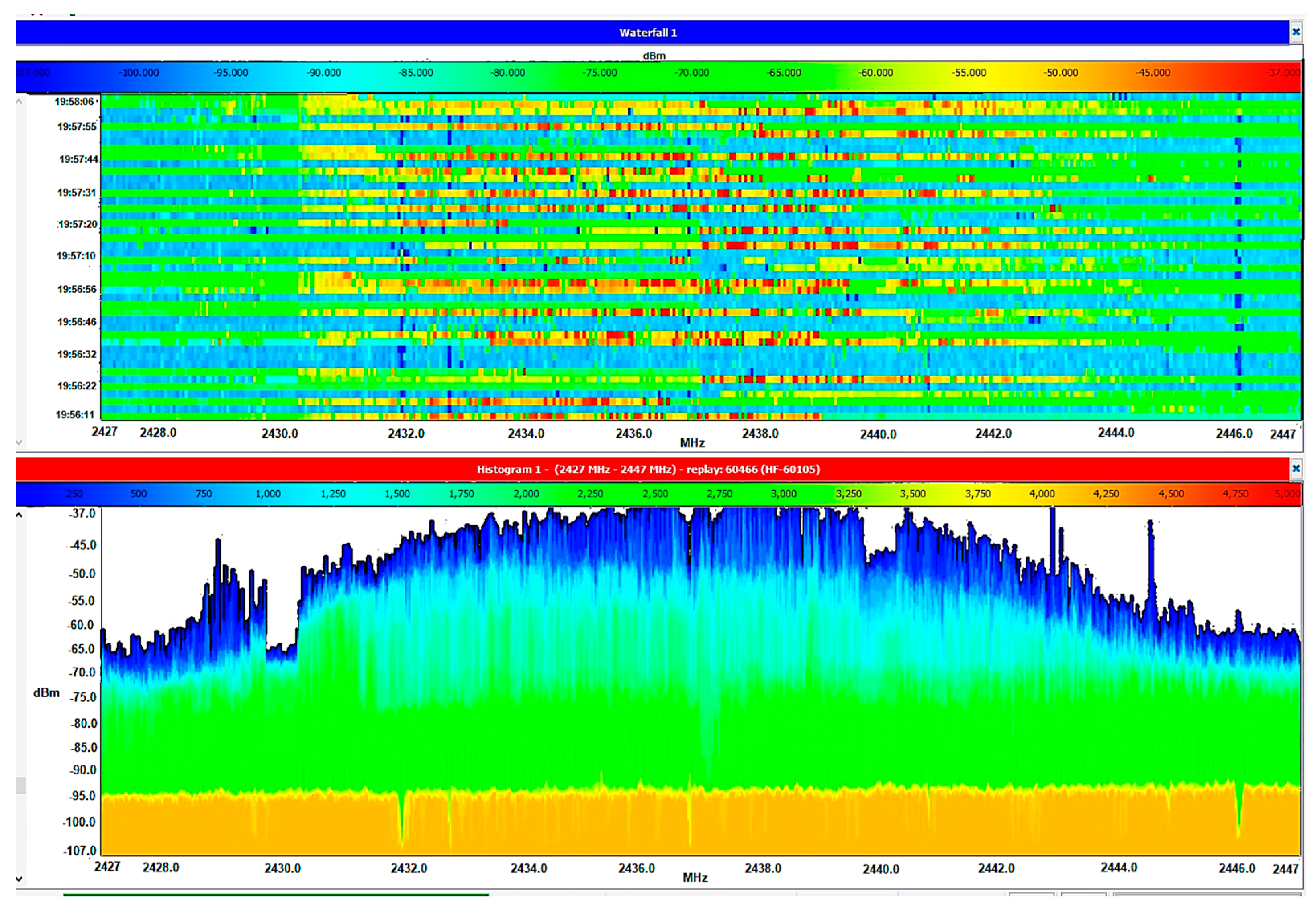
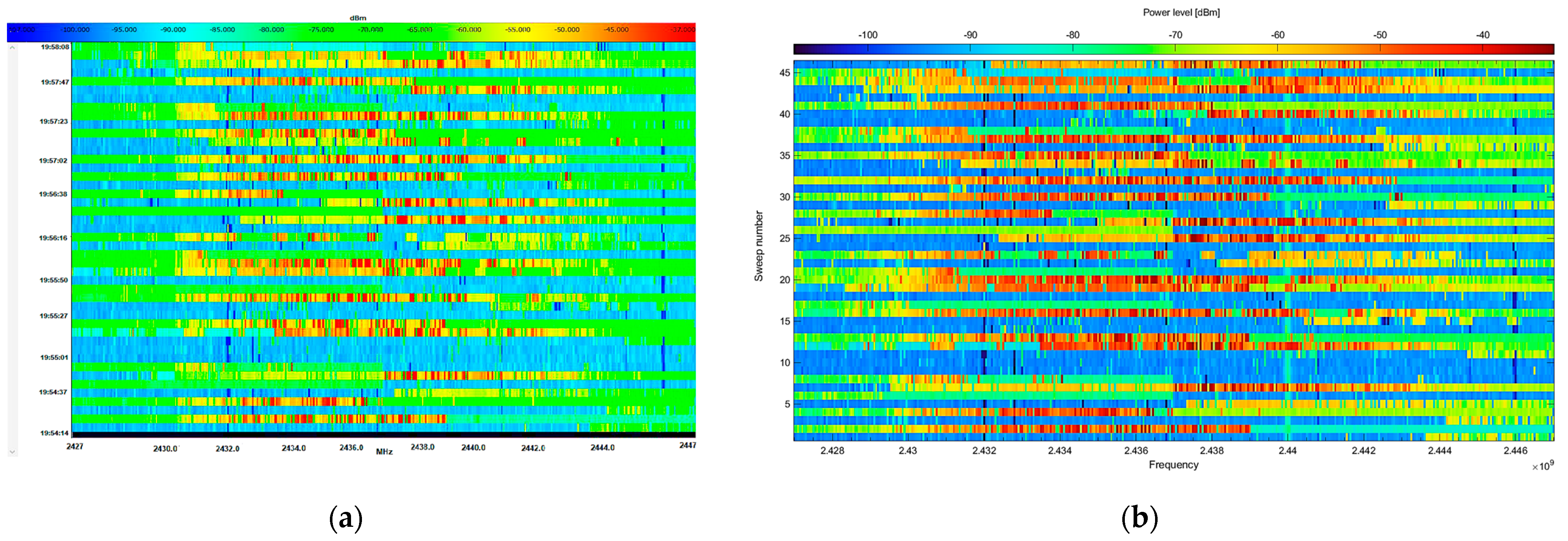
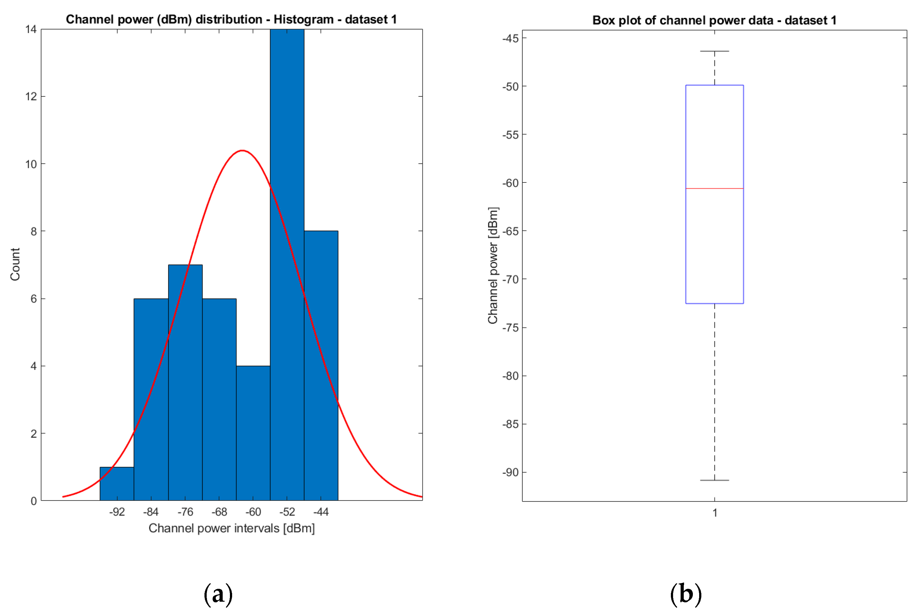
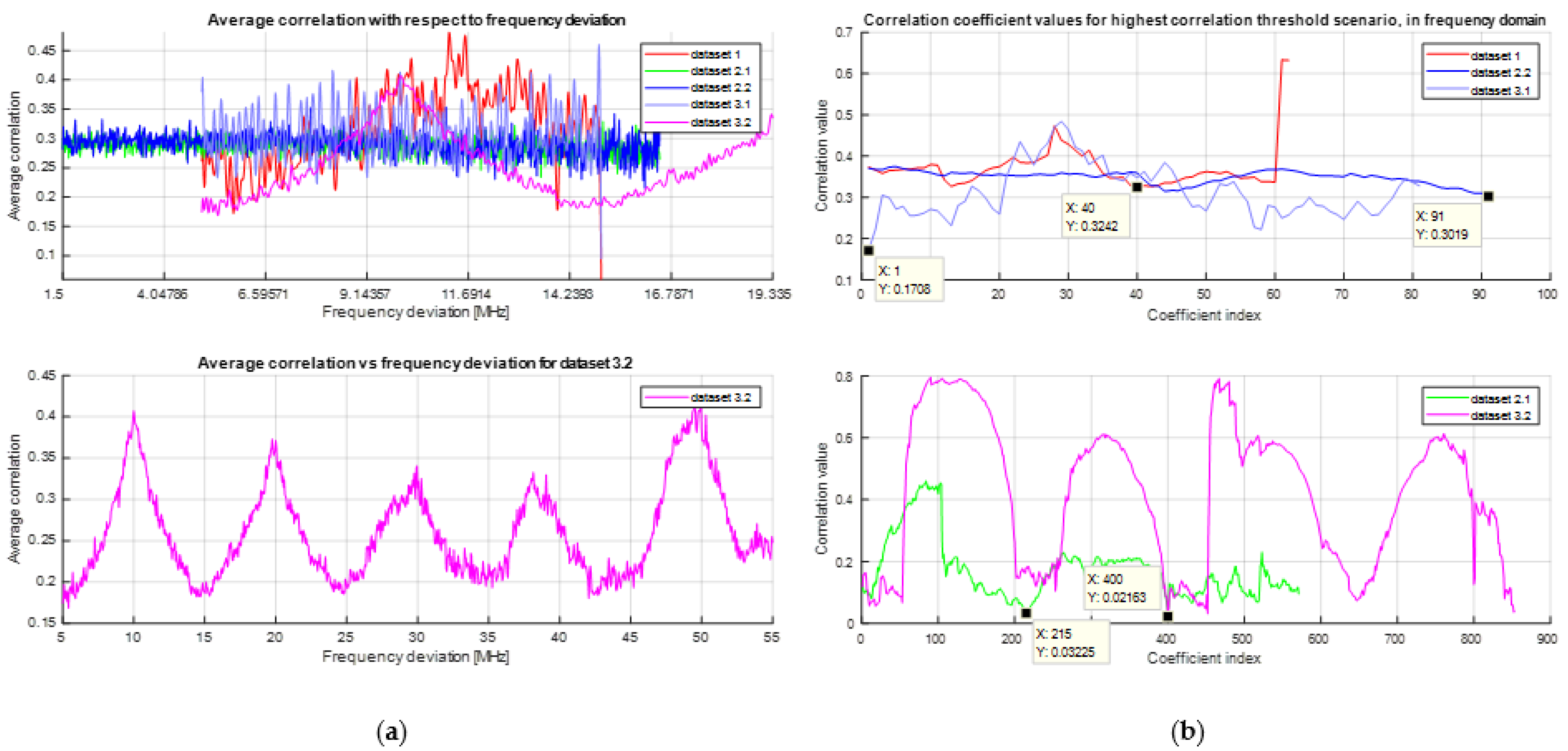
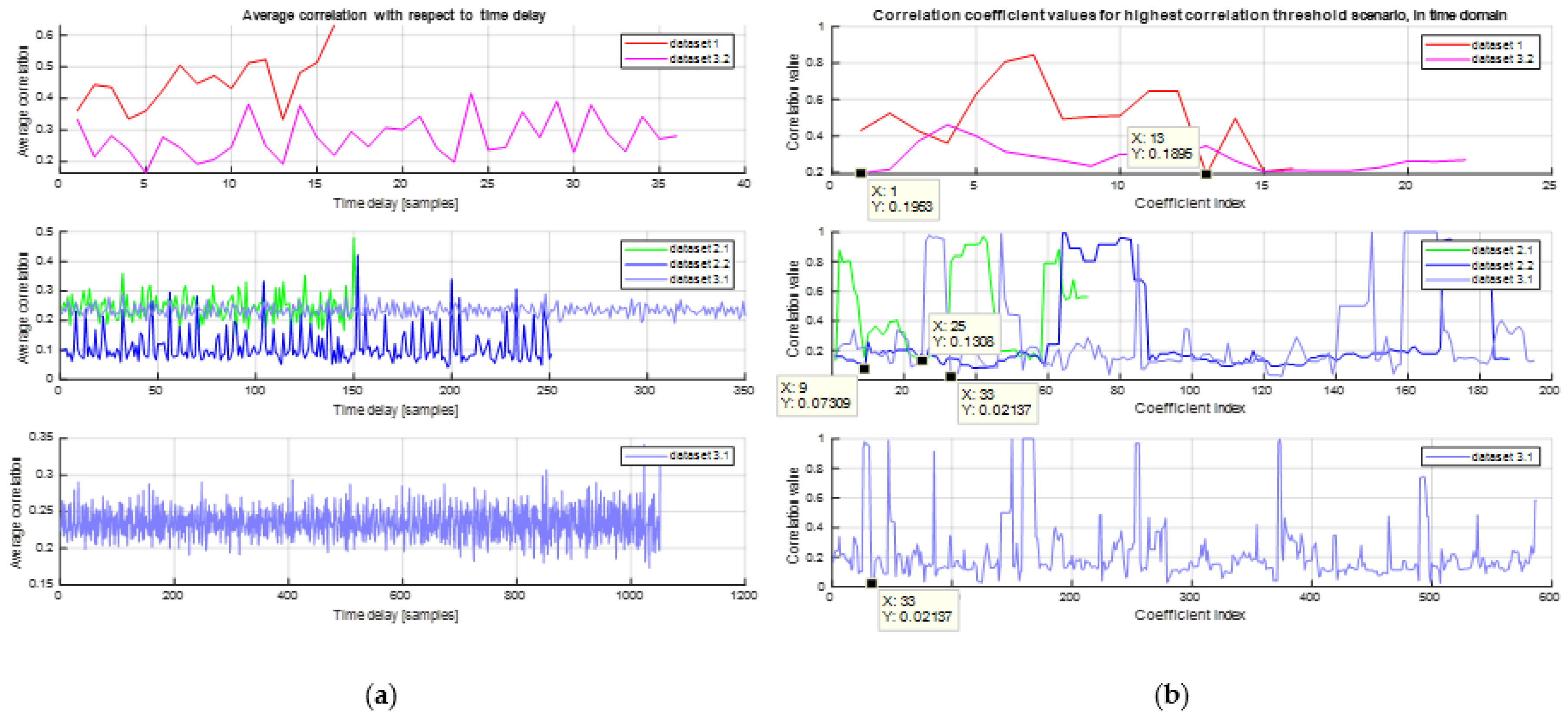
- The initial dataset, denoted as dataset 1, served as the reference for measurements. It was recorded for a brief duration of 2 min while the Wi-Fi source continuously streamed video data on a specific 20 MHz bandwidth channel.
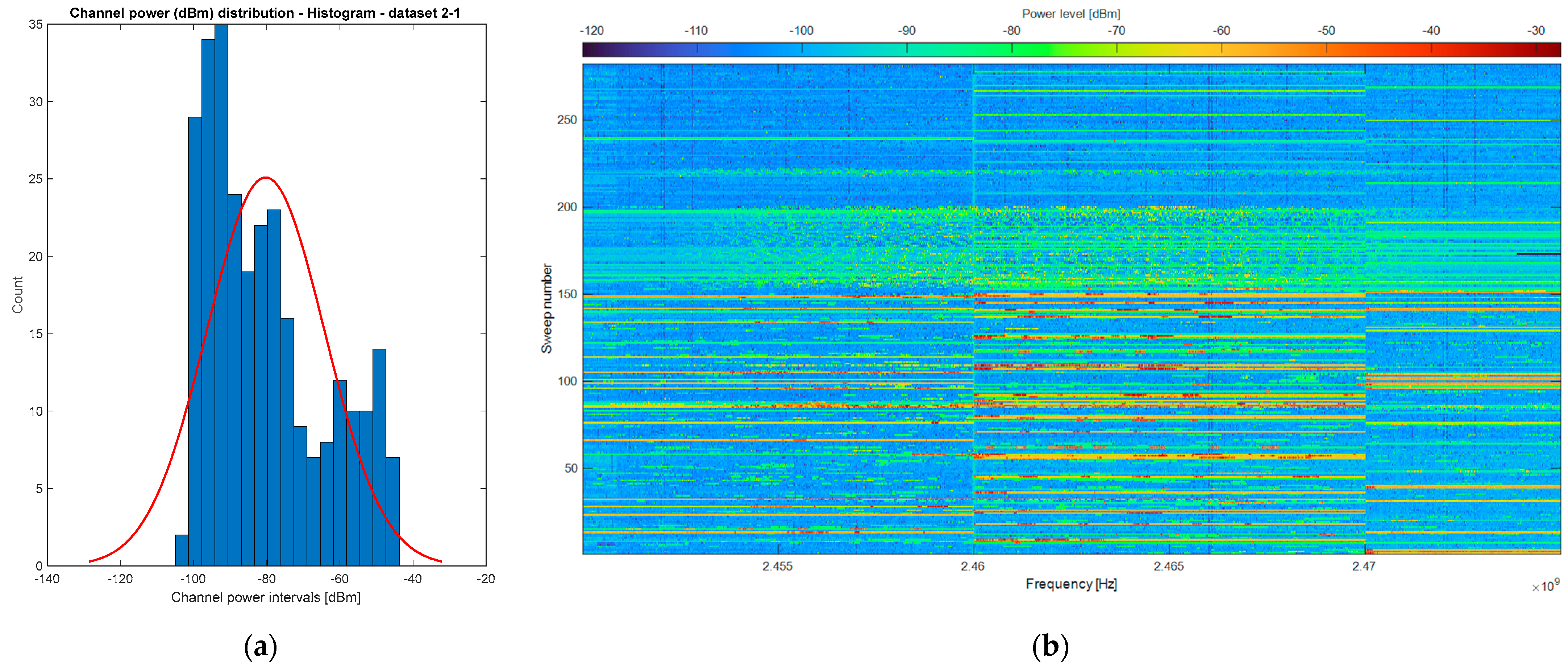
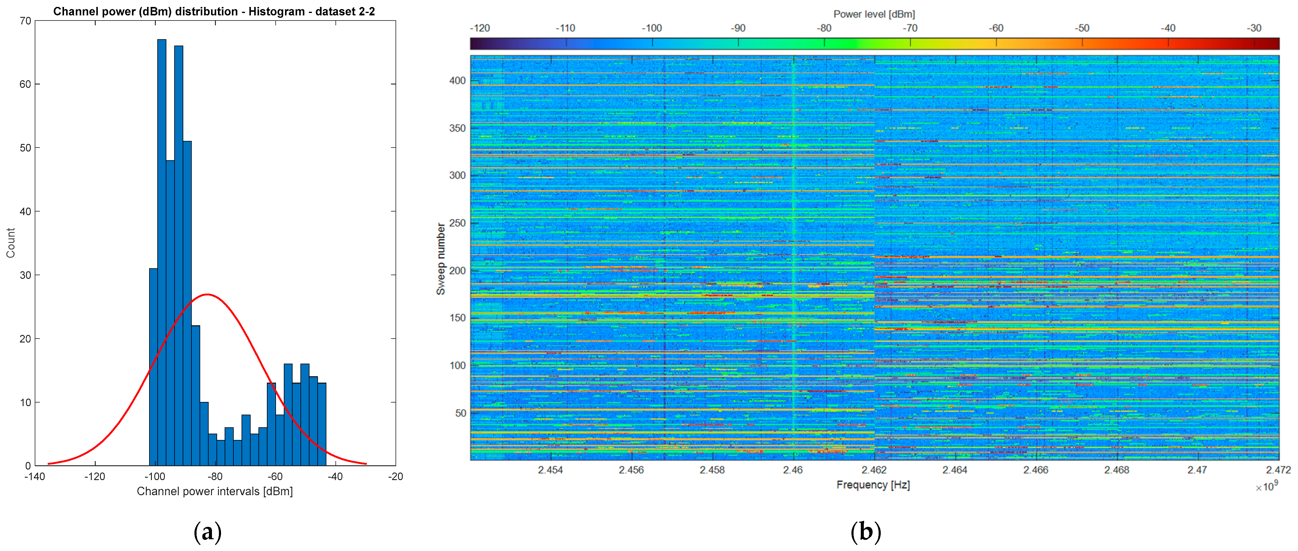
- Datasets 2_1 and 2_2 were captured over an extended time frame of 25 and 30 min, respectively, while maintaining the same bandwidth.
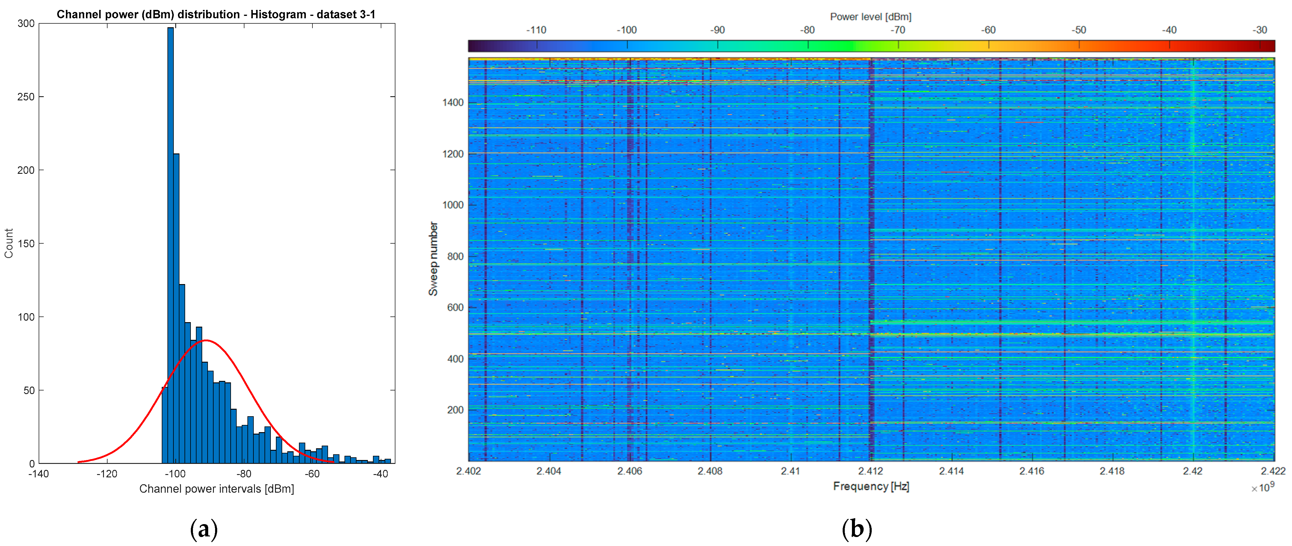
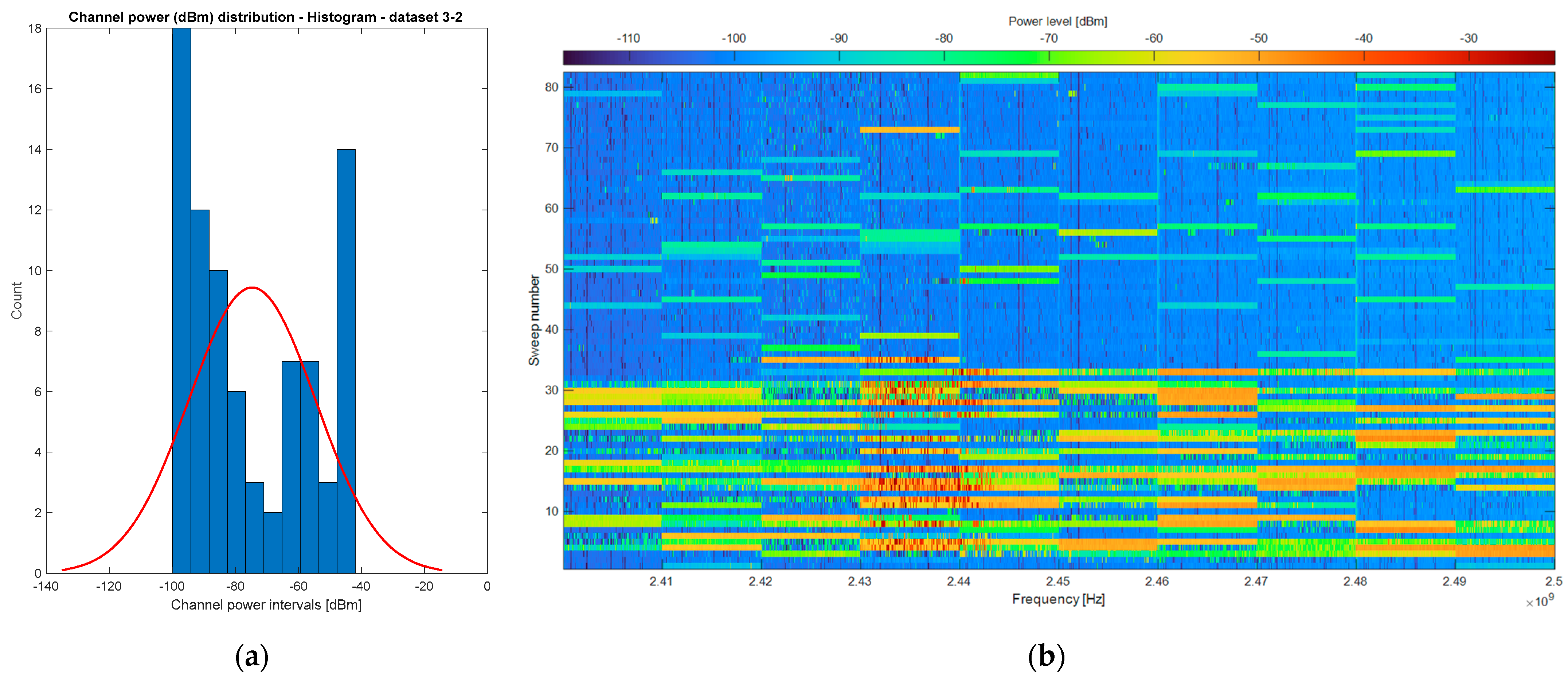
- The third set of measurements resulted in datasets 3_1 and 3_2, expanding the analysis further. Dataset 3_1 had a duration of 60 min, while dataset 3_2 covered an extended frequency band ranging from 2.4 GHz to 2.5 GHz within a constrained temporal duration of 7.5 min.
5. Discussion
6. Conclusions
Author Contributions
Funding
Data Availability Statement
Conflicts of Interest
References
- Gajšek, P.; Ravazzani, P.; Wiart, J.; Grellier, J.; Samaras, T.; Thuróczy, G. Electromagnetic field exposure assessment in Europe radiofrequency fields (10 MHz–6 GHz). J. Expo. Sci. Environ. Epidemiol. 2015, 25, 37–44. [Google Scholar] [CrossRef] [PubMed]
- Atanasova, G.; Atanasov, B.; Atanasov, N. Assessment of Electromagnetic Field Exposure on European Roads: A Comprehensive In Situ Measurement Campaign. Sensors 2023, 23, 6050. [Google Scholar] [CrossRef] [PubMed]
- Urbinello, D.; Joseph, W.; Verloock, L.; Martens, L.; Röösli, M. Temporal trends of radio-frequency electromagnetic field (RF-EMF) exposure in everyday environments across European cities. Environ. Res. 2014, 134, 134–142. [Google Scholar] [CrossRef] [PubMed]
- Sârbu, A.; Miclău, S.; Digulescu, A.; Bechet, P. Comparative Analysis of User Exposure to the Electromagnetic Radiation Emitted by the Fourth and Fifth Generations of Wi-Fi Communication Devices. Int. J. Environ. Res. Public. Health 2020, 17, 8837. [Google Scholar] [CrossRef] [PubMed]
- Mulugeta, B.; Wang, S.; Chikha, W.B.; Liu, J.; Roblin, C.; Wiart, J. Statistical Characterization and Modeling of Indoor RF-EMF Down-Link Exposure. Sensors 2023, 23, 3583. [Google Scholar] [CrossRef] [PubMed]
- Bonato, M.; Dossi, L.; Chiaramello, E.; Fiocchi, S.; Tognola, G.; Parazzini, M. Stochastic Dosimetry Assessment of the Human RF-EMF Exposure to 3D Beamforming Antennas in indoor 5G Networks. Appl. Sci. 2021, 11, 1751. [Google Scholar] [CrossRef]
- European Council. Recommendation of 1999 on the Limitation of Exposure of the General Public to Electromagnetic Fields (0 Hz to 300 GHz). Off. J. Eur. Communities L1999/519/EC 1999, 199, 59–70. [Google Scholar]
- European Union. Directive 2014/30/EU of the European Parliament and of the Council. Off. J. Eur. Union 2014, 96, 79. [Google Scholar]
- Redmayne, M.; Maisch, D. ICNIRP Guidelines’ Exposure Assessment Method for 5G Millimetre Wave Radiation May Trigger Adverse Effects. Int. J. Environ. Res. Public. Health 2023, 20, 5267. [Google Scholar] [CrossRef]
- Chou, C.-K. Controversy in Electromagnetic Safety. Int. J. Environ. Res. Public. Health 2022, 19, 16942. [Google Scholar] [CrossRef]
- Bas, O.; Sengul, I.; Bas, O.; Hanci, H.; Degermenci, M.; Sengul, D.; Altuntas, E.; Soztanaci, U.; Sonmez, O.S.J.J. Impressions of the chronic 900-MHz electromagnetic field in the prenatal period on Purkinje cells in male rat pup cerebella: Is it worth mentioning? Rev. Assoc. Med. Bras. (1992) 2022, 68, 1383–1388. [Google Scholar] [CrossRef] [PubMed]
- Cantürk, T.F.; Yalçin, B.; Yay, A.; Tan, B.; Yeğin, K.; Daşdağ, S. Effects of pre and postnatal 2450 MHz continuous wave (CW) radiofrequency radiation on thymus: Four generation exposure. Electromagn. Biol. Med. 2022, 41, 315–324. [Google Scholar] [CrossRef] [PubMed]
- Er, H.; Tas, G.; Soygur, B.; Ozen, S.; Sati, L. Acute and Chronic Exposure to 900 MHz Radio Frequency Radiation Activates p38/JNK-mediated MAPK Pathway in Rat Testis. Reprod. Sci. 2022, 29, 1471–1485. [Google Scholar] [CrossRef] [PubMed]
- Gupta, S.; Patel, S.; Tomar, M.; Singh, S.; Mesharam, M.; Krishnamurthy, S. Long-term exposure of 2450 MHz electromagnetic radiation induces stress and anxiety like behavior in rats. Neurochem Int. 2019, 128, 1–13. [Google Scholar] [CrossRef] [PubMed]
- National Toxicology Program. NTP TR 596 Technical Report on the Toxicology and Carcinogenesis Studies in B6C3F1/N Mice Exposed to Whole-Body Radio Frequency Radiation at a Frequency (1900 MHz) and Modulations (GSM and CDMA) Used by Cell Phones; U.S. Department of Health and Human Services: Research Triangle Park, NC, USA, 2018.
- Qin, F.; Cao, H.; Yuan, H.; Guo, W.; Pei, H.; Cao, Y.; Tong, J. 1800 MHz radiofrequency fields inhibits testosterone production via CaMKI/RORα pathway. Reprod. Toxicol. 2018, 81, 229–236. [Google Scholar] [CrossRef] [PubMed]
- Rui, G.; Liu, L.; Guo, L.; Xue, Y.; Lai, P.; Gao, P.; Xing, J.; Li, J.; Ding, G. Effects of 5.8 GHz microwave on hippocampal synaptic plasticity of rats. Int. J. Environ. Health Res. 2022, 32, 2247–2259. [Google Scholar] [CrossRef] [PubMed]
- Souffi, S.; Lameth, J.; Gaucher, Q.; Arnaud-Cormos, D.; Lévêque, P.; Edeline, J.-M.; Mallat, M. Exposure to 1800 MHz LTE electromagnetic fields under proinflammatory conditions decreases the response strength and increases the acoustic threshold of auditory cortical neurons. Sci. Rep. 2022, 12, 4063. [Google Scholar] [CrossRef]
- Xue, Y.; Guo, L.; Lin, J.; Lai, P.; Rui, G.; Liu, L.; Huang, R.; Jing, Y.; Wang, F.; Ding, G. Effects of 5.8 GHz Microwaves on Testicular Structure and Function in Rats. BioMed Res. Int. 2022, 2022, 5182172. [Google Scholar] [CrossRef]
- Panagopoulos, D. Analyzing the Health Impacts of Modern Telecommunications Microwaves. In Advances in Medicine and Biology Volume 17; Nova Science Publishers, Inc.: Hauppauge, NY, USA, 2011; pp. 1–55. [Google Scholar]
- Tsatsakis, A.; Kouretas, D.; Tzatzarakis, M.; Stivaktakis, P.; Tsarouhas, K.; Golokhvast, K.; Rakitskii, V.; Tutelyan, V.; Hernandez, A.; Rezaee, R.; et al. Simulating real-life exposures to uncover possible risks to human health: A proposed consensus for a novel methodological approach. Hum. Exp. Toxicol. 2017, 36, 554–564. [Google Scholar] [CrossRef]
- Rowley, J.; Joyner, K. Comparative international analysis of radiofrequency exposure surveys of mobile communication radio base stations. J. Expo. Sci. Environ. Epidemiol. 2012, 22, 304–315. [Google Scholar] [CrossRef]
- Bartosova, K.; Neruda, M.; Vojtech, L. Methodology of Studying Effects of Mobile Phone Radiation on Organisms: Technical Aspects. Int. J. Environ. Res. Public. Health 2021, 18, 12642. [Google Scholar] [CrossRef] [PubMed]
- Kostoff, R.N.; Heroux, P.; Aschner, M.; Tsatsakis, A. Adverse health effects of 5G mobile networking technology under real-life conditions. Toxicol. Lett. 2020, 323, 35–40. [Google Scholar] [CrossRef]
- Sienkiewicz, Z.; Calderón, C.; Broom, K.; Addison, D.; Gavard, A.; Lundberg, L.; Maslanyj, M. Are Exposures to Multiple Frequencies the Key to Future Radiofrequency Research? Front. Public Health 2017, 5, 328. [Google Scholar] [CrossRef] [PubMed]
- Miclaus, S.; Bechet, P.; Iftode, C. The application of a channel-individualized method for assessing long-term, realistic exposure to radiofrequency radiation emitted by mobile communication base station antennas. Measurement 2013, 46, 1355–1362. [Google Scholar] [CrossRef]
- Panagopoulos, D.J.; Johansson, O.; Carlo, G.L. Real versus Simulated Mobile Phone Exposures in Experimental Studies. BioMed Res. Int. 2015, 2015, 607053. [Google Scholar] [CrossRef] [PubMed]
- Modell, H.; Cliff, W.; Michael, J.; McFarland, J.; Wenderoth, M.; Wright, A. A physiologist’s view of homeostasis. Adv. Physiol. Educ. 2015, 39, 259–266. [Google Scholar] [CrossRef] [PubMed]
- Vodovotz, Y.; An, G.; Androulakis, I. A systems engineering perspective on homeostasis and disease. Front. Bioeng. Biotechnol. 2013, 1, 6. [Google Scholar] [CrossRef]
- Roşu, G.; Spandole-Dinu, S.; Catrina, A.-M.; Tuţă, L.; Baltag, O.; Fichte, L.-O. On the adapting ability of living organisms to stationary and non-stationary electromagnetic fields. IOP Conf. Ser. Mater. Sci. Eng. 2022, 1254, 012024. [Google Scholar] [CrossRef]
- Rust, H. Spectral Analysis of Stochastic Processes; E2C2/GIACS Summer School: Comorova, Romania, 2007. [Google Scholar]
- IEEE-SA. The Evolution of Wi-Fi Technology and Standards. 16 May 2023. Available online: https://standards.ieee.org/beyond-standards/the-evolution-of-wi-fi-technology-and-standards/ (accessed on 10 November 2023).
- Papoulis, A.; Pillai, S.U. Probability, Random Variables, and Stochastic Processes; McGraw-Hill Higher Education: New York, NY, USA, 2002. [Google Scholar]
- Tan, Y.; Wang, C.-X.; Nielsen, J.Ø.; Pedersen, G.F. Comparison of stationarity regions for wireless channels from 2 GHz to 30 GHz. In Proceedings of the 2017 13th International Wireless Communications and Mobile Computing Conference (IWCMC), Valencia, Spain, 26–30 June 2017; pp. 647–652. [Google Scholar] [CrossRef]
- Spandole-Dinu, S.; Catrina, A.-M.; Voinea, O.; Andone, A.; Radu, S.; Haidoiu, C.; Călborean, O.; Popescu, D.; Suhăianu, V.; Baltag, O.; et al. Pilot Study of the Long-Term Effects of Radiofrequency Electromagnetic Radiation Exposure on the Mouse Brain. Int. J. Environ. Res. Public. Health 2023, 20, 3025. [Google Scholar] [CrossRef]
- IEEE Computer Society. IEEE Std 802.11™ IEEE Standard for Information Technology, Part 11: Wireless LAN Medium Access Control; The Institute of Electrical and Electronics Engineers: New York, NY, USA, 2021; ISBN 9781504472838/9781504472845. [Google Scholar]
- Banerji, S.; Chowdhury, R.S. On IEEE 802.11: Wireless LAN Technology. Int. J. Mob. Netw. Commun. Telemat. (IJMNCT) 2013, 3, 45–64. [Google Scholar] [CrossRef]
- Tardioli, D.; Almeida, L. Behavior of IEEE 802.11 devices under interference. In Proceedings of the IEEE 28th International Conference on Emerging Technologies and Factory Automation (ETFA), Sinaia, Romania, 12–15 September 2023. [Google Scholar] [CrossRef]
- Kostuch, A.; Gierłowski, K.; Wozniak, J. Performance Analysis of Multicast Video Streaming in IEEE 802.11 b/g/n Testbed Environment. In Proceedings of the IFIP International Federation for Information Processing, Gdańsk, Poland, 9–11 September 2009; pp. 92–105. [Google Scholar]
- Rosu, G.; Tuta, L.; Halca, A.; Bicheru, S.; Hertzog, R.; Baltag, O. Experimental Platform for Studying the Impact of Environ-mental Electromagnetic Fields on Living Organisms. In Proceedings of the 13th International Conference on Communications (COMM), Bucharest, Romania, 18–20 June 2020. [Google Scholar]
- Narasimhamurthy, A.B.; Banavar, M.K.; Tepedelenlioğlu, C. Peak to Average Power Ratio. In OFDM Systems for Wireless Communications; Springer Nature: Cham, Switzerland, 2010; pp. 31–32. [Google Scholar]
- Pisa, S.; Pittella, E.; Piuzzi, E. A survey of radar systems for medical applications. IEEE Aerosp. Electron. Syst. Mag. 2016, 31, 64–81. [Google Scholar] [CrossRef]
- Joseph, W.; Pareit, D.; Vermeeren, G.; Naudts, D.; Verloock, L.; Martens, L.; Moerman, I. Determination of the duty cycle of WLAN for realistic radio frequency electromagnetic field exposure assessment. Prog. Biophys. Mol. Biology. 2013, 111, 30–36. [Google Scholar] [CrossRef] [PubMed]
- Technologies, A. Characterizing Digitally Modulated Signals with CCDF Curves. Application Note; Agilent Technologies: Santa Clara, CA, USA, 2000. [Google Scholar]
- Champagnat, N.; Villemonais, D. General criteria for the study of quasi-stationarity. Electron. J. Probab. 2023, 28, 1–84. [Google Scholar] [CrossRef]
- Sunao, R.; Satoru, A. Development of Multi-channel APD (Amplitude Probability Distribution) Measuring Apparatus. Anritsu Tech. Rev. 2013, 20, 42–52. [Google Scholar]
- Stoica, P.; Moses, R. Spectral Analysis of Signals; Prentice Hall: Hoboken, NJ, USA, 2005. [Google Scholar]
- Tognola, G.; Plets, D.; Chiaramello, E.; Gallucci, S.; Bonato, M.; Fiocchi, S.; Parazzini, M.; Martens, L.; Joseph, W.; Ravazzani, P. Use of Machine Learning for the Estimation of Down- and Up-Link Field Exposure in Multi-Source Indoor WiFi Scenarios. Bioelectromagnetics 2021, 42, 550–561. [Google Scholar] [CrossRef] [PubMed]
- Rauscher, C. Fundamentals of Spectrum Analysis; Rohde & Schwarz GmbH: München, Germany, 2001. [Google Scholar]
- Miclaus, S.; Deaconescu, D.; Vatamanu, D.; Buda, A. An Exposimetric Electromagnetic Comparison of Mobile Phone Emissions: 5G versus 4G Signals Analyses by Means of Statistics and Convolutional Neural Networks Classification. Technologies 2023, 11, 113. [Google Scholar] [CrossRef]


| Dataset | Parameters | Channel Power (CP) Descriptive Statistics | ||||
|---|---|---|---|---|---|---|
| Bandwidth | Duration | Mean [dBm] | Standard Deviation [dBm] | Skewness | Kurtosis | |
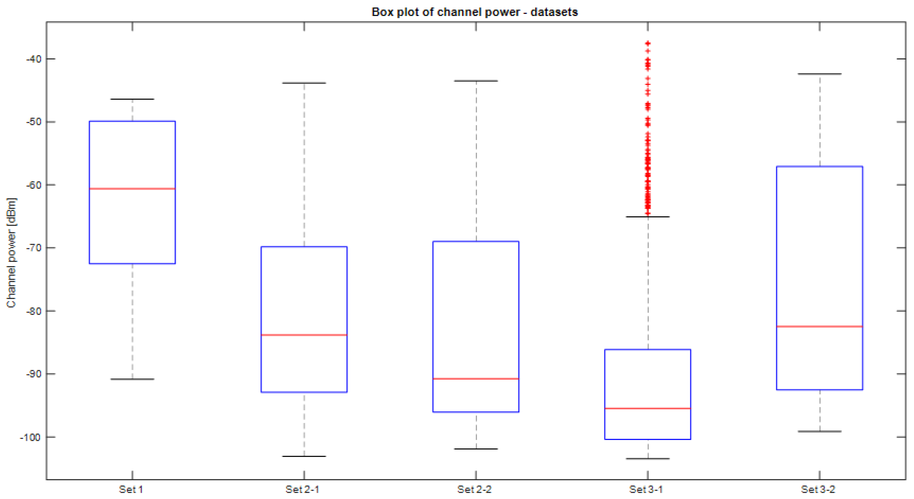
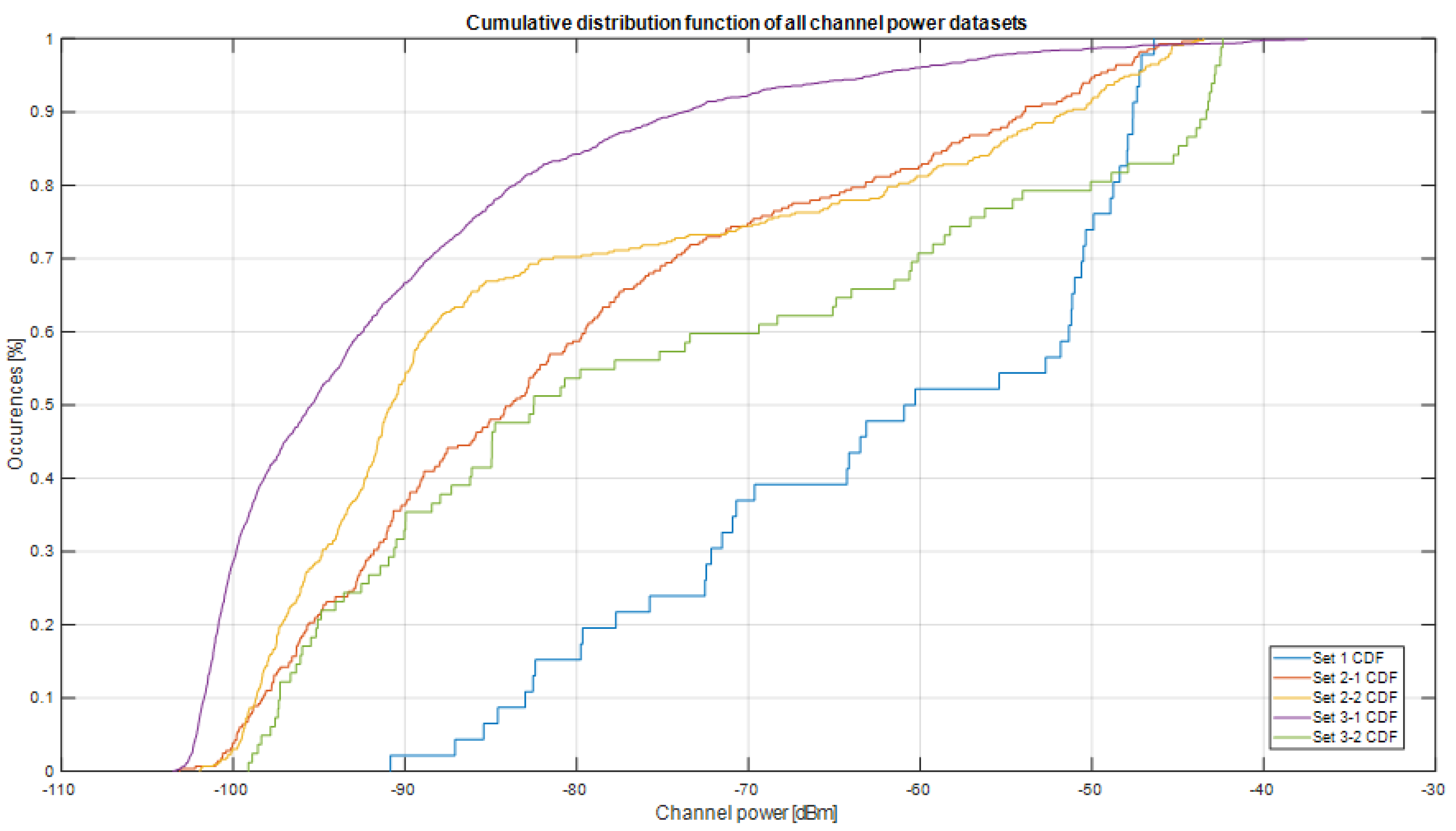
| 1 | 20 MHz | 2 min | −62.5238 | 14.1263 | −0.4333 | 1.7261 |
| 2_1 | 20 MHz | 25 min | −80.3227 | 16.0795 | 0.6711 | 2.2847 |
| 2_2 | 20 MHz | 30 min | −82.7335 | 17.6729 | 0.9765 | 2.4174 |
| 3_1 | 20 MHz | 60 min | −91.1383 | 12.4992 | 1.6836 | 5.7821 |
| 3_2 | 100 MHz | 7.5 min | −74.7298 | 20.1055 | 0.4105 | 1.6322 |
| Dataset | Frequency | Time | ||||
|---|---|---|---|---|---|---|
| Allowance of Similarity Level | Highest Correlation Average | Average Correlation (for All Δf and Sliding Window Sizes) | Allowance of Similarity Level | Highest Correlation Average | Average Correlation (for All Δt and Sliding Window Sizes) | |
| 1 | 0.32 | 0.4728 | 0.2728 | 0.18 | 0.6311 | 0.3889 |
| 2-1 | 0.03 | 0.3289 | 0.1628 | 0.13 | 0.4795 | 0.1507 |
| 2-2 | 0.3 | 0.3537 | 0.2 | 0.07 | 0.4208 | 0.1430 |
| 3-1 | 0.17 | 0.4101 | 0.2243 | 0.02 | 0.3421 | 0.0686 |
| 3-2 | 0.03 | 0.5525 | 0.2228 | 0.19 | 0.4165 | 0.2429 |
| Dataset | Frequency | Time | ||
|---|---|---|---|---|
| Frequency Deviation Δf/Stationary Bandwidth [MHz] | Sliding Window Size [MHz] | Time Delay Δt/Stationary Interval [s] | Sliding Window Size [s] | |
| 1 | 14.55 | 2.35 | 63.6 | 13.25 |
| 2-1 | 14.205 | 2.22 | 1055.3 | 63.96 |
| 2-2 | 16.395 | 2.235 | 954.24 | 55.38 |
| 3-1 | 13.5 | 2.45 | 1114.9 | 10.26 |
| 3-2 | 50.35 | 9.65 | 275.87 | 56.3 |
| Dataset | Mean | Variance | Skewness | Kurtosis |
|---|---|---|---|---|
| 1 | 9.6532 × 10⁻⁴ | 4.6564 × 10⁻⁶ | 1.9185 | 6.8177 |
| 2.1 | 2.0697 × 10⁻⁴ | 1.5282 × 10⁻⁶ | 7.3206 | 70.4443 |
| 2.2 | 2.4991 × 10⁻⁴ | 2.1950 × 10⁻⁶ | 8.3283 | 96.3299 |
| 3.1 | 8.9638 × 10⁻⁵ | 9.3443 × 10⁻⁷ | 15.8252 | 300.1463 |
| 3.2 | 4.8693 × 10⁻⁴ | 8.0357 × 10⁻⁶ | 3.3214 | 13.8578 |
| Average | 3.9975 × 10⁻⁴ | 3.4699 × 10⁻⁶ | 7.3428 | 97.5192 |
| Simulated Wi-Fi Dataset | 1 | 2 | 3 | 4 | 5 | 6 | 7 | 8 | 9 | 10 |
|---|---|---|---|---|---|---|---|---|---|---|
| Mean | 3.9975 × 10⁻⁴ | |||||||||
| Variance | 3.4699 × 10⁻⁶ | |||||||||
| Skewness | 7.5140 | 7.4710 | 7.6260 | 7.6960 | 7.6733 | 7.6472 | 7.6631 | 7.6854 | 7.7020 | 7.5881 |
| Kurtosis | 102.1945 | 92.7767 | 95.6092 | 94.2125 | 98.4178 | 97.9201 | 93.5759 | 93.8203 | 95.6573 | 92.6714 |
| Allowance of similarity level | 0.12 | 0.10 | 0.09 | 0.07 | 0.09 | 0.09 | 0.08 | 0.08 | 0.08 | 0.08 |
| Highest correlation average | 0.3724 | 0.3759 | 0.3473 | 0.3553 | 0.3460 | 0.3587 | 0.3295 | 0.3785 | 0.3510 | 0.3507 |
| Average correlation | 0.1160 | 0.1109 | 0.1125 | 0.1110 | 0.1138 | 0.1151 | 0.1130 | 0.1102 | 0.1110 | 0.1116 |
Disclaimer/Publisher’s Note: The statements, opinions and data contained in all publications are solely those of the individual author(s) and contributor(s) and not of MDPI and/or the editor(s). MDPI and/or the editor(s) disclaim responsibility for any injury to people or property resulting from any ideas, methods, instructions or products referred to in the content. |
© 2024 by the authors. Licensee MDPI, Basel, Switzerland. This article is an open access article distributed under the terms and conditions of the Creative Commons Attribution (CC BY) license (https://creativecommons.org/licenses/by/4.0/).
Share and Cite
Tuță, L.; Roșu, G.; Andone, A.; Spandole-Dinu, S.; Fichte, L.O. On the Quasistationarity of the Ambient Electromagnetic Field Generated by Wi-Fi Sources. Electronics 2024, 13, 301. https://doi.org/10.3390/electronics13020301
Tuță L, Roșu G, Andone A, Spandole-Dinu S, Fichte LO. On the Quasistationarity of the Ambient Electromagnetic Field Generated by Wi-Fi Sources. Electronics. 2024; 13(2):301. https://doi.org/10.3390/electronics13020301
Chicago/Turabian StyleTuță, Leontin, Georgiana Roșu, Alina Andone, Sonia Spandole-Dinu, and Lars Ole Fichte. 2024. "On the Quasistationarity of the Ambient Electromagnetic Field Generated by Wi-Fi Sources" Electronics 13, no. 2: 301. https://doi.org/10.3390/electronics13020301
APA StyleTuță, L., Roșu, G., Andone, A., Spandole-Dinu, S., & Fichte, L. O. (2024). On the Quasistationarity of the Ambient Electromagnetic Field Generated by Wi-Fi Sources. Electronics, 13(2), 301. https://doi.org/10.3390/electronics13020301