SDR-Based Portable System for Evaluating Exposure to Ambient Electromagnetic Fields

Abstract

This paper discusses the need to accurately determine the population’s exposure to low-intensity radio-frequency electromagnetic fields (RF-EMF) from modern technologies like mobile networks, Wi-Fi, and IoT and proposes a practical solution for this assessment. There is no scientific consensus on the biological effects, mostly due to challenges in conducting accurate biological experiments. Recent research suggests that real-life exposure sources trigger stronger biological responses than laboratory-generated RF-EMF. However, there is a lack of research comparing the effects of these sources. This paper introduces a portable system for assessing and monitoring EMF exposure in urban areas. Employing a Software-Defined Radio (SDR) platform to ensure adaptability, the system incorporates two measurement configurations. The initial version concentrates on determining the average power within a 20 MHz Wi-Fi channel, whereas the subsequent configuration augments its functionality by introducing a frequency sweep. This sweep broadens the scrutinized bandwidth, thereby enriching the captured data content through the storage of spectrum sweeps corresponding to each average power value. These data can be used to create EMF profile maps based on individuals’ geographical coordinates. Compared to current limited-performance commercial exposimeters, the proposed system offers expanded capabilities by broadening the frequency bandwidth, georeferencing measurements, and storing data in an SQL database. Compared to high-performance commercial exposimeters, the major advantage of the system is its ability to detect short-term fluctuations in signal spectra and store the corresponding data for subsequent analysis.

1. Introduction

The persistent exposure of the population to low-intensity RF-EMF is a fact and primarily stems from the widespread use of mobile communication networks, Wi-Fi, and the more recent Internet of Things (IoT) network. The issue of biological effects of this exposure, however, lacks scientific consensus, primarily due to the difficulty in organizing both accurate and relevant biological experiments, leading to conflicting scientific findings [1,2]. Furthermore, the scientific community investigating these biological effects faces difficulties in keeping pace with the rapid evolution of emerging technologies [3,4]. Additionally, there is substantial variability in the experimental conditions employed for in vivo studies [5].

While most experiments employ laboratory equipment as RF-EMF generators with fixed or slowly changing parameters, recent research indicates that employing actual “real-life” exposure sources elicits more pronounced biological responses [6]. The translation of findings from controlled experiments to real-life exposure scenarios presents challenges, not exclusive to RF-EMF exposure [7]. Contemporary methodologies for estimating real-life exposure even involve the utilization of machine learning algorithms [8]. Nonetheless, there is a deficiency in research comparing the biological effects of laboratory-generated RF-EMF with those from real-life sources [6,9,10].

Urban environments, in particular, have experienced a proliferation of numerous radio transmitters, resulting in the establishment of a continuously changing multispectral RF environment. This environment exposes the broader population to electromagnetic waves of low intensity, characterized by fluctuations in intensity, polarization, and frequency content. Numerous research studies have tackled the assessment of temporal or spatial variations in exposure to ambient electromagnetic fields [11,12,13,14,15]. These investigations involve conducting measurement campaigns in diverse locations and micro-environments, encompassing both indoor and outdoor settings.

In Europe, for example, 2G, 3G, and 4G cellular networks operate concurrently, with some regions also utilizing 5G technology. These networks provide voice and data services, and a significant portion of users—approximately 80%—are located indoors while the base station is typically situated outside. Telecommunications engineers strive to achieve comprehensive network coverage, including indoor areas, but this objective leads to the quasi-permanent presence of low-intensity RF-EMF indoors. Characterizing exposure levels in indoor environments proves to be a more straightforward task, primarily relying on the utilization of fixed laboratory equipment powered by an electrical network [3,8,16,17].

The field of exposimetric portable sensors for evaluating electromagnetic pollution at an individual level is an emerging and evolving area of research. Currently, the research is focused on the development of narrow-band sensors [18]. Most restricted-capability solutions have limitations concerning frequency bandwidths and lack correlation between the measured field data and the geographic position of the measurements [19,20] or are limited to indoor environments [21]. Even currently available advanced-performance commercial exposimeters that include these options have a major limitation in their inability to detect short-term fluctuations in signal spectra [22].

This paper presents a versatile solution for an enhanced portable system designed for the assessment and monitoring of human exposure to EMFs within densely populated urban settings. The core of this system utilizes a budget-friendly SDR platform, which imbues it with a remarkable degree of versatility concerning the nature of the output data it can produce. The combined cost of the system components, including the HackRF SDR and the Raspberry Pi processing unit, is below EUR 500. The novelty of the proposed system lies in its expanded capabilities relative to conventional exposimeters available in the commercial market, which predominantly rely on narrow-band sensors. This extension is achieved by harnessing the potential of SDR technology to broaden the frequency bandwidth and the possibility to detect short-term fluctuations in signal spectra. Additionally, the system incorporates georeferencing of field measurements and storage of the measurement data in a Structured Query Language (SQL) database. The database can then be used to create an EMF profile map that is contingent upon the geographical coordinates of individuals wearing specific sensors.

2. Materials and Methods

This section describes the steps undertaken in the design of the EMF exposure measurement system, represented by a block diagram depicted in Figure 1. As noted, the RF-EMF measurement unit consists in a low-cost SDR HackRF and an omnidirectional receiving antenna. The system’s core unit is represented by a Raspberry Pi 400 platform, which is basically a programmable computer based on the Advanced RISC Machine (ARM) architecture and runs on the Linux-based Raspberry Pi operating system (OS) also known as Raspbian. The Raspberry Pi 400 is designed in the form of a compact keyboard, with the computer components integrated into the keyboard itself.

Figure 1 highlights the process by which information contained within a signal spectrum is conveyed for subsequent processing through GNU Radio software 3.7.13.5. This is succeeded by data acquisition through a Python application and its subsequent storage within a PostgreSQL database, accompanied by concurrent recording of Global Positioning System (GPS) coordinates. Furthermore, the system incorporates georeferencing metadata and collates real-time average power metrics specific to a designated Wi-Fi channel within the database.

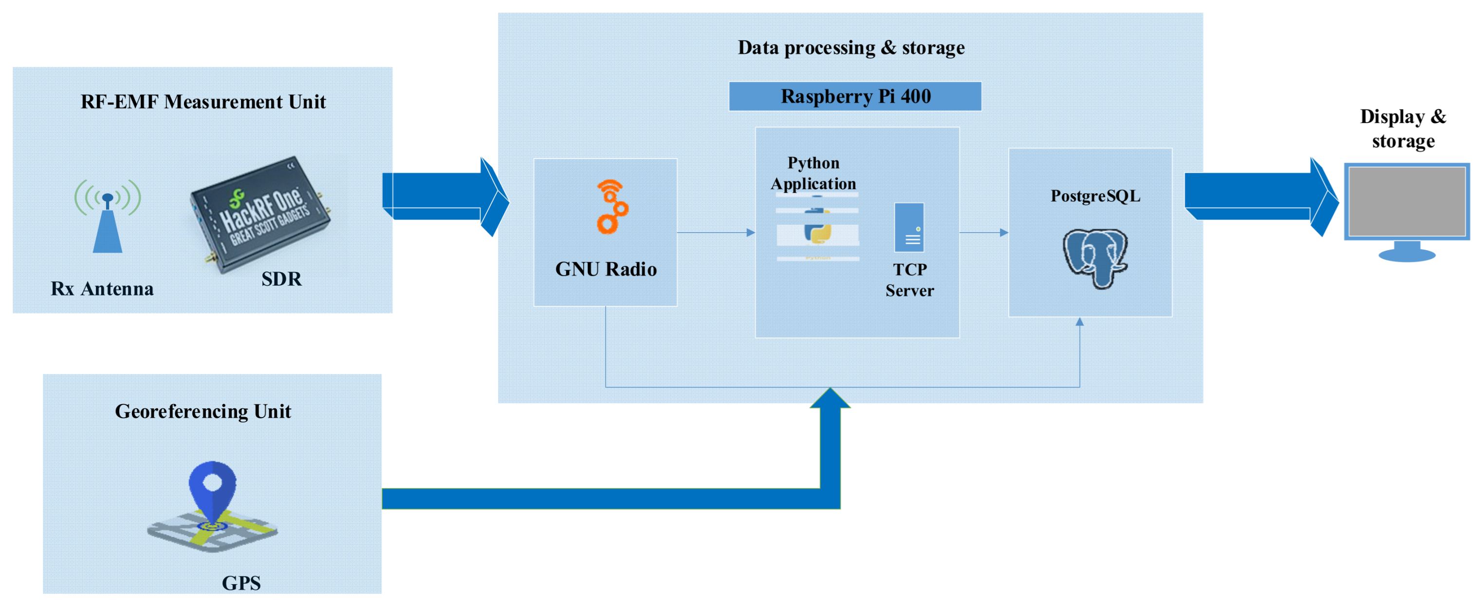
2.1. RF-EMF Measurement Unit Design

The RF-EMF measurement unit, using the highly versatile SDR device HackRF, has the capability to receive radio signals in the frequency range of 1 MHz to 6 GHz. The SDR device relies on the Cypress FX3 USB 3.0 SuperSpeed controller, with a Digital Signal Processing (DSP) component with a high data processing capacity. The SDR system is also equipped with RF filters, amplifiers, and oscillators, which exhibit exceptional performance and signal quality attributes [22]. In contrast to traditional receivers, the signal processing workflow of the SDR entails the following stages subsequent to the traditional intermediate-frequency (IF) demodulation: Firstly, the analog IF signal is directed to an Analog-to-Digital Converter (ADC), which generates digital samples as its output. Subsequently, these digital IF samples undergo processing within the Digital Down Converter (DDC) module, encompassing components such as a digital mixer, a digital local oscillator, and a low-pass filter. As a result, the IF samples are shifted to the baseband. Finally, the baseband samples are transmitted to the Digital Signal Processing (DSP) block, wherein the demodulation and decoding procedures are performed.

The programming of the SDR platform is performed with the help of GNU Radio software. GNU Radio employs a dual-language approach, utilizing both C++ 20 and Python 3.6, to facilitate the development of SDR applications and signal processing systems. C++ is primarily used for the creation and implementation of signal processing blocks, which are the fundamental building blocks of signal processing chains. On the other hand, Python is employed at a higher level for tasks such as connecting these signal processing blocks, creating signal flowgraphs, and configuring the overall behavior of the SDR system.

Two versions of the RF-EMF measurement unit were formulated within the GNU Radio software framework, by means of GNU Radio Companion (GRC) software 3.7.13.5 which serves as a graphical interface facilitating the utilization of GNU Radio. Subsequently, both versions underwent preliminary assessments on a laptop operating on the Windows operating system, wherein the outcomes and application performance were subject to comparative scrutiny. The first version is focused on determining the average power within a 20 MHz Wi-Fi IEEE 802.11 b/n channel. The second one provides an additional capability consisting in a frequency sweep that expands the analyzed bandwidth. In this case, average power measurements are performed in the 2.4–2.5 GHz Wi-Fi band, with a frequency step of 1 MHz.

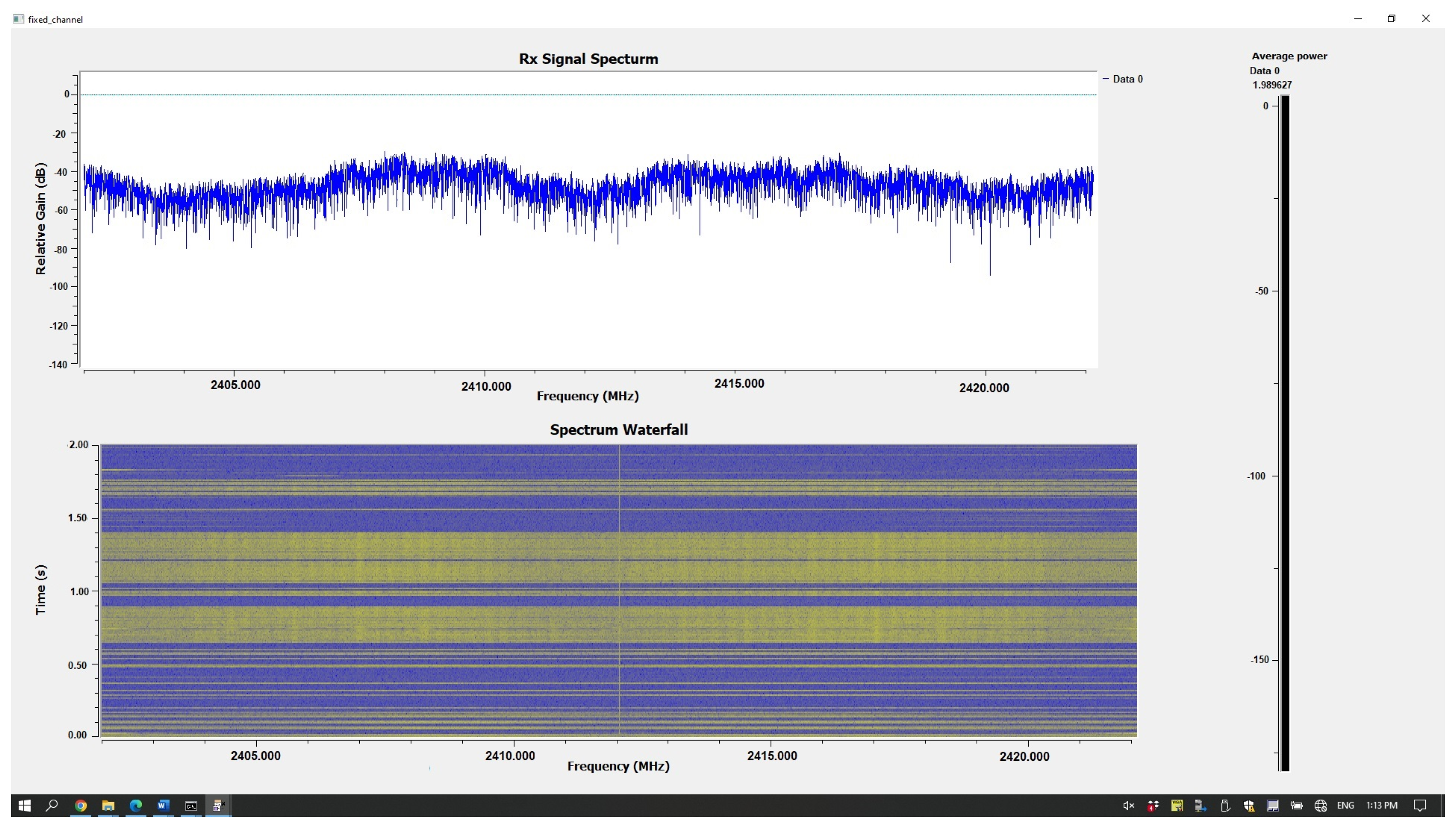
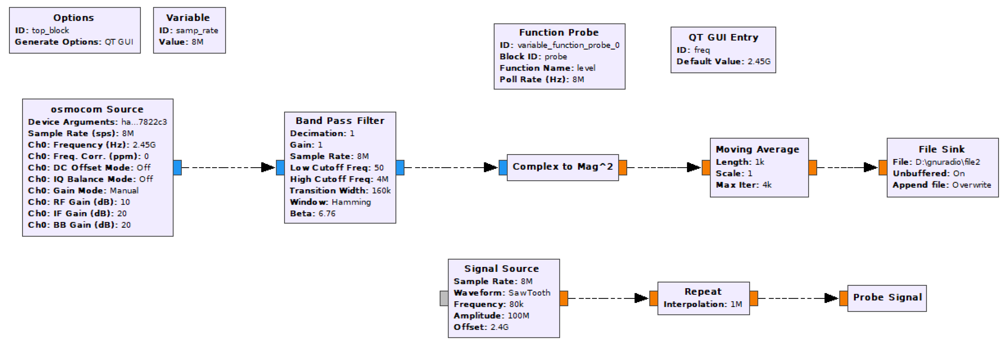
2.1.1. Fixed Channel Measurement

Given that this measurement pertains to a fixed channel configuration, supplementary data concerning the highest available Wi-Fi channel are supplied through the utilization of inSSIDer software 3.1.2.1, an open-source application. Figure 2 illustrates the standard dataset provided by inSSIDer, encompassing details such as the names of all accessible Wi-Fi networks, their respective Wi-Fi channel allocations, and the Received Signal Strength Indicator (RSSI). In this specific instance, one of the networks, labeled as “default”, employs the IEEE 802.11 b/g protocol and operates on Wi-Fi Channel 1, exhibiting a signal strength of −15 dBm. Within the scope of our system, the critical information furnished by inSSIDer pertains exclusively to the Wi-Fi channel. Each channel within the 2.4 GHz network operates within a bandwidth of 20 MHz, which corresponds to the maximum bandwidth that the HackRF receiver can accommodate. Having this information at hand, we can select the appropriate central frequency for the receiver.

Next, the implementation of the SDR-based RF measurement sub-system through GNU Radio is performed by means of a flowgraph comprising source (input) blocks, signal processing blocks, and output blocks. In the GRC environment, users construct a processing sequence by assembling these functional blocks, collectively referred to as a flowgraph.

Notably, each block can be easily customized through parameters specific to its functionality. The GNU Radio implementation of the initial version of the RF measurement sub-system, which is depicted in Figure 3, consists of the source block—osmocom (or Soapy HackRF)—and several other processing and illustration blocks for the graphical user interface (GUI).

The design parameters are set in the source block by means of two variables: central_freq—central frequency of the monitored Wi-Fi channel—and instantaneous bandwidth—which actually coincides with the sample rate (samp_rate).

The signal thus received is represented in frequency by means of two blocks: QT GUI Frequency Sink, which displays the spectrum of the received signal, and QT GUI Waterfall Sink, which illustrates the variation over time of the spectrum.

The original signal undergoes a multi-stage processing procedure. Initially, it is subject to filtration using a band-pass filter block characterized by the following parameters:

• Upper and lower cut-off frequencies, defined so that the DC component is rejected; therefore, f_{cutoff_1} = 50 Hz and f_{cutoff_2} = sample_rate/2;
• The use of a rectangular window, ensuring uniform attenuation of all frequencies beyond the region of interest, without introducing additional attenuation to frequencies close to the cut-off frequency;
• Employing a narrow transition width of 10 kHz, in order to facilitate rapid transitions between the passband zone and the rejection zone.

Then, the resulting signal, represented in complex format, undergoes processing to derive the spectral power density through the following steps:

• The complex signal is subjected to conjugation;
• The two sequences of values (the complex one and the conjugated one) are then multiplied, resulting in a real sequence of values that correspond to the magnitudes of the complex numbers, signifying the power density level;
• The average power within the designated frequency band is calculated by feeding the real signal into a sliding averaging block (MovingAverage), having as output the sum of the last N = 50000 samples, and divided by N;
• Subsequently, the computed average power is transformed into a logarithmic scale, resulting in a value expressed in decibels (dB). The Log10 block performs the following operation: output = n * log10 (input) + k, with the scalar multiplicative constant n = 10, and the scalar additive constant k being set to 0.

The outcome of this process is visually represented through the QT GUI Number Sink block and concurrently stored in a database. This database connection is established via the TCP Sink block.

The graphical interface resulting from running the configuration depicted above is illustrated in Figure 4. The graphical interface comprises the following elements: the upper section of the display reflects the outcome of the QT GUI Frequency Sink block, depicting the spectrum captured at the display moment. In the lower segment, a portrayal of the temporal progression of the measured spectrum is conveyed through a waterfall graphic, facilitated by the QT GUI Waterfall Sink block. Positioned on the right, the output showcased by the QT GUI Number Sink block signifies the average power within the measured channel.

2.1.2. Frequency Sweep Measurement

The second implementation, shown in Figure 5, represents a wideband power measurement system. The operating frequency of the HackRF receiver is modified in real time by probing a sawtooth signal and assigning that value to the carrier frequency using the set_freq function within the Python source code generated from the GNU Radio design. Thus, the operating frequency varies linearly within the 2.4 GHz 801.11 b Wi-Fi band, with a 1 MHz step. This yields a 100 MHz band, from 2.401 GHz to 2.5 GHz. The implementation can be generalized so that the HackRF device functions similarly to a spectrum analyzer in any frequency band within the HackRF 6 GHz operating band.

The Repeat/Interpolation block is used in order to perform multiple power measurements at the same operating frequency, before increasing the frequency value. Based on the chosen sample rate and interpolation factor, the device measures the received power without changing frequency, for a duration of 125 ms. A moving average with a size much smaller than the interpolation factor is used to smooth out the power measurements. These values are finally sent to a binary file, using 16-bit words for each sample. The binary file can be stored on a hard drive, flash drive or a Secure Digital Card (SD/microSD card), for further analysis.

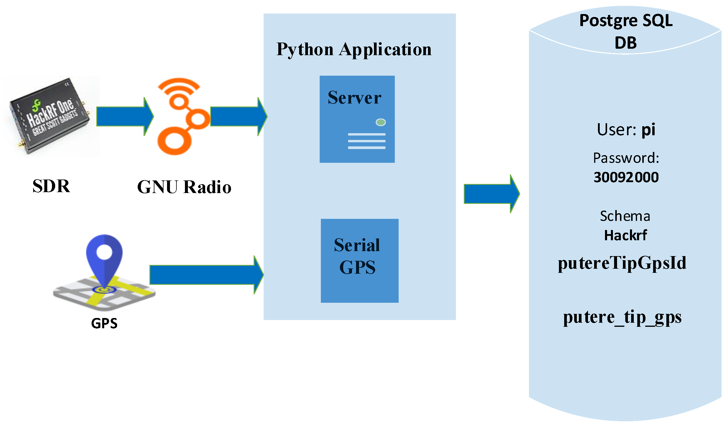
2.2. Measurement Data Processing Design

The measurement data include not only the RF average power, in dBs, furnished by the TCP (Transmission Control Protocol) Sink block, but also measurement date and time and user position information supplied by the GPS. The Adafruit Ultimate GPS HAT module provides GPS data in the NMEA (National Marine Electronics Association, Severna Park, MD, USA) format. It is designed to be compatible with the Raspberry Pi 400 device, and a physical connection between the GPS module and the Raspberry Pi 400 was established through the GPIO (General-Purpose Input/Output) port.

The spectral data processed via GNU Radio software and the georeferencing data are transmitted to a PostgreSQL database using a Python application. This Python application establishes a connection with the database using the credentials username and password. The data are then stored in the “power_type_gps” table within the “hackrf” section of the database.

To facilitate the integration between the GNU Radio interface, the GPS module, and the “hackrf” database, an application named “ServerPutereTipGps” was developed using the Python programming language. This application encompasses the following components:

• A server that receives data from GNU Radio;
• A connection to the serial port for receiving data from the GPS module;
• A connection to the “hackrf” database where information pertaining to power, frequency, and the system’s geographical coordinates are recorded.

A schematic representation outlining the fundamental principles of the Python application utilized for collecting the pertinent data is presented in Figure 6 and explained in the following paragraphs.

In the initial phase, the application establishes a connection with the ttyS0 serial port. This connection is realized through the instantiation of an object belonging to the serial class, which is part of the serial module. The messages emanating from the GPS module, affixed to the Raspberry Pi, are subsequently received and processed through this serial port interface. The configuration of this connection encompasses critical parameters, including the specification of a baud rate set at 9600, activation of parity, determination of the number of stop bits, and the setting of an output time value for data retrieval, expressed in seconds.

The GNU Radio program connects to the server through the TCP Sink block to send spectral information data, namely power ratings, which are recorded while running the GNU Radio flowgraph.

Then, the application makes a connection to the database, entering the name of the database, the user’s name, and the password to access it.

Subsequently, in the ensuing step, a TCP server is created, designed to listen on port 65434. The selection of this particular port number, which is notably a large integer, was made randomly to ensure its unavailability for other uses. Notably, the server and client functionalities are hosted on the same computing system, necessitating the utilization of the local address “127.0.0.1.”

The creation of a connection between the client and the server is achieved through the implementation of the socket class. This connection is instrumental in facilitating the bi-directional exchange of data in the form of bytes.

The command “conn, addr = s.accept()” is employed to instruct the application to await the establishment of a connection by GNU Radio on port 65434. This command, upon execution, not only identifies the address from which the connection originates but also generates a connection-type object. This object, in turn, enables the application to efficiently read and process the data transmitted by the client.

Upon establishing a connection with the TCP Sink, the Python application enters an infinite loop, wherein it continually reads the transmitted power values from GNU Radio using the command “data = conn.recv(4)”. Subsequently, these power values are stored in the database, alongside data originating from the GPS.

During the execution of the GNU Radio flowgraph, nominal power values are typically forwarded to the application. The GPS module has the capacity to record various details regarding the system’s geographical position, contingent upon the receipt of signals from an adequate number of satellites. Consequently, the code handles two distinct scenarios:

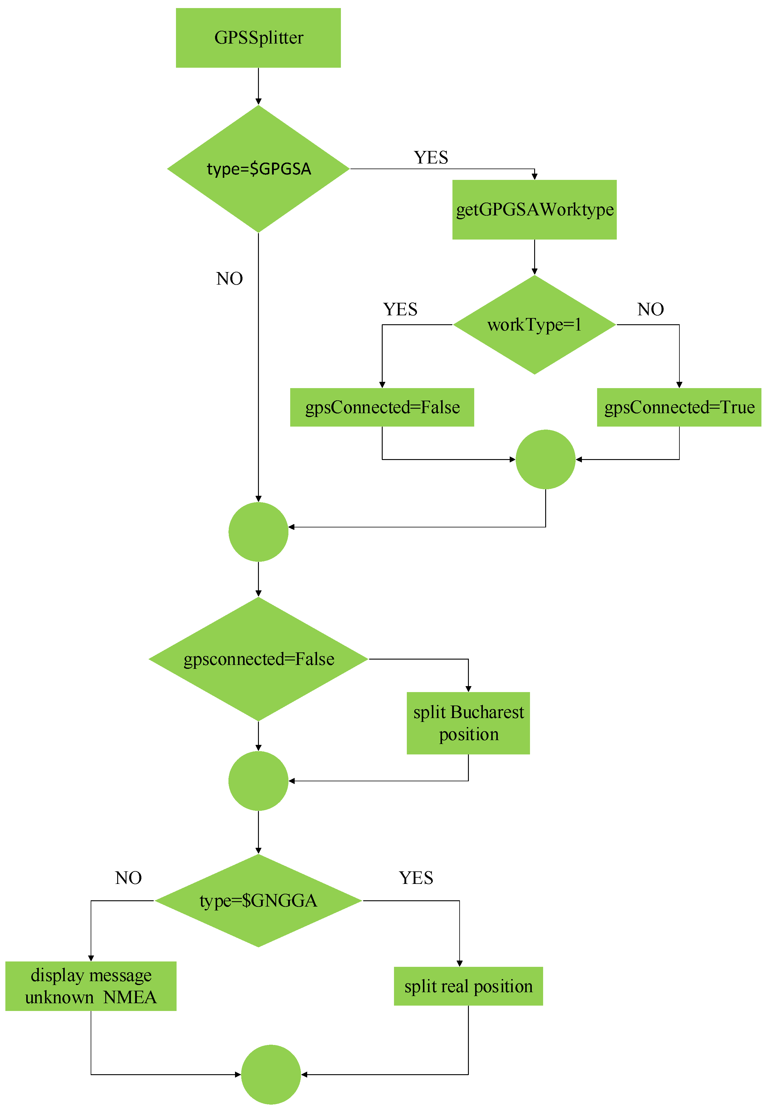
• If the GPS module does not receive any position-related data, identified by a message of type $GNGGA, the application proceeds to insert the position data for the city of Bucharest (44 degrees, 43 min north latitude; 26 degrees, 9 min east longitude) into the database. Simultaneously, it includes the nominal signal strength values received by the HackRF receiver;
• Conversely, if the GPS module successfully establishes a connection with the satellites, enabling it to determine the system’s precise position, the application records the actual positional data at the moment of program execution using the “insertPower(mydb, power [0], latitude, longitude, type)” command. Here, the “type” variable holds real-value data.

This iterative process continues indefinitely for as long as GNU Radio executes the flowgraph. If the client (GNU Radio) is halted, this infinite loop terminates. As a final step before shutting down the server, the database connection is closed using “mydb.close()”.

The GPS unit communicates with the application via the serial port, transmitting messages conforming to the NMEA standard. These messages are identified by codes commencing with a “$“ symbol. In this work, only two specific message types, namely GPGSA and GNGGA, were utilized. All pertinent values within each message type are extracted programmatically using the GPSSplitter class, which parses the messages based on comma separators. The resulting values are then stored within the respective class corresponding to the message type. To ascertain the specific data type received from the GPS module, the logical processes depicted in Figure 7 are adhered to.

If the received message type is $GPGSA, the third field, denoted as “workType,” plays a crucial role in ascertaining whether the GPS unit has established sufficient connections with satellites to initiate the position determination process. In accordance with the NMEA description of the GPGSA message, a value of 1 in this third field signifies that the requisite connections essential for determining the system’s position have not yet been established.

Following the reception of data from GNU Radio, the ServerPutereTipGps application proceeds to transmit all the essential data to the “power_gps_type” table within the database using the following SQL statement:

INSERT INTO power_gps_type (id, power, latitude, longitude, type, time)

VALUES (nextval(‘powerTipGpsId’), “+str(power)+”, ‘“+latitude+”’, ‘“+longitude+”’, ‘“+type+”’, NOW())”

This SQL statement leverages the sequence “power_type_gps_id” in conjunction with the “nextval” function, which serves to increment the value of the sequence utilized as the primary key in the database.

The function responsible for the insertion of data into the database takes several parameters, including the database connection, the nominal power values received from GNU Radio, the latitude and longitude coordinates of the location, the type of values characterizing the location, and the precise date and time at which the measurements were conducted.

In consideration of the variable signal reception capabilities of the GPS unit, which may or may not establish contact with a sufficient number of satellites to determine its position, the database records either real data when the GPS is connected or placeholder values when the GPS unit fails to calculate its position.

Within this function, a cursor, designated as “myCursor = mydb.cursor()”, is instantiated using the database connection. This cursor facilitates the execution of the SQL statement via the “myCursor.execute(sql)“ command. Subsequent to an INSERT SQL statement, the “mydb.commit()” command is invoked to finalize the data writing process.

In order to prevent the accumulation of unused open resources, especially given the constraints of the Raspberry Pi, which possesses limited memory, it is imperative to close the cursor using the “myCursor.close()” command.

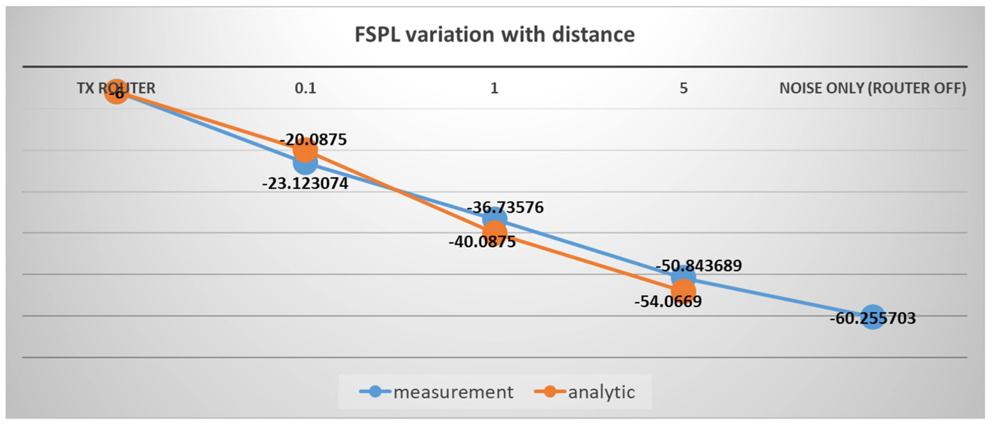
3. System Testing Results

The evaluation of the system involves a two-step process: first, a comparative examination of the performance of two distinct RF-EMF measurement unit versions is conducted; subsequently, an assessment of the operational efficacy of the portable measurement system is undertaken.

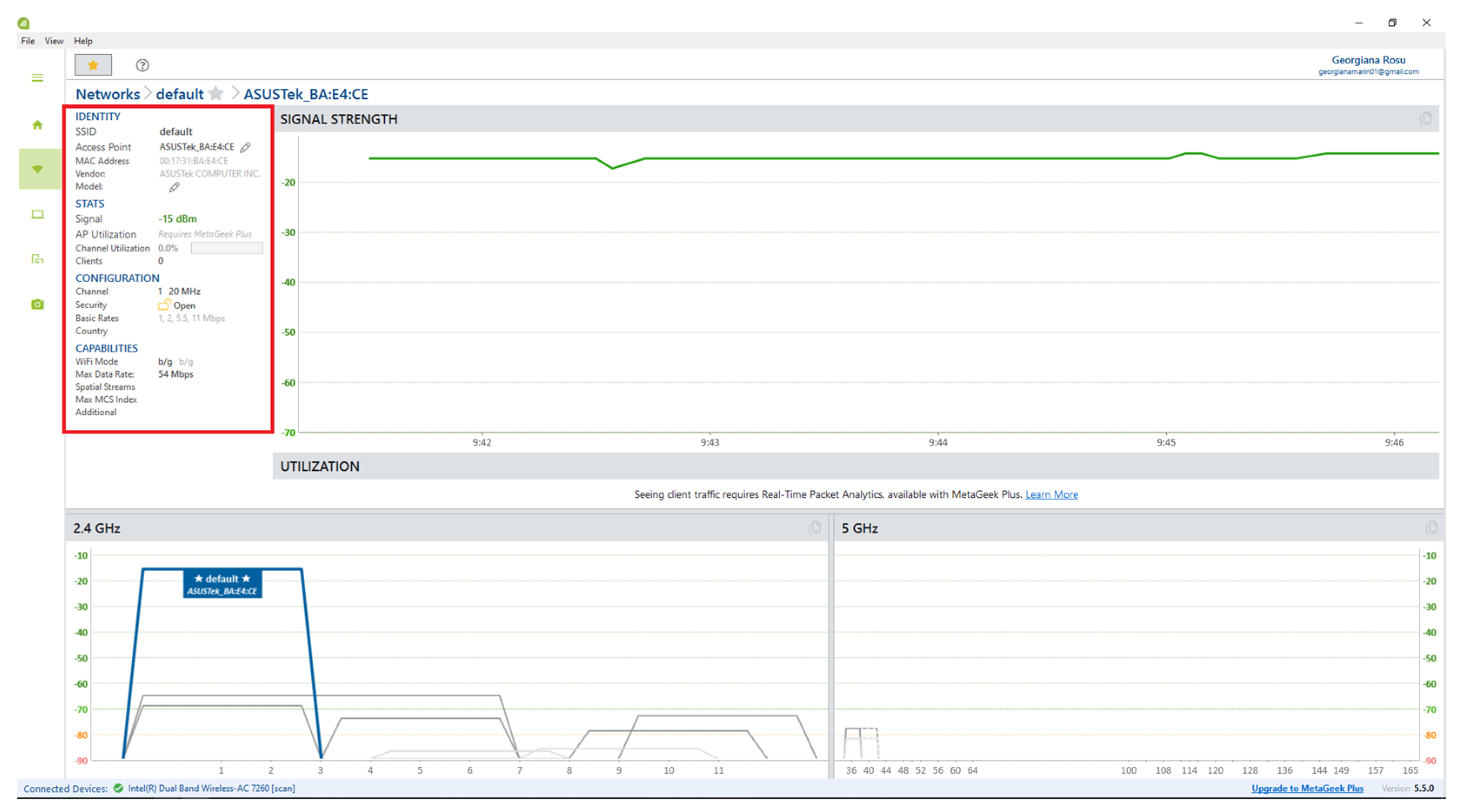
3.1. Comparative Testing of Two RF-EMF Measurement Unit Versions

In the first stage, the two versions of the RF unit implemented in GNU Radio were tested, with a specific focus on their capacity to deliver information compared to that obtained from a spectrum analyzer. The testing setup is illustrated in Figure 8 and consists of the following equipment:

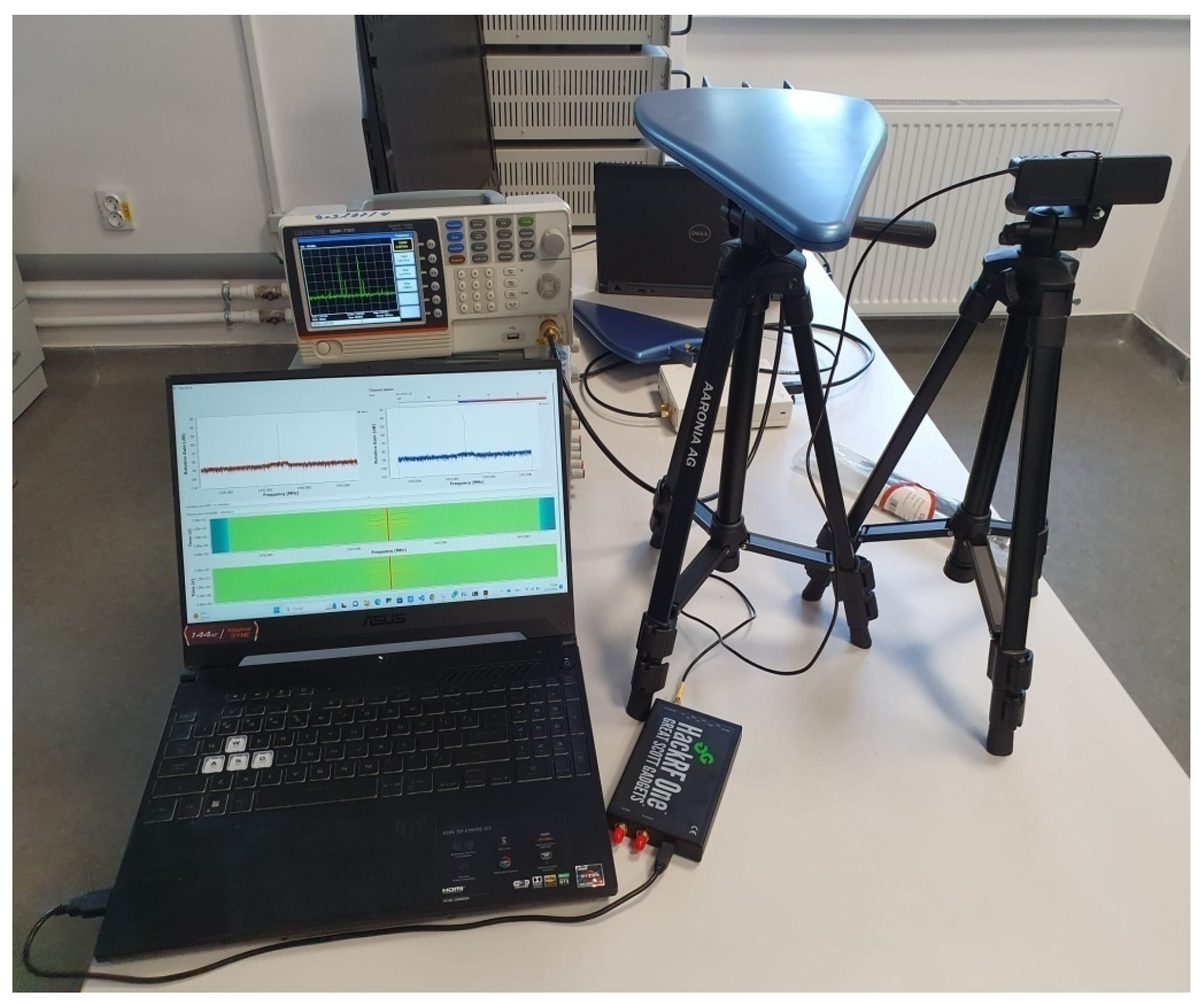
• A Wi-Fi router with a transmitting whip antenna (Tx), connected to the Internet through an Ethernet cable;
• The two configurations of the RF measurement unit, each consisting of a receiving (Rx) patch antenna and a HackRF device connected to a laptop; the HackRF device has an operating frequency ranging from 1 MHz to 6 GHz, with a bandwidth of 20 MHz, and the laptop runs with a 2.8 GHz Intel Core i7 CPU;
• A reference measurement device represented by a spectrum analyzer (SA)—Aaronia Spectran 6080-V4, which operates in the 10 MHz–8 GHz band, and a receiving log-periodic directional antenna Aaronia HyperLog 7025, with a 5 dB gain. The spectrum analyzer is connected to a laptop with dedicated software (Aaronia MCS Spectrum Analyzer Software 2.1.6.

As noted in the diagram illustrated in Figure 8 and the image in Figure 9, the generator unit and the Rx antennae are placed on the left-side table, whereas on the right-side table, there are the RF receivers, the spectrum analyzer, and two laptops.

The log-periodic antenna was placed between the two Rx antennae, so that the distance between two adjacent antennae was approximately 20 cm. The distance between the Tx antenna and the receiving antennae was approximately 70 cm, thus placing the receiving antennae in the far-field region. The spectrum analyzer (SA) was connected to the same laptop as the initial RF unit configuration—the one connected to the Rx 1 antenna.

In the experimental configuration, one of the two laptops established an Internet connection through the access point facilitated by the router and accessed web pages characterized by high data content, particularly involving video streaming. This deliberate choice aimed to augment the emitted power from the generator in a manner analogous to authentic ambient exposure scenarios.

The outcome, as provided by the QT GUI Frequency Sink block (in Figure 3), delineated the Wi-Fi signal spectrum within the band corresponding to the operational channel. These outcomes were subsequently juxtaposed with the signal spectrum acquired through the SA. Figure 10 serves to illustrate a comparative analysis of the spectra obtained from these two devices—the SA, positioned at the lower section of the image, and the SDR device configured in its initial state, specifically the fixed channel configuration.

In order to test the performance of the second version of the SDR implementation—the frequency sweep configuration presented in Section 2.1.2—a number of measurements were also performed simultaneously with the ones already mentioned. The Wi-Fi router was configured for 802.11 b and used as a transmitter, for video traffic, in two distinct scenarios: Wi-Fi auto-channel selection and single channel (channel 6). The video transmission and Wi-Fi power measurement lasts around a minute. This way, the entire 2.4 GHz band can be swept multiple times and a spectrogram can be formed. The power measurements for the Wi-Fi auto-channel transmission were analyzed in MATLAB and are presented in spectrogram form in Figure 11.

The non-scaled spectrogram in Figure 11a shows that the transmission is carried out within multiple channels of the 2.4 GHz band, while the scaled version (Figure 11b) shows that there is no significant power discrepancy between the signals received on different frequencies. Similar results are presented in Figure 12. Both average and close-to-maximum-power histograms show that a wideband transmission was performed.

The second scenario had the Wi-Fi router prioritizing channel 6 for the video transmission. Indeed, in this case, both the spectrogram and histogram presented in Figure 13 show that most of the Wi-Fi signal power was received for frequencies within channel 6 (2426–2448 MHz). The spectrogram highlights the 2430–2440 MHz band.

3.2. Portable System Testing

The second testing phase studied the performance of the overall measurement system, combining the RF-EMF measurement unit, the GPS georeferencing unit, and the data processing and storage component implemented through the Raspberry Pi.

The initial version of the system integrates the RF-EMF unit in a fixed channel configuration. This choice is justified by its inherent simplicity and by the fact that it provides a single piece of data to be fed into the database—the average channel power.

The measurements were performed in a controlled environment, a shielded chamber, under normal conditions. Otherwise, the test signal could be influenced by fading or by interferences with unwanted radio sources, which could significantly fluctuate the received power. The experiment could have also been influenced by other factors such as temperature or even the housing environment (wall material/thickness) in which the power measurement took place [23,24,25,26].

The system underwent testing against the parameters outlined by a spectrum analyzer, and both devices were placed outside of the shielded chamber, as shown in Figure 14. This evaluation was conducted within a scenario involving the access of a web page designed to assess connection quality, thereby engaging both the upload and download bandwidths of the channel.

Subsequently, the system’s performance was assessed in terms of the variation in the average power within the channel at different distances from the source. Three specific distances, namely 0.1 m, 1 m, and 5 m, were employed for this analysis. The measurements were compared to the analytical results provided by the free-space path loss (FSPL) parameter, computed with the following relation [23]:

$$FSPL=20 {\log }_{10}\left(d\right)+20 {\log }_{10}f+20 {\log }_{10}\left(\frac{4\pi }{c}\right)-G_t-G_r$$

(1)

Here, d represents the distance to the source, f—the frequency, c—the free-space speed of light, and G_t and G_r indicate antenna Tx and Rx antenna gains, respectively, and are both considered to be 3 dBi. In this instance, the frequency f = 2412 MHz was chosen, and distance was successively given the three values indicated above.

The comparative analysis of the FSPL parameter is illustrated in Figure 15, with the analytical results obtained from Equation (1) illustrated with orange dots, while the experimental ones are noted with blue dots.

The ultimate outcome delivered by the portable system manifests as a database (DB). Figure 16 outlines a schematic depiction of the dataflow and provides the access credentials for the PostgreSQL DB.

In Figure 17, a segment of the database content is presented. Within this illustration, the “id” field serves as the primary database key, the “putere” (power) field signifies the channel’s average power as measured by the RF unit, and the subsequent “latitudine” and “longitudine” fields denote the geographical coordinates furnished by the GPS unit. Additionally, the “tip” field distinguishes whether the location was directly measured or replaced with a default value (representing the central geographical position of Bucharest) in instances of poor GPS reception, primarily attributed to adverse weather conditions. Lastly, the “timp” field corresponds to the timestamp associated with the measurements.

4. Discussion

The initial testing aimed to determine the efficiency of the SDR system in a fixed channel configuration against the indications of a SA operating in the same frequency band—corresponding to a particular Wi-Fi channel. Both devices were operated under two distinct scenarios:

• The receiver was linked to the router without soliciting data from the Internet network;
• The receiver, via the router, accessed web pages featuring substantial data content.

In both instances, a noteworthy correlation was discerned between the graphical depiction generated by the QT GUI Frequency Sink block and the spectrum analyzer’s representation.

The second SDR configuration was designed as an optimized version of the former, in terms of frequency band and data content. The frequency sweep SDR configuration broadens the operating frequency band, allowing power measurements to be performed for wideband EMF sources. The HackRF-based implementation is highly configurable, mobile, and has a smaller size and lower cost compared to conventional spectrum analyzers.

The proposed design can be customized with regard to operating frequency band, sample time, measurement time for each frequency bin, data averaging, sample size, and the option to store the measured power samples as nominal values or in dBm. The measured data are stored in a binary file or database. The size of this file can be reduced by lowering either the sample time or the sample size, which is 16-bit by default, for each measured power value. The configuration was successfully tested in a shielded chamber using a 2.4 GHz Wi-Fi transmitter. The system’s functionality was verified by analyzing the measured power data in MATLAB for two scenarios: multi-channel and single-channel video transmissions.

Using the frequency sweep configuration, the system can monitor and perform power measurements for a maximum spectrum of 6 GHz, constrained by the SDR operating frequency band. Increasing the measurement band would normally result in a longer sweep time, which could cause certain short-duration components to not be registered by the system. The sweep time is given by the period of a sawtooth or staircase signal assigned to the operating frequency of the SDR device. This period can be reduced in order to perform a faster sweep and minimize the loss of any short-term fluctuations that may occur. The drawback would be that, for a fixed sample rate, the number of samples within the sawtooth period would decrease, which means that the spectrum will have a reduced number of points or that the frequency step increases. This compromise between sweep time and frequency step size, which are inversely proportional, can be solved within GNU Radio with a parameter that adjusts, if possible, the sample rate for the sawtooth signal, according to the desired measurement band size. As presented in Section 2.1.2, the system also has the option to perform and average multiple power measurements at the same frequency before moving to the next, so reducing the time spent at each frequency constitutes a solution for an improved wideband functionality, with regard to detecting short-term fluctuations.

Nevertheless, the choice of the initial configuration was motivated by its inherent simplicity and its subsequent implementation on the portable system. Subsequent testing involved the execution of the frequency band corresponding to a designated Wi-Fi channel, with channel 6 being the initial selection. The sweep time was set at approximately 100 milliseconds for each iteration. In each run, a singular data element, specifically the average power of the channel, was recorded and added to the database.

The results of the portable system with the implementation of the initial configuration can be used to create an electromagnetic field profile map depending on the geographical coordinates. A typical result illustrating the average measured power is depicted in Figure 18. The data were obtained using the initial configuration of the RF unit, with in situ measurements in a single Wi-Fi channel with bandwidth 20 MHz. The level is color-coded, with the scale represented on the right side of the map.

Regarding the system’s use in a practical scenario, there are some issues that need to be considered. First, the power measurement may be influenced by fading or by interferences with unwanted radio signals. A solution to this could be spatial diversity, that is, using multiple antennas or an antenna array to receive the radio signal and use specific techniques like beamforming to separate each signal source and measure their power independently. Another issue would regard the system’s portability and power supply. Fortunately, both HackRF and Raspberry Pi devices can be powered via USB (3.3 V and 5 V, respectively) which means that any external batteries or power banks with USB interfaces can be used. Regarding the system’s geolocation capability, the signal strength can be affected by a number of factors like atmospheric conditions or signal-blocking devices and obstacles. Solutions here could be to employ frequency and spatial diversity, by using a multi-frequency and multi-constellation receiver, like the GNSS (Global Navigation Satellite System), that can be software-defined.

The system can be further improved by migrating the concept to a RFSoC (Radio Frequency System on Chip) implementation, which integrates high-speed ADCs/DACs, real-time and application processing units, high storage capacity, and programmable logic for high-speed processing. This architecture would incorporate the SDR and Raspberry Pi functionality and would enable power measurements to be performed in real time without needing to demodulate the received signal. The main drawback of this solution would be its increased cost.

The proposed solution primarily functions as an EMF spectrum monitoring system with the capability to measure the average field value. Using SDR modeling and Python programming, we designed a portable system, programmed with custom in-house software, that could function as a reduced-size system combining the capabilities of a spectrum analyzer and an exposimeter. While setting up the experimental tests, we based our procedures on the assumption that the system would not be directly attached to the user’s body. The system could, however, be placed in a hand-held container, which could be carried by the user while moving and placed in close vicinity while the user is stationary. This way, the practical measurements could correlate with the tests performed and presented in this paper.

5. Conclusions

This paper proposes an SDR-based system to perform an accurate and exhaustive measurement of RF-EMF exposure in urban areas. The uniqueness of the proposed system arises from its advanced features compared to limited-performance exposimeters in the commercial market, which mainly use narrow-band sensors. This enhancement is accomplished by utilizing Software-Defined Radio (SDR) technology to widen the frequency bandwidth and enable the detection of short-term fluctuations in signal spectra.

Exposimeters currently available on the market, even those considered highly efficient, such as those with measurement georeferencing capabilities, operate on the fundamental principle of averaging measurement results over a specified time interval. This principle was investigated and implemented in the initial configuration under scrutiny. The initial iteration, subjected to laboratory and in situ testing, yields data comparable to a Commercial Off-The-Shelf (COTS) exposimeter. In our research methodology, we did not only assess overall exposure but also endeavored to detect short-term fluctuations in RF-EMF levels.

The optimized version, utilizing a frequency sweep configuration, facilitates the acquisition and processing of field data that surpasses the capabilities of commercially available devices, particularly in terms of spectral content. The testing included multiple scenarios associated with channels and frequency bands. The acquired outcomes were compared with the readings from a spectrum analyzer, effectively capturing temporal variations in the spectrum of the measured signal.

Notably, this optimized version does not confine itself to displaying exposure doses for predefined time intervals. Instead, it enables the storage of spectral component levels across a bandwidth exceeding the instantaneous capacity of the SDR system. This is achieved through the spectrum sweeping solution implemented in GNU Radio, as illustrated in Figure 5. We highlighted the fact that this configuration underwent laboratory testing exclusively, as detailed in Section 4. Furthermore, the Discussion section underscores that the acquired data are transformed into binary code and stored. It is essential to acknowledge that this configuration necessitates expanding the database to accommodate the substantial volume of data recorded for each sweep. This stands in contrast to conventional approaches that rely on a singular value representing the average power in a channel over a specified timeframe.

Further testing will encompass extensive in situ measurements and comparisons with the indications of a high-end exposimeter and a spectrum analyzer. Subsequent investigations will be focused on the deployment of the optimized SDR configuration—the frequency sweep configuration—and the adjustment of the database, with particular attention paid to aligning the compatibility of the two software components within the system, while also considering the available computing resources.

References

1. Chou, C.-K. Controversy in Electromagnetic Safety. Int. J. Environ. Res. Public Health 2022, 19, 16942. [Google Scholar] [CrossRef]
2. Bartosova, K.; Neruda, M.; Vojtech, L. Methodology of Studying Effects of Mobile Phone Radiation on Organisms: Technical Aspects. Int. J. Environ. Res. Public Health 2021, 18, 12642. [Google Scholar] [CrossRef]
3. Sârbu, A.; Miclău, S.; Digulescu, A.; Bechet, P. Comparative Analysis of User Exposure to the Electromagnetic Radiation Emitted by the Fourth and Fifth Generations of Wi-Fi Communication Devices. Int. J. Environ. Res. Public Health 2020, 17, 8837. [Google Scholar] [CrossRef]
4. Redmayne, M.; Maisch, D. ICNIRP Guidelines’ Exposure Assessment Method for 5G Millimetre Wave Radiation May Trigger Adverse Effects. Int. J. Environ. Res. Public Health 2023, 20, 5267. [Google Scholar] [CrossRef]
5. Vijayalaxmi. Biological and health effects of radiofrequency fields: Good study design and quality publications. Mutat. Res. Genet. Toxicol. Environ. Mutagen. 2016, 810, 6–12. [Google Scholar] [CrossRef]
6. Panagopoulos, D.J.; Johansson, O.; Carlo, G.L. Real versus Simulated Mobile Phone Exposures in Experimental Studies. BioMed Res. Int. 2015, 2015, 607053. [Google Scholar] [CrossRef]
7. Tsatsakis, A.M.; Kouretas, D.; Tzatzarakis, M.N.; Stivaktakis, P.; Tsarouhas, K.; Golokhvast, K.S.; Rakitskii, V.N.; Tutelyan, V.A.; Hernandez, A.F.; Rezaee, R.; et al. Simulating real-life exposures to uncover possible risks to human health: A proposed consensus for a novel methodological approach. Hum. Exp. Toxicol. 2017, 36, 554–564. [Google Scholar] [CrossRef] [PubMed]
8. Tognola, G.; Plets, D.; Chiaramello, E.; Gallucci, S.; Bonato, M.; Fiocchi, S.; Parazzini, M.; Martens, L.; Joseph, W.; Ravazzani, P. Use of Machine Learning for the Estimation of Down- and Up-Link Field Exposure in Multi-Source Indoor WiFi Scenarios. Bioelectromagnetics 2021, 42, 550–561. [Google Scholar] [CrossRef] [PubMed]
9. Spandole-Dinu, S.; Catrina, A.-M.; Voinea, O.; Andone, A.; Radu, S.; Haidoiu, C.; Călborean, O.; Popescu, D.; Suhăianu, V.; Baltag, O.; et al. Pilot Study of the Long-Term Effects of Radiofrequency Electromagnetic Radiation Exposure on the Mouse Brain. Int. J. Environ. Res. Public Health 2023, 20, 3025. [Google Scholar] [CrossRef] [PubMed]
10. Kostoff, R.N.; Heroux, P.; Aschner, M.; Tsatsakis, A. Adverse health effects of 5G mobile networking technology under real-life conditions. Toxicol. Lett. 2020, 323, 35–40. [Google Scholar] [CrossRef] [PubMed]
11. Urbinello, D.; Joseph, W.; Verloock, L.; Martens, L.; Röösli, M. Temporal trends of radio-frequency electromagnetic field (RF-EMF) exposure in everyday environments across European cities. Environ. Res. 2014, 134, 134–142. [Google Scholar] [CrossRef] [PubMed]
12. Atanasova, G.; Atanasov, B.; Atanasov, N. Assessment of Electromagnetic Field Exposure on European Roads: A Comprehensive In Situ Measurement Campaign. Sensors 2023, 23, 6050. [Google Scholar] [CrossRef]
13. Mallik, M.; Tesfay, A.; Allaert, B.; Kassi, R.; Egea-Lopez, E.; Molina-Garcia-Pardo, J.-M.; Wiart, J.; Gaillot, D.; Clavier, L. Towards Outdoor Electromagnetic Field Exposure Mapping Generation Using Conditional GANs. Sensors 2022, 22, 9643. [Google Scholar] [CrossRef] [PubMed]
14. Petroulakis, N.; Mattsson, M.-O.; Chatziadam, P.; Simko, M.; Gavrielides, A.; Yiorkas, A.; Zeni, O.; Scarfi, M.; Soudah, E.; Otin, R.; et al. NextGEM: Next-Generation Integrated Sensing and Analytical System for Monitoring and Assessing Radiofrequency Electromagnetic Field Exposure and Health. Int. J. Environ. Res. Public Health 2023, 20, 6085. [Google Scholar] [CrossRef] [PubMed]
15. Onishi, T.; Esaki, K.; Tobita, K.; Ikuyo, M.; Taki, M.; Watanabe, S. Large-Area Monitoring of Radiofrequency Electromagnetic Field Exposure Levels from Mobile Phone Base Stations and Broadcast Transmission Towers by Car-Mounted Measurements around Tokyo. Electronics 2023, 12, 1835. [Google Scholar] [CrossRef]
16. Mulugeta, B.; Wang, S.; Chikha, W.B.; Liu, J.; Roblin, C.; Wiart, J. Statistical Characterization and Modeling of Indoor RF-EMF Down-Link Exposure. Sensors 2023, 23, 3583. [Google Scholar] [CrossRef]
17. Bonato, M.; Dossi, L.; Chiaramello, E.; Fiocchi, S.; Tognola, G.; Parazzini, M. Stochastic Dosimetry Assessment of the Human RF-EMF Exposure to 3D Beamforming Antennas in indoor 5G Networks. Appl. Sci. 2021, 11, 1751. [Google Scholar] [CrossRef]
18. Deprez, K.; Colussi, L.; Korkmaz, E.; Aerts, S.; Land, D.; Littel, S.; Verloock, L.; Plets, D.; Joseph, W.; Bolte, J. Comparison of Low-Cost 5G Electromagnetic Field Sensors. Sensors 2023, 23, 3312. [Google Scholar] [CrossRef]
19. Van Torre, P.; Agneessens, S.; Aminzadeh, R.; Thielens, A.; Bossche MV, D.; Joseph, W.; Rogier, H. Wearable multi-antenna multi-band measurement system for personal radio-frequency exposure assessment. In Proceedings of the European Medical and Biological Engineering Conference, Singapore, 13 June 2017; pp. 687–690. [Google Scholar]
20. Urbinello, D.; Huss, A.; Beekhuizen, J.; Vermeulen, R. Use of portable exposure meters for comparing mobile phone base station radiation in different types of areas in the cities of Basel and Amsterdam. Sci. Total Environ. 2014, 468–469, 1028–1033. [Google Scholar] [CrossRef]
21. Aminzadeh, R.; Thielens, A.; Gaillot, D.P.; Lienard, M.; Kone, L.; Agneessens, S.; Van Torre, P.; Van den Bossche, M.; Verloock, L.; Dongus, S.; et al. A Multi-Band Body-Worn Distributed Exposure Meter for Personal Radio-Frequency Dosimetry in Diffuse Indoor Environments. IEEE Sens. J. 2019, 19, 6927–6937. [Google Scholar] [CrossRef]
22. Celaya-Echarri, M.; Azpilicueta, L.; Karpowicz, J.; Ramos, V.; Lopez-Iturri, P.; Falcone, F. From 2G to 5G Spatial Modeling of Personal RF-EMF Exposure Within Urban Public Trams. IEEE Access 2020, 8, 100930–100947. [Google Scholar] [CrossRef]
23. Machado-Fernández, J.R. Software Defined Radio: Basic Principles and Applications. Rev. Fac. De Ing. 2015, 24, 79–96. [Google Scholar] [CrossRef]
24. Wang, Y.; Wang, C.; Lian, P.; Xue, S.; Liu, J.; Gao, W.; Shi, Y.; Wang, Z.; Yu, K.; Peng, X.; et al. Effect of Temperature on Electromagnetic Performance of Active Phased Array Antenna. Electronics 2020, 9, 1211. [Google Scholar] [CrossRef]
25. Lee, H.; Ahn, C.; Choi, N.; Kim, T.; Lee, H. The Effects of Housing Environments on the Performance of Activity-Recognition Systems Using Wi-Fi Channel State Information: An Exploratory Study. Sensors 2019, 19, 983. [Google Scholar] [CrossRef] [PubMed]
26. Radhakrishna, K.S.; Lee, Y.S.; You, K.Y.; Thiruvarasu, K.M.; Ng, S.T. Study of Obstacles Effect on Mobile Network Study of Obstacles Effect on Mobile Network. INTL J. Electron. Telecommun. 2023, 69, 155–161. [Google Scholar] [CrossRef]
Figure 1. Diagram of the EMP exposure measurement system.
Electronics 12 05003 g001
Figure 2. WiFi network information provided by inSSIDer software.
Electronics 12 05003 g002
Figure 3. GNU Radio flowgraph of the fixed-channel average power measurement configuration.
Electronics 12 05003 g003
Figure 4. Graphical interface of the fixed channel measurement configuration.
Electronics 12 05003 g004
Figure 5. GNU Radio diagram of the frequency sweep measurement configuration.
Electronics 12 05003 g005
Figure 6. Flowchart of the Python application for the storage of measurement data in a database.
Electronics 12 05003 g006
Figure 7. Flowchart of the program establishing GPS coordinates.
Electronics 12 05003 g007
Figure 8. Schematic setup of the testing of the two RF unit configurations compared to a spectrum analyzer.
Electronics 12 05003 g008
Figure 9. Testing setup of the two RF unit configurations compared to a spectrum analyzer.
Electronics 12 05003 g009
Figure 10. Comparison of the indications of the fixed channel configuration—QT GUI Frequency Sink block (upper side) versus the spectrum analyzer (lower side).
Electronics 12 05003 g010
Figure 11. Spectrogram results for the full-band (auto-channel) Wi-Fi video transmission: (a) not scaled; (b) scaled with the absolute maximum value.
Electronics 12 05003 g011
Figure 12. Histograms for the Wi-Fi channel occurrences regarding the channel power: (a) higher than the average received power; (b) being at least 90% of the maximum received power.
Electronics 12 05003 g012
Figure 13. Power measurement results for single-channel Wi-Fi video transmission: (a) spectrogram scaled to the maximum value; (b) histograms for the Wi-Fi channel occurrences.
Electronics 12 05003 g013
Figure 14. Testing setup of the portable system against the spectrum analyzer.
Electronics 12 05003 g014
Figure 15. The free-space path loss (FSPL) variation with distance.
Electronics 12 05003 g015
Figure 16. Dataflow schematic diagram and database credentials.
Electronics 12 05003 g016
Figure 17. Excerpt of the database results.
Electronics 12 05003 g017
Figure 18. Typical representation of the database results on an electromagnetic field map.
Electronics 12 05003 g018
Disclaimer/Publisher’s Note: The statements, opinions and data contained in all publications are solely those of the individual author(s) and contributor(s) and not of MDPI and/or the editor(s). MDPI and/or the editor(s) disclaim responsibility for any injury to people or property resulting from any ideas, methods, instructions or products referred to in the content.