Harmonic State Estimation in Power Systems Using the Jaya Algorithm

Abstract

The increasing use of nonlinear loads in power systems introduces voltage and current components at non-fundamental frequencies, leading to harmonic distortion, which negatively impacts electrical and electronic devices. A common mitigation strategy involves identifying harmonic sources and installing filters nearby. However, due to the high cost of power quality (PQ) meters, comprehensive harmonic level monitoring across the entire power system is impractical. To address this, various methodologies for Harmonic State Estimation (HSE) have been developed, which estimate distortion levels on unmonitored system buses using data from a minimal set of monitored ones. Many HSE techniques rely on optimization algorithms with numerous tuning parameters, complicating their application. This paper proposes a novel methodology for fundamental frequency power flow and harmonic state estimation using the Jaya algorithm, which is characterized by fewer tuning parameters for easier adjustment. It also introduces a strategy to determine the minimal number of buses that need monitoring to achieve system observability. The methodology is validated on the IEEE-14 and IEEE-30 bus systems, demonstrating its effectiveness. The results of the proposed methodology are compared with those obtained using Evolutionary Strategies (ESs), highlighting its enhanced accuracy and computational efficiency.

1. Introduction

Over the decades, the increase in nonlinear loads, such as LED lighting systems, frequency inverters, and rectifiers, has introduced harmonic components into power systems. These components have significant negative effects on the operation of equipment supplied by waveforms distorted by harmonics [1].

The continuous evolution of power systems, along with the growing use of nonlinear loads, has highlighted the importance of harmonic distortion and its potential to affect system performance and reliability. This emphasizes the need to develop HSE methodologies to identify harmonic sources, allowing for their treatment and mitigation.

In 1970, initial efforts in the field of power system state estimation by [2,3,4] provided a fundamental framework to address these challenges, setting a benchmark for future research in HSE. The main advantage of this methodology lies in its ability to provide a comprehensive framework for system analysis, although its direct applicability to HSE was limited due to the lack of focus on harmonic distortions.

Subsequent advancements were made by [5] in 1989, who introduced a new state estimation technique specifically aimed at identifying harmonic sources, a crucial development in the field of HSE. However, the effectiveness of this approach was contingent upon the quality of the available measurement data.

In 1991, Beides and Heydt [6] expanded the scope of HSE by incorporating the Kalman filter for a dynamic estimation of harmonic states. This innovation allowed for adaptation to the dynamic variations of systems, although challenges related to computational complexity and the need for accurate modeling limited its applicability.

The exploration of the potential of neural networks by Hartana and Richards [7] in 1990 introduced an adaptive methodology for monitoring and identifying harmonic sources, noted for its flexibility. The main limitation, however, was the dependence on the quality of training data and the specific architecture of the neural network used.

Advancing HSE using the least squares method, a hybrid nonlinear method based on the least squares method and Kirchhoff’s current laws was introduced by [8]. One of the main disadvantages noted was that the accuracy of the estimate decreased with the harmonic order to be estimated.

In 1992, artificial neural networks were also used by [9] for the estimation of harmonic voltages. The results were compared with those obtained with known methods up to that time, yielding good results in terms of accuracy.

A methodology using the least squares method in conjunction with Singular Value Decomposition (SVD) was presented by Lobos et al. [10]. Despite satisfactory results, this technique requires greater computational effort and longer processing time than other techniques.

In 2004, the SVD technique was applied to the three-phase HSE of partially observable electrical systems [11]. Although the technique proved reliable and computationally stable, the SVD technique requires more time and processing cost than traditional techniques.

In 2005, a technique using neural networks for HSE from a reduced number of meters was proposed by [12]. In this technique, neural networks are initially used to provide pseudo-measurement values based on available measurements. These values are improved using state estimation with redundant measurements. The performance was satisfactory for the simulations carried out; however, obtaining good results is tied to the location of the meters.

Arruda et al. [13] advanced the use of ESs for harmonic distortion estimation, providing robustness and adaptability to the HSE process. However, this technique presents several parameters that need to be empirically adjusted. Thus, the selection and configuration of evolutionary parameters emerged as critical challenges for the effectiveness of this technique. A limitation of the presented methodology is that it only estimates the harmonic components of the network, assuming that the PQ meter data are synchronized and that the power flow for the entire electric power system (EPS) at the fundamental frequency is known.

Also in 2010, Arruda et al. [14] presented a study of HSE based on Evolutionary Strategies, however, performing a three-phase analysis of the power system. The results were compared with those obtained using the traditional Monte Carlo technique. The robustness of the proposed method was hindered by the adjustment of numerous HSE parameters for algorithm convergence, as well as the need for meter synchronization and prior knowledge of power flow in all EPS bars and phases.

Sepulchro, Encarnação, and Brunoro introduced an algorithm in 2014 [15] for estimating both harmonic distortion and power flow at the fundamental frequency, leveraging Evolutionary Strategies. This research extends the application of HSE by incorporating the estimation of fundamental power flow. However, it also encounters difficulties related to the fine-tuning of ES parameters.

In 2021, a hybrid algorithm for HSE in a transmission EPS from a reduced number of meters was proposed by [16]. A strategy called “HA” was used, which is a combination of ES algorithms with SADE. SADE is a type of modified Differential Evolution algorithm. The goal is to combine the high convergence speed of ES with the excellent accuracy of SADE. The technique was applied to the IEEE 14-bus and IEEE 57-bus systems, and the results obtained are satisfactory; however, the technique encountered a number of parameters involved in the combination of the two algorithms.

The introduction of the Jaya algorithm for solving multi-objective optimal power flow by Warid et al. in 2018 [17] brought a new perspective on the use of optimization algorithms with few parameters in various problems. This work highlighted the efficiency and simplicity of the Jaya algorithm as valuable features to tackle optimization problems in power systems, such as HSE. The simplicity of the code, underscored by its few tuning parameters, makes the Jaya algorithm a promising tool for HSE, particularly in larger electrical systems where complexity renders established methods like Evolutionary Strategies impractical.

In 2024, a technique for optimal power flow analysis to minimize power losses was proposed by [18]. This technique is based on two optimization methods, the Jaya algorithm, and the Teacher Learning Based Optimization (TLBO) algorithm. The absence of parameters in both algorithms makes the proposed technique less complex. The technique was applied to the IEEE 39-bus system. Also in 2024, Sepulchro and Encarnação extended the application of the Jaya algorithm to HSE [19]. In this paper, preliminary results using the Jaya algorithm were presented for harmonic state and power flow estimation for the IEEE 14-bus system. The main objective of this work was just to validate the Jaya algorithm on a small-scale system.

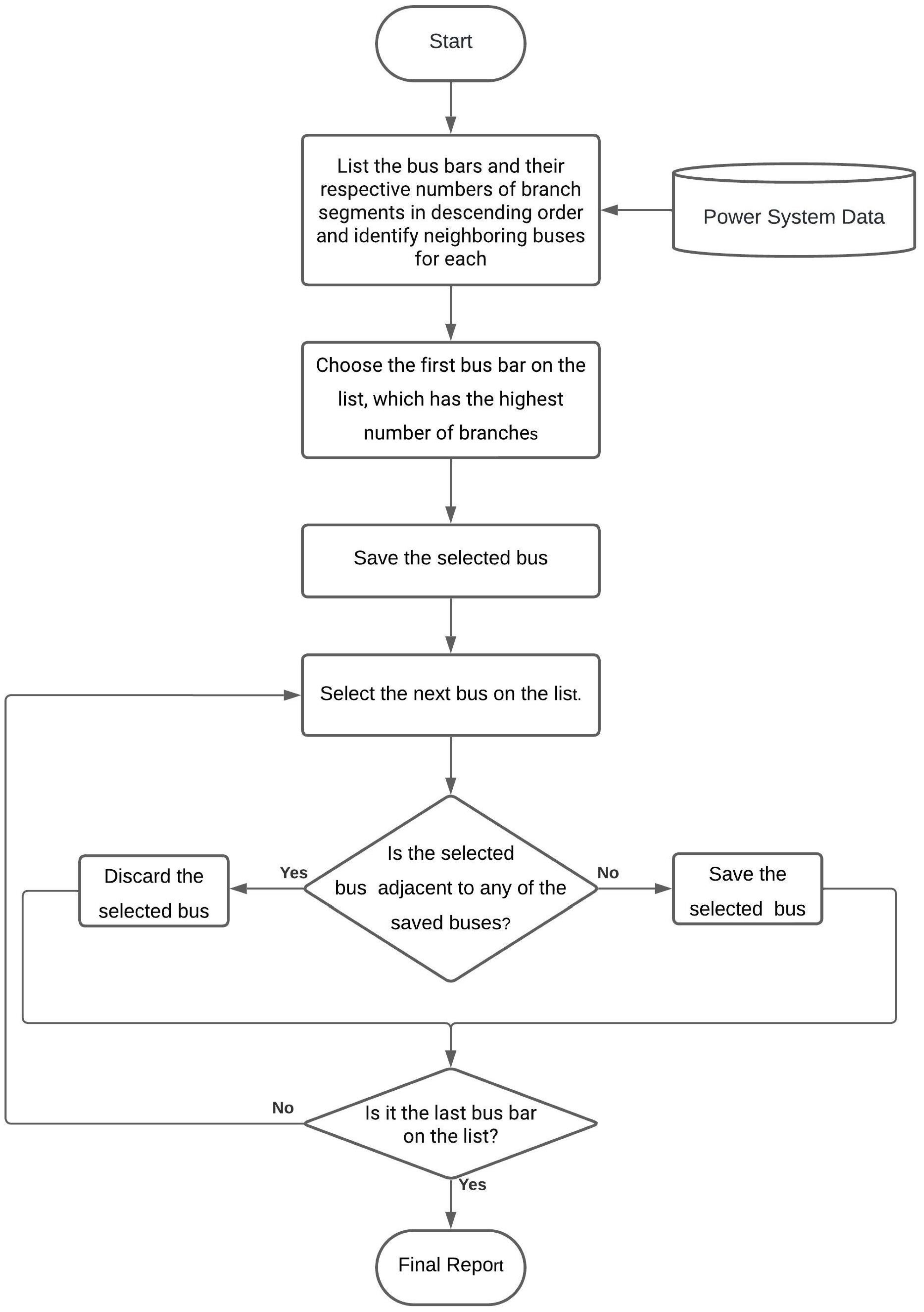
In this sense, as a continuation of the previous work, the authors expand the application of Jaya algorithm for harmonic state and power flow estimation for larger systems. The methodology specifically targets IEEE 14-bus and IEEE 30-bus systems, aiming to demonstrate the effectiveness and efficiency of the Jaya algorithm in resolving harmonic estimation challenges. Results are compared with those obtained using ESs, chosen as a benchmark due to their proven effectiveness in HSE, supported by empirically fine-tuned numerous parameters, contrasting with the fewer parameters of the Jaya methodology. This comparison will assess the algorithms’ efficacy in terms of accuracy and processing time. Furthermore, the authors also present a strategic approach for the allocation of PQ meters in power systems, based on the number of branches at each bus and their proximity, aiming to cover the fewest possible buses while maintaining system observability for power flow estimation and HSE.

2. Evolutionary Strategies

Evolutionary Strategies (ESs) are an optimization technique inspired by evolutionary principles, originally developed by Ingo Rechenberg and Hans-Paul Schwefel in the 1960s and 1970s [20,21,22,23], with subsequent refinements and developments proposed in later works [24]. These strategies were initially conceived as a way to mimic natural evolution processes in the context of solving complex engineering problems. In ESs, a population of potential solutions, represented by individuals, undergoes iterative improvement through genetic mutations and recombination. Mutations introduce variations in individual solutions by altering their parameters, while recombination allows the exchange of information between individuals to generate potentially better solutions. The fitness of each individual is evaluated based on its proximity to the optimal solution, driving the selection of individuals for the next generation. This iterative cycle continues until a predefined stopping criterion is met, such as achieving an acceptable level of solution quality or completing a maximum number of generations.

At the end of each generation, a selection process takes place where the fittest individuals—those closest to the optimal solution—are chosen to form the next generation. This cycle of mutation, recombination, and selection continues until a stopping criterion is met, which could be a predefined number of generations or the attainment of an acceptable solution.

Briefly, an evolutionary algorithm can be described as follows [25]:

  1:

$t\leftarrow 0;$

  2:

initialize $P\left(t\right);$

  3:

evaluate $P\left(t\right);$

  4:

while (stopping criterion) do

  5:      

$P^{\prime }\left(t\right)\leftarrow$ variation $P\left(t\right);$

  6:      

evaluate $P^{\prime }\left(t\right);$

  7:      

$Q\left(t\right)=f\left(P\right(t\left)\right);$

  8:      

$P(t+1)\leftarrow$ selection $[P^{\prime }\left(t\right)\cup P\left(t\right)];$

  9:      

$t\leftarrow t+1;$

10:

end while

In this context, $P\left(t\right)$ represents a population with $\mu$ individuals. $P^{\prime }\left(t\right)$ denotes a set of $\lambda$ individuals generated through recombination and mutation from $P\left(t\right)$. $Q\left(t\right)$ is a function of $P\left(t\right)$ and can be zero or equal to $P\left(t\right)$. During the evaluation phase, each individual is scored based on its distance from the optimal solution. The best-performing individuals are then selected to form the initial population for the next generation. This iterative process continues until the stopping criterion is satisfied. The basic flowchart of the ES algorithm is shown in Figure 1.

Figure 1. Basic flowchart of the ES algorithm.

3. Jaya Algorithm

3.1. Introduction

The Jaya algorithm, developed by [26], is a groundbreaking methodology in the field of mathematical optimization, distinguished by its simplicity and efficiency. Unlike many other optimization algorithms, Jaya requires only a few specific parameters for its operation, significantly reducing the complexity of its implementation and tuning.

The core principle of the Jaya algorithm is to steer solutions towards the best solution obtained so far, while simultaneously moving them away from the worst solution observed within the solution population. This “directional search” approach enables rapid convergence to an optimal or near-optimal solution, without the need for crossover or mutation operators typical of other optimization algorithms, such as genetic algorithms and Evolutionary Strategies.

The effectiveness and versatility of the Jaya algorithm have been demonstrated in various studies and applications, addressing complex optimization problems across different engineering fields [27]. The Jaya algorithm has shown great promise in solving power flow problems in electric power systems, particularly noted for its optimization capability without the need for tuning specific parameters. In a study conducted by [28], the Jaya algorithm proved effective in optimizing power flow, producing optimal solutions with rapid convergence, and demonstrating superior performance compared to other stochastic algorithms in terms of the optimality and feasibility of the proposed solutions. This research underscores the applicability of the Jaya algorithm in obtaining efficient and viable solutions for complex power flow problems.

A significant innovation was introduced by [17] with the development of the modified quasi-oppositional Jaya (QOMJaya) algorithm to solve multi-objective optimal power flow (MOOPF) problems. This method enhances convergence properties, exploration capabilities, and solution optimality by incorporating a learning strategy based on quasi-opposition.

Additionally, [29] proposed a hybrid Jaya–Powell’s Pattern Search approach to solve the multi-objective optimal power flow problem, integrating the Jaya algorithm for exploration and Powell’s Pattern Search method for exploitation.

However, considering the absence in the current literature of any applications of the Jaya algorithm in the HSE of electric power systems, the canonical version of Jaya as presented by Rao in 2016 will be applied.

3.2. Basic Equation

The basic update equation in the Jaya algorithm for optimizing a problem is given by [27]

$$X_{i,j}^{\left(new\right)}=X_{i,j}+r_1·(X_{best,j}-\left|X_{i,j}\right|)-r_2·(X_{worst,j}-\left|X_{i,j}\right|)$$

(1)

where $X_{i,j}^{\left(new\right)}$ is the new value of the $j\mathrm{th}$ variable for the $i\mathrm{th}$ candidate solution in the next iteration, $X_{i,j}$ is the current value of the $j\mathrm{th}$ variable for the $i\mathrm{th}$ candidate solution, $X_{best,j}$ is the value of the $j\mathrm{th}$ variable for the best candidate solution in the current population, $X_{worst,j}$ is the value of the $j\mathrm{th}$ variable for the worst candidate solution in the current population, and $r_1$ and $r_2$ are random numbers generated within the range [0, 1] for each iteration and each variable, providing stochastic elements to the update mechanism.

This equation is used to update each variable of each candidate solution in the population. The idea is to move the current solution towards the best solution and away from the worst solution, thereby iteratively improving the quality of solutions in the population.

3.3. Process Overview

As shown in Figure 2, the Jaya algorithm begins with initialization and initial settings, where a population of solutions is randomly generated within the search space. Following this is the evaluation step, where each solution is assessed based on the problem’s objective function, and the best and worst solutions in the population are identified, crucial for the subsequent steps. The update step uses Equation (1) to adjust each solution, propelling them towards the best solution and distancing them from the worst. This process is repeated in a loop, where after each update, the solutions are reevaluated, and the best and worst are identified again. The loop continues until a stopping criterion is satisfied, such as reaching the maximum number of iterations or a specified convergence condition [26]. The flowchart ends when the algorithm presents the best solution found as the result.

Figure 2. Flowchart of the basic Jaya method.

4. Problem Formulation

4.1. General Scheme

Firstly, the harmonic orders of interest are defined, and the admittance matrices for the fundamental frequency and harmonic frequencies are calculated from the power system data. Considering that the methodology proposed in this work aims to estimate power flow and HSE by assessing harmonic voltage distortion levels at buses without direct measurements, it is assumed that measurements are available only at select buses in the power system. These measured values serve as a database for estimating fundamental and harmonic frequency values at buses without direct measurements. The analysis and estimation of data for the fundamental frequency and each harmonic order will be conducted separately, employing either the Jaya algorithm or Evolutionary Strategies. Finally, by comparing the measured and estimated voltage values for the fundamental frequency and harmonic orders, the Total Harmonic Distortion (THD) can be determined. The proposed methodology is illustrated by the block diagram shown in Figure 3.

Figure 3. Block diagram for the proposed methodology.

4.2. Reference Values

PQ meters installed at selected buses of the system deliver synchronized reference data for current and voltage, including magnitude and phase values, across the harmonic orders of interest as well as the fundamental frequency.

4.3. Harmonic Orders of Interest

The determination of which harmonic orders to examine is influenced by the availability of PQ meters and the specific objectives of the research. In this particular study, the emphasis is placed on identifying and analyzing the most frequently encountered harmonics in power systems. This includes the odd harmonic orders 3, 5, 7, 9, 11, and 13, which are often most significant in terms of their impact on system performance and equipment [30], enabling the calculation, from the values at the fundamental frequency, of the THD given by

$$\mathrm{THD}={\displaystyle \frac{\sqrt{{\sum }_{h=2}^n{V}_h^2}}{V_1}}$$

(2)

where THD represents the Total Harmonic Distortion, $V_h$ signifies the magnitude of the $h\mathrm{th}$ harmonic component, $V_1$ denotes the magnitude of the fundamental component, and n represents the last harmonic component considered in the summation.

4.4. Individual Representation

In the HSE study, each individual represents a potential solution, embodying a possible state of the system. To address the study’s objectives effectively, it is essential to identify a distinct individual for each specific harmonic order h. This individual is responsible for representing the optimal solution for the system at that particular harmonic order. In this context, for a system consisting of t buses and m meters, and using the Jaya algorithm for optimization, each individual is represented by a matrix of $(t-m)$ rows and two columns.

Taking the IEEE 14-bus system as an example, the representation of an individual for Jaya is defined according to the expression in Equation (3). In this specific case, monitoring is limited to buses 2, 3, 8, 9, 12, and 14. The matrix columns, first and second, represent the magnitudes and phases of the voltages at each bus for the harmonic order h under analysis, respectively.

$${\mathrm{Individual}}_h=\left[\begin{array}{cc}{V}_h^2& {\theta }_h^2\\ V_h^3& {\theta }_h^3\\ V_h^5& {\theta }_h^5\\ V_h^7& {\theta }_h^7\\ V_h^9& {\theta }_h^9\\ V_h^{11}& {\theta }_h^{11}\\ V_h^{12}& {\theta }_h^{12}\\ V_h^{13}& {\theta }_h^{13}\end{array}\right]$$

(3)

where $V_h^i$ denotes the absolute voltage at bus i in harmonic order h; ${\theta }_h^i$ indicates the phase of voltage at bus i in harmonic order h.

However, within the context of the ES methodology, an additional column is appended for each variable, considering that it is imperative to account for mutation steps aligned with the magnitudes and phases of voltages, thus necessitating the addition of two columns in this instance. As an illustrative example, the representation of an individual for the IEEE 14-bus network is defined as shown in (4), where measurements are taken exclusively at buses 1, 4, 6, 8, 10, and 14. The first and third columns represent the magnitudes and phases of voltage at each bus and harmonic order h, while the second and fourth columns denote the mutation steps.

$${\mathrm{Individual}}_h=\left[\begin{array}{cccc}{V}_h^2& {\sigma }_{V,h}^2& {\theta }_h^2& {\sigma }_{\theta ,h}^2\\ V_h^3& {\sigma }_{V,h}^3& {\theta }_h^3& {\sigma }_{\theta ,h}^3\\ V_h^5& {\sigma }_{V,h}^5& {\theta }_h^5& {\sigma }_{\theta ,h}^5\\ V_h^7& {\sigma }_{V,h}^7& {\theta }_h^7& {\sigma }_{\theta ,h}^7\\ V_h^9& {\sigma }_{V,h}^9& {\theta }_h^9& {\sigma }_{\theta ,h}^9\\ V_h^{11}& {\sigma }_{V,h}^{11}& {\theta }_h^{11}& {\sigma }_{\theta ,h}^{11}\\ V_h^{12}& {\sigma }_{V,h}^{12}& {\theta }_h^{12}& {\sigma }_{\theta ,h}^{12}\\ V_h^{13}& {\sigma }_{V,h}^{13}& {\theta }_h^{13}& {\sigma }_{\theta ,h}^{13}\end{array}\right],$$

(4)

where $V_h^i$ denotes the absolute voltage at bus i in harmonic order h; ${\theta }_h^i$ indicates the phase of voltage at bus i in harmonic order h; ${\sigma }_{V,h}^i$ represents the mutation step for the voltage parameter at bus i in harmonic order h (not applicable to the Jaya algorithm); and ${\sigma }_{\theta ,h}^i$ signifies the mutation step for the phase parameter at bus i in harmonic order h (not applicable to the Jaya algorithm).

4.5. State Estimation for Each Harmonic of Interest

In the HSE process, following the selection of harmonic orders considered relevant for this study and the definition of individual representation, each is subjected to the state estimation algorithm proposed in this work, which is based on the Jaya algorithm or ES algorithm. The input data for the algorithm not only include the selected harmonic orders but also actual measurements of voltages and currents, coupled with the system’s admittance matrix. The execution of the algorithm for each harmonic of interest is meticulously carried out, and the results are compiled into a final report.

4.6. Evaluation

The evaluation process is designed to determine the fitness of each individual by quantifying how closely each solution approximates the established reference values. In this context, each individual is considered a potential solution to the HSE problem. Thus, for each harmonic order h selected for analysis, the voltage vector corresponding to each individual, combined with the system’s admittance matrix, results in the formulation of an estimated current vector $I_h^i$, as illustrated by

$$I_h^i=\sum _{j=1}^{nb}{Y}_h^{ij}{V}_h^j$$

(5)

where $V_h^j$ is the voltage at bus j, harmonic order h, $Y_h^{ij}$ is the element $\left(ij\right)$ of the admittance matrix at the frequency for harmonic order h, and $nb$ is the number of monitored buses.

The accuracy of these estimates is verified by calculating the difference between the estimated current vector and the measured current vector $I_{hM}^i$, a process that generates the error vector $e{e}_i^h$, as shown by

$$e{e}_h^i=|I_h^i-I_{hM}^i|$$

(6)

where $e{e}_i^h$ is the estimation error at bus i, harmonic order h, $I_h^i$ is the calculated current at bus i from an individual who represents the voltages at the buses for selected harmonic orders, and $I_{hM}^i$ is the measured current, harmonic order h at bus i. This error vector quantitatively represents the discrepancy between the estimated condition and the actual system condition, providing a crucial metric for performance evaluation. After calculating the errors for all monitored buses, the fitness of each individual analyzed for the specified harmonic order is calculated as the inverse of the sum of the squares of the error vector elements, as defined by

$$Fitnes{s}_h={\displaystyle \frac{1}{{\sum }_{i=1}^{nb}{\left(e{e}_h^i\right)}^2}}$$

(7)

where ${\mathit{Fitness}}_h$ is the individual fitness at harmonic order h.

4.7. Selection

In the case of the ES methodology, the selection is deterministic, ensuring that only the fittest individuals, i.e., those with the highest fitness, are chosen while maintaining a constant population size from generation to generation. Selection includes both parents and offspring to allow for elitism, ensuring that the best parent individuals are preserved throughout generations.

On the other hand, the Jaya algorithm methodology employs a unique selection methodology within its iterative process, as detailed in Figure 2. Originating from an initial population generated randomly within the search space, each individual in the population automatically generates a successor using the Equation (1). This successor then undergoes a fitness evaluation, where its fitness is compared to that of its progenitor. If the successor’s fitness surpasses that of its originator, it replaces the latter in the population; otherwise, it is discarded, thus optimizing the process by focusing resources on more promising candidates.

Furthermore, the Jaya algorithm identifies the best and worst individuals within the population throughout all iterations. The best individuals are those who consistently demonstrate the highest levels of fitness, effectively guiding the search toward more optimal solutions. On the other hand, the worst individuals represent the lowest levels of fitness, serving as benchmarks for the necessary improvements and adjustments in the algorithm’s search dynamics. Once the stopping criterion is met, the best solution for each harmonic order is considered the final solution for that specific harmonic order.

5. Application

5.1. Initial Considerations

In this work, the IEEE 14-bus and IEEE 30-bus systems were selected for the application of the proposed HSE methodology and are illustrated in Figure 4 and Figure 5, whose parameters and other information are obtained from [31,32], respectively. More informations can be found in Appendix A. The choice of these specific systems stems from their established usage in power system studies, offering a balance between complexity and manageability. Additionally, the availability of test data and widespread use in academic research make them suitable candidates for validating the proposed methodology.

Initially, both systems were simulated using PSCAD X4 software (version 4.5.0.0) at the fundamental frequency to validate the data. Since the operating conditions at the fundamental frequency considered in this study are the same as those of the official test models, the power flow results could be validated through [33,34] for the IEEE 14-bus and IEEE 30-bus systems, respectively.

Subsequently, both systems were simulated using the PSCAD software in a scenario featuring multiple harmonic sources of orders 3, 5, 7, 9, 11, and 13, which were randomly distributed.

Figure 4. IEEE 14-bus system (adapted from [31]).

The power flow at the fundamental frequency and the harmonic state of the studied systems at all buses, including the values of current and voltage harmonic orders of interest, were obtained from PSCAD software and are provided in Appendix B.

Figure 5. IEEE 30-bus system (adapted from [35]).

5.2. PQ Meters Allocation

The initial and fundamental step in the HSE methodology is to determine the minimum number and optimal locations of buses that need to be monitored to ensure system observability.

One of the selection criteria for measurement points involves considering the number of line segments connected to each bus. Buses with a higher number of connections are prioritized for measurement inclusion. Additionally, it is crucial to avoid selecting adjacent buses. This approach is based on the premise that voltages at neighboring buses can be estimated if one of them is already measured, thus minimizing the total number of PQ meters required.

To effectively select these buses, a comprehensive strategy was developed. This strategy, illustrated in the flowchart in Figure 6, involves several steps. First, all buses are mapped and the number of line segments branching from each bus is counted. Then, the buses are listed in descending order according to the number of branches. This hierarchical listing allows for prioritizing buses with the highest connectivity for measurement inclusion.

Figure 6. Flowchart of the meter allocation method presented.

The strategy also incorporates a method to systematically check for adjacency, ensuring that directly connected neighboring buses are not selected consecutively. This step is crucial for maintaining the efficiency of the measurement system and reducing redundancy.

Moreover, the flowchart incorporates an iterative process to re-evaluate and adjust the selection as required. This ensures that the final group of selected buses offers comprehensive observability of the system with minimal PQ meters. Implementing this approach enhances the efficiency and effectiveness of the HSE process, resulting in improved accuracy and reliability in HSE.

The mapping results for the IEEE 14-bus system are presented in Table 1. According to the adopted strategy, monitoring is required for 6 specific buses: buses 1, 4, 6, 8, 10, and 14.

Table 1. List of buses, number of connections, and neighboring buses for the IEEE 14-bus system.

Bus	Connections	Neighbors
4	5	2, 3, 5, 7, 9
2	4	1, 3, 4, 5
5	4	1, 2, 4, 6
6	4	5, 11, 12, 13
9	4	4, 7, 10, 14
7	3	4, 8, 9
13	3	6, 12, 14
1	2	2, 5
3	2	2, 4
10	2	9, 11
11	2	6, 10
12	2	6, 13
14	2	9, 13
8	1	7

For the IEEE 30-bus system, the mapping yielded Table 2, and the adopted strategy resulted in the selection of 12 buses for comprehensive monitoring. Specifically, the chosen buses are buses 3, 5, 6, 11, 12, 17, 18, 20, 21, 24, 26, and 27. This strategic approach ensures extensive and effective coverage, enabling detailed and accurate observation of harmonic states across different sections of the system.

Table 2. List of buses, number of connections, and neighboring buses for the IEEE 30-bus system.

Bus	Connections	Neighbors
6	7	2, 4, 7, 8, 9, 10, 28
10	6	6, 9, 17, 20, 21, 22
12	5	4, 13, 14, 15, 16
2	4	1, 4, 5, 6
4	4	2, 3, 6, 12
15	4	12, 14, 18, 23
27	4	25, 28, 29, 30
9	3	6, 10, 11
22	3	10, 21, 24
24	3	22, 23, 25
25	3	24, 26, 27
28	3	6, 8, 27
1	2	2, 3
3	2	1, 4
5	2	2, 7
7	2	5, 6
8	2	6, 28
14	2	12, 15
16	2	12, 17
17	2	10, 16
18	2	15, 19
19	2	18, 20
20	2	10, 19
21	2	10, 22
23	2	15, 24
29	2	27, 30
30	2	27, 29
11	1	9
13	1	12
26	1	25

5.3. ES Methodology Tuning

Table 3 presents the various parameters considered characteristic of an algorithm based on ES. These values were empirically obtained, aiming for convergence in the shortest possible time and accuracy of estimated values.

Table 3. Parameters for Evolutionary Strategy methodology.

Parameter	Value for IEEE 14-Bus	Value for IEEE 30-Bus
Maximum number of generations	2000	2000
Number of individuals in the initial population	40	150
Mutation operations per individual	5	5
Recombination rate	10%	20%
Initial mutation step for voltage magnitudes	1	1
Initial mutation step for voltage phase	${\displaystyle \frac{2\pi }{3}}$	${\displaystyle \frac{2\pi }{3}}$
Self-adaptation parameter $\beta$	5	5

5.4. Jaya Algorithm Tuning

Given that the Jaya algorithm in its original form includes only two parameters—the number of individuals in the initial population and the number of generations—these parameters were selected empirically. For the IEEE 14-bus system, the number of individuals in the initial population was set at 50, and the maximum number of generations was set at 2000. However, for the IEEE 30-bus system, these parameters were set at 150 and 5000, respectively, as listed in Table 4.

Table 4. Parameters for Jaya.

Parameter	Value for IEEE 14-Bus	Value for IEEE 30-Bus
Maximum number of generations	2000	5000
Number of individuals in the initial population	50	150

The stopping criterion was defined as either reaching the maximum number of generations or the stabilization of the fitness of the best individual, whichever occurs first. In this study, stabilization is determined when the fitness of the best individual remains unchanged for 10% of the maximum number of generations.

5.5. Implementation

The methodologies were implemented using the Python programming language, incorporating specific routines for computing the admittance matrix across various harmonic orders, reading reference values, and performing HSE using ES methodology and the Jaya algorithm.

6. Results and Discussion

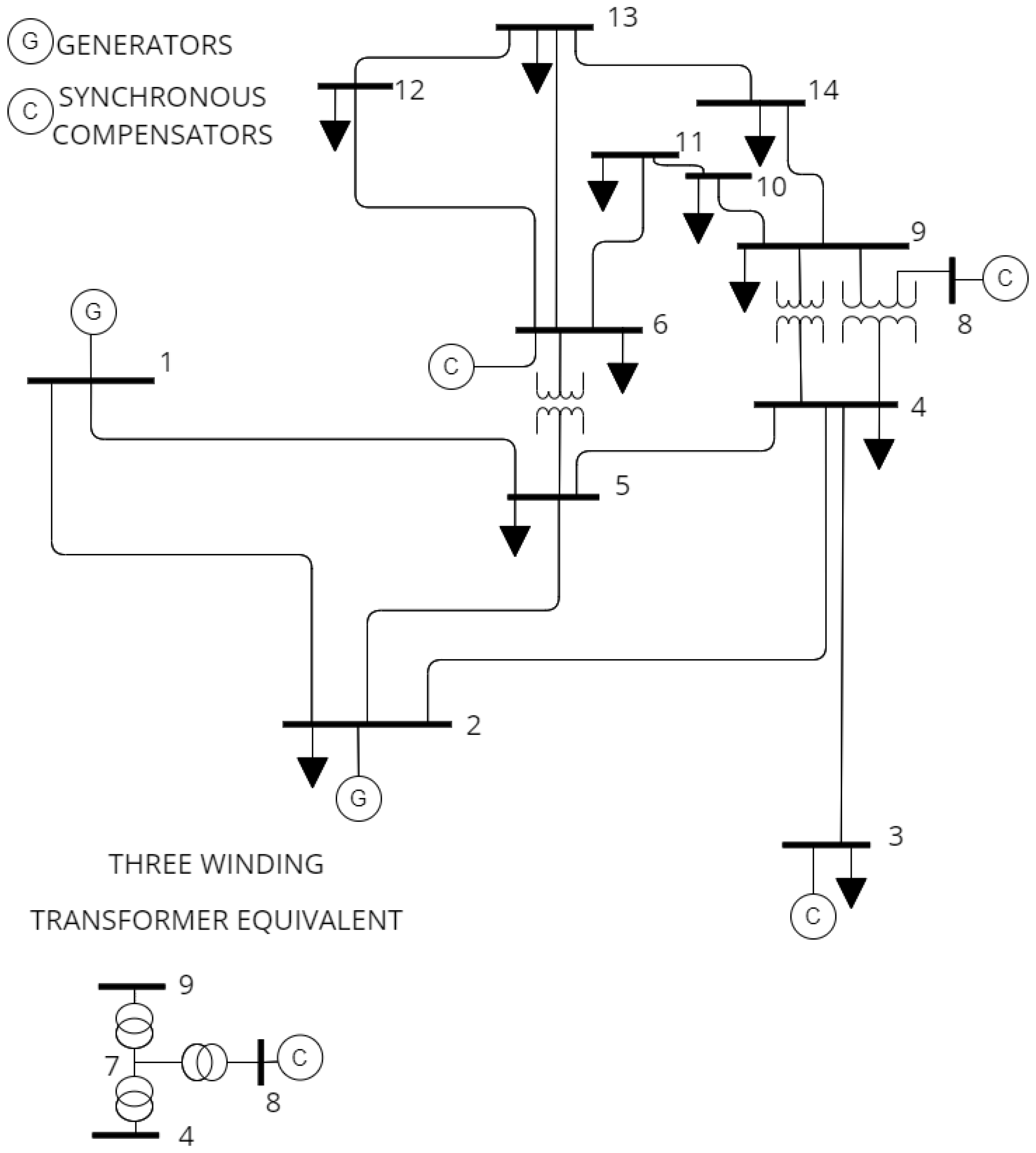
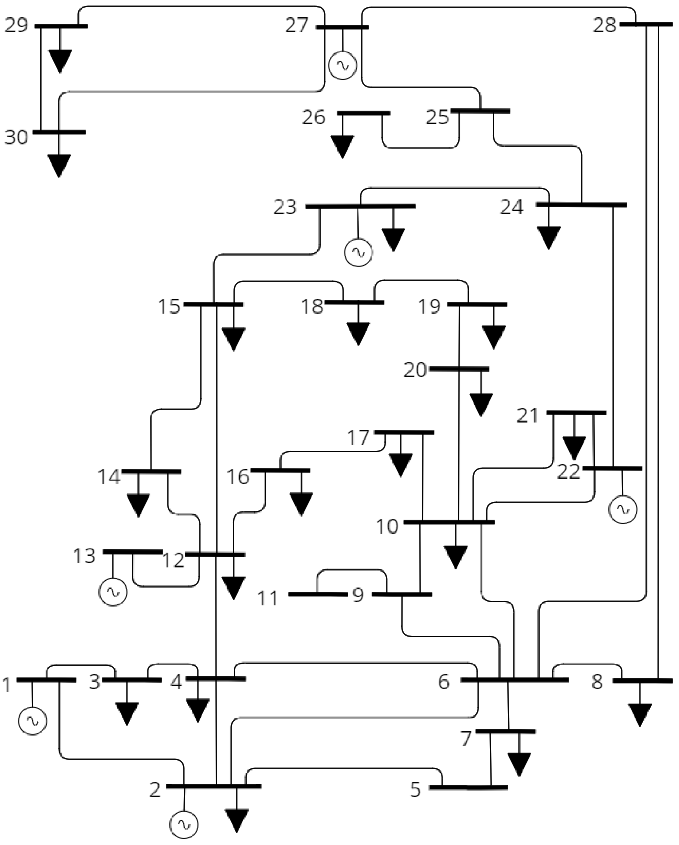
Considering the premises previously presented, the proposed methodology was applied to the IEEE 14-bus and IEEE 30-bus systems using the proposed Jaya algorithm as well as the ES algorithm for a comparative study between the two methodologies.

Thus, the analysis involved the introduction of harmonic currents of order 3, 5, 7, 9, 11, and 13 in some buses, causing harmonic distortion in the system. This scenario presents a challenge for the system operator to identify these sources, considering a hypothetical situation where the operator is unaware of these sources and does not have PQ meters throughout the system.

As discussed, the ES algorithm required empirical tuning of various input parameters, which became a daunting task as the parameters are sensitive to each other. This necessitated running the codes multiple times to find suitable parameter tuning, a situation that is exacerbated when dealing with different problems, requiring specific parameters tuned for each analysis situation. This tuning is performed to allow both the diversity of the initial population of possible solutions and the rapid convergence to a global optimum. Conversely, the Jaya algorithm does not allow parameter adjustment freedom, containing only two parameters, namely the initial population size and the maximum number of generations, making it very simple and easy to tune.

With the initial parameters defined, based on voltage measurements at some selected buses, the algorithm receives system data, only the measured values at these buses and the initial parameters, and estimates the voltage amplitudes and phases at unmonitored buses for the fundamental frequency and the harmonic orders of interest.

To demonstrate that the voltage estimation errors are consistently kept within a minimal value range for each harmonic order, the proposed HSE methodology was executed 30 times, first applying the ES algorithm and then the Jaya algorithm, obtaining the results for each fundamental and harmonic order of interest at unmonitored buses. This allows us to obtain the THD and compare the time and consequently the processing cost for both algorithms. The results are presented and discussed below.

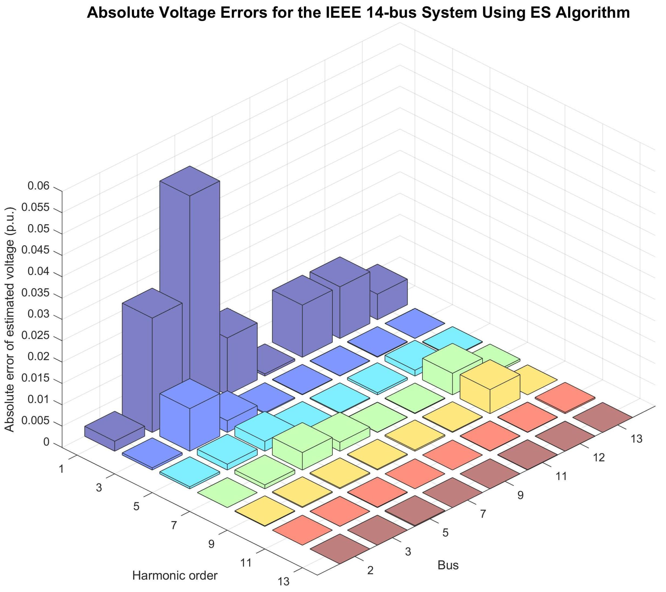
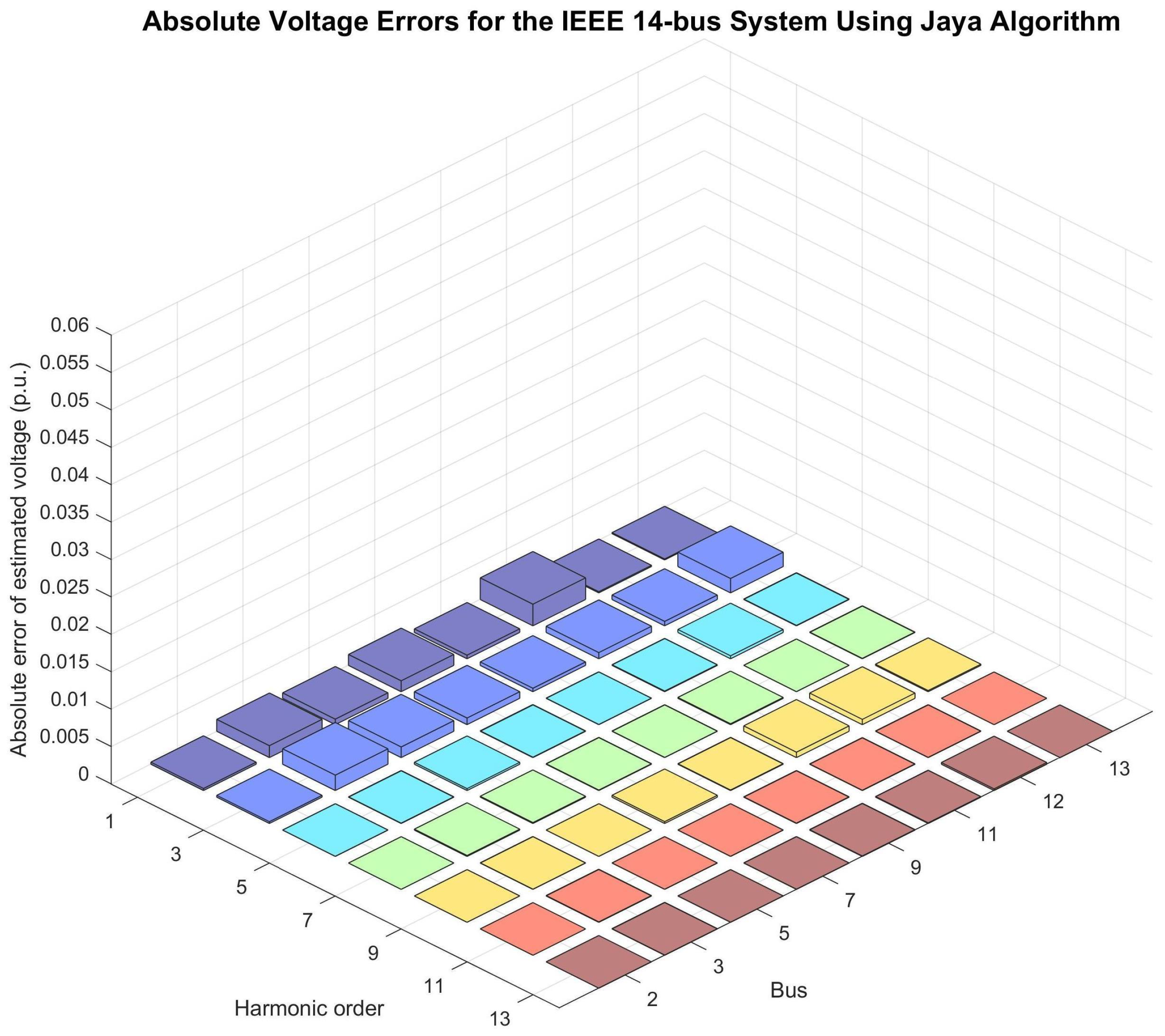
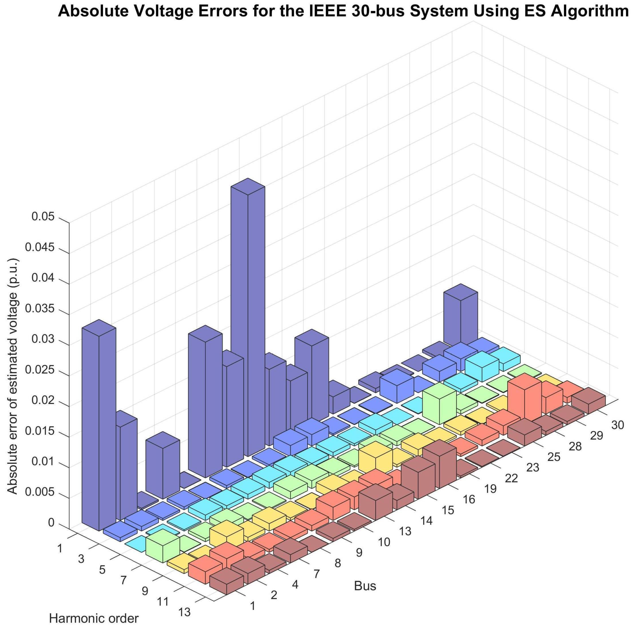
Considering that the amplitudes of the harmonic orders can be reasonably small and that any slight difference would result in considerable relative errors, the approach was to address the absolute errors between the estimated and real values, which allows for better analysis of the results. The average absolute errors of the obtained voltage magnitudes are presented in Table 5 and Table 6 using the ES and Jaya methodologies, respectively, for the IEEE 14-bus system, and in Table 7 and Table 8 using the ES and Jaya methodologies, respectively, for the IEEE 30-bus system. The same results are presented graphically in Figure 7 and Figure 8 for the IEEE 14-bus system and in Figure 9 and Figure 10 for the IEEE 30-bus system. Considering the estimates for the fundamental frequency, it is observed that the highest errors obtained using ES were 0.051 p.u. and 0.043 p.u. for the IEEE 14-bus and IEEE 30-bus systems, respectively, higher than the errors obtained with the Jaya algorithm, which were 0.003 p.u. and 0.011 p.u. for the two systems, respectively, demonstrating the efficiency of the Jaya algorithm for power flow estimation. For the harmonic components, considering the IEEE 14-bus system, the highest errors obtained are 0.010 p.u. using ES and 0.002 p.u. using Jaya, both in the third harmonic. In the case of the IEEE 30-bus system, the highest errors are 0.006 p.u. using ES and 0.007 p.u. using Jaya, both in the eleventh harmonic, which may be an insignificant difference with little impact on the THD estimation, as it is a higher-order harmonic whose magnitudes, in this case, are smaller than those of lower-order harmonics. Thus, the errors obtained with the Jaya algorithm, which are comparable or lower to those obtained with the ES algorithm for the harmonic components, demonstrate the effectiveness of the HSE using the proposed methodology based on the Jaya algorithm.

Table 5. Absolute errors of estimated voltage (p.u.) for the IEEE 14-bus system using ES algorithm.

Bus	Harmonic Order
	1	3	5	7	9	11	13
2	0.002	0.001	0.000	0.000	0.000	0.000	0.000
3	0.027	0.010	0.001	0.001	0.000	0.000	0.000
5	0.051	0.003	0.002	0.004	0.000	0.000	0.000
7	0.013	0.000	0.000	0.002	0.000	0.000	0.000
9	0.001	0.000	0.000	0.000	0.000	0.000	0.000
11	0.012	0.000	0.000	0.000	0.000	0.000	0.000
12	0.012	0.000	0.001	0.005	0.006	0.000	0.000
13	0.006	0.000	0.000	0.000	0.000	0.000	0.000
Maximum Error	0.051	0.010	0.002	0.005	0.006	0.000	0.000

Table 6. Absolute errors of estimated voltage (p.u.) for the IEEE 14-bus system using Jaya algorithm.

Bus	Harmonic Order
	1	3	5	7	9	11	13
2	0.000	0.000	0.000	0.000	0.000	0.000	0.000
3	0.002	0.002	0.000	0.000	0.000	0.000	0.000
5	0.001	0.001	0.000	0.000	0.000	0.000	0.000
7	0.001	0.001	0.000	0.000	0.000	0.000	0.000
9	0.000	0.000	0.000	0.000	0.000	0.000	0.000
11	0.003	0.001	0.000	0.000	0.001	0.000	0.000
12	0.000	0.001	0.000	0.000	0.001	0.000	0.000
13	0.000	0.002	0.000	0.000	0.000	0.000	0.000
Maximum Error	0.003	0.002	0.000	0.000	0.001	0.000	0.000

Table 7. Absolute errors of estimated voltage (p.u.) for the IEEE 30-bus system using ES algorithm.

Bus	Harmonic Order
	1	3	5	7	9	11	13
1	0.032	0.001	0.000	0.003	0.001	0.002	0.002
2	0.015	0.001	0.000	0.000	0.000	0.002	0.002
4	0.000	0.000	0.000	0.000	0.003	0.001	0.001
7	0.008	0.000	0.001	0.001	0.001	0.000	0.001
8	0.000	0.000	0.001	0.000	0.001	0.001	0.000
9	0.022	0.000	0.001	0.000	0.000	0.001	0.001
10	0.016	0.000	0.001	0.001	0.000	0.002	0.000
13	0.043	0.000	0.001	0.001	0.001	0.002	0.003
14	0.013	0.002	0.001	0.001	0.000	0.002	0.002
15	0.009	0.002	0.001	0.000	0.003	0.000	0.004
16	0.013	0.000	0.000	0.001	0.000	0.001	0.005
19	0.003	0.000	0.001	0.001	0.001	0.001	0.000
22	0.000	0.000	0.000	0.000	0.000	0.000	0.000
23	0.001	0.003	0.000	0.004	0.001	0.001	0.000
25	0.000	0.000	0.000	0.001	0.000	0.002	0.002
28	0.000	0.002	0.001	0.000	0.000	0.006	0.001
29	0.000	0.002	0.002	0.000	0.001	0.003	0.001
30	0.008	0.001	0.001	0.000	0.000	0.001	0.002
Maximum Error	0.043	0.003	0.002	0.004	0.003	0.006	0.005

Table 8. Absolute errors of estimated voltage (p.u.) for the IEEE 30-bus system using Jaya algorithm.

Bus	Harmonic Order
	1	3	5	7	9	11	13
1	0.011	0.001	0.001	0.000	0.002	0.007	0.003
2	0.003	0.001	0.004	0.000	0.001	0.007	0.002
4	0.005	0.000	0.002	0.001	0.000	0.002	0.001
7	0.005	0.000	0.002	0.001	0.000	0.004	0.001
8	0.001	0.001	0.000	0.000	0.000	0.002	0.003
9	0.001	0.001	0.000	0.002	0.002	0.001	0.000
10	0.003	0.000	0.000	0.000	0.000	0.000	0.003
13	0.006	0.000	0.001	0.001	0.002	0.004	0.002
14	0.001	0.000	0.003	0.000	0.004	0.002	0.005
15	0.003	0.000	0.000	0.001	0.002	0.001	0.003
16	0.000	0.000	0.001	0.001	0.001	0.001	0.000
17	0.000	0.000	0.002	0.001	0.001	0.001	0.001
18	0.002	0.001	0.002	0.001	0.001	0.001	0.001
19	0.005	0.000	0.002	0.001	0.001	0.001	0.001
20	0.003	0.003	0.002	0.001	0.001	0.002	0.006
21	0.003	0.001	0.003	0.000	0.001	0.005	0.002
Maximum Error	0.011	0.003	0.004	0.002	0.004	0.007	0.006

Figure 7. Absolute voltage errors for each harmonic order and unmonitored bus for the IEEE 14-bus system using the ES algorithm.

Figure 8. Absolute voltage errors for each harmonic order and unmonitored bus for the IEEE 14-bus system using Jaya algorithm.

Figure 9. Absolute voltage errors for each harmonic order and unmonitored bus for the IEEE 30-bus system using the ES algorithm.

Figure 10. Absolute voltage errors for each harmonic order and unmonitored bus for the IEEE 30-bus system using the Jaya algorithm.

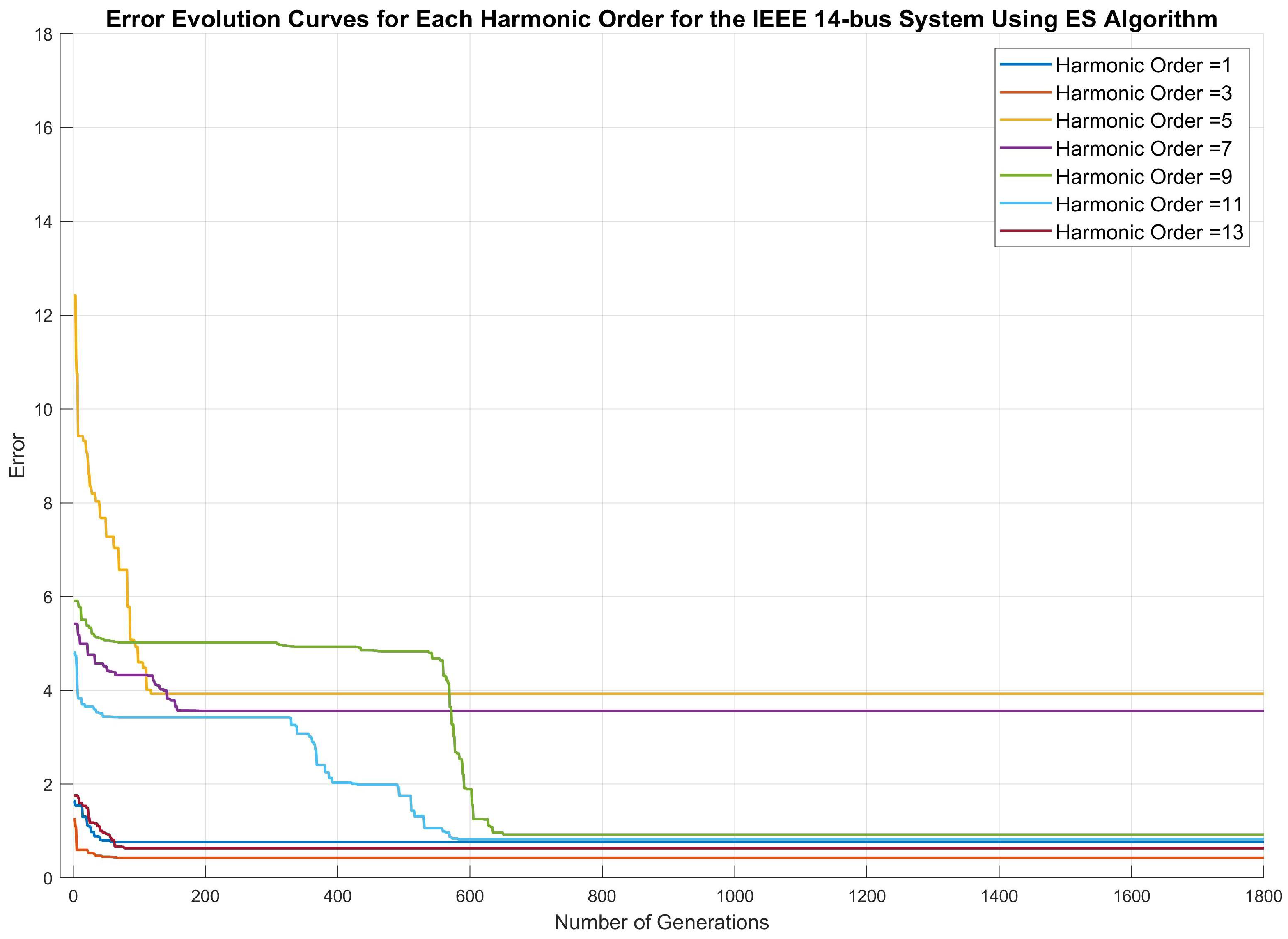
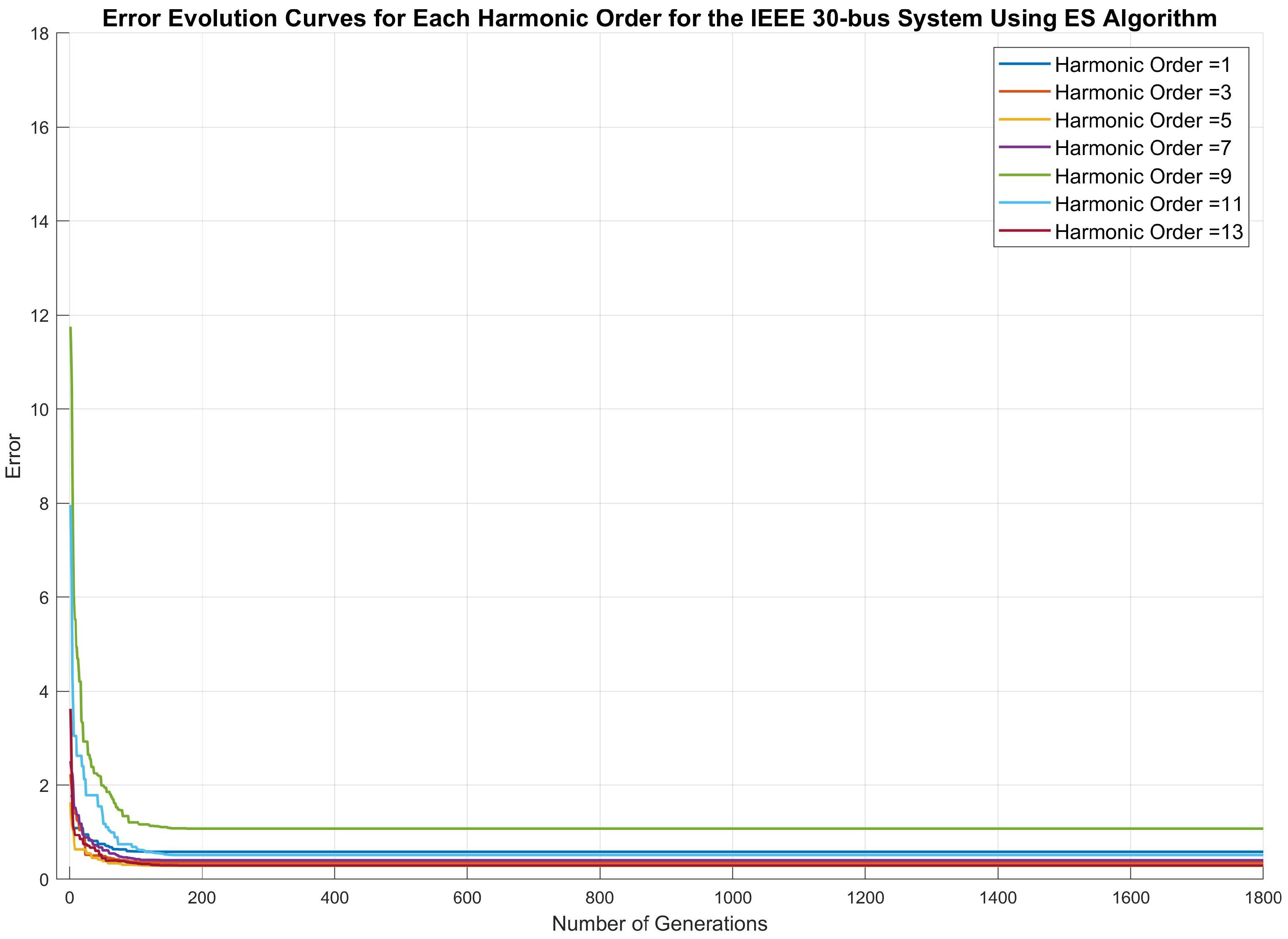
Considering the intrinsic characteristic of an evolutionary optimization algorithm like ES, which is based on selecting the fittest individuals to compose the initial population of the next generation, and an algorithm with few parameters like Jaya, which is directed by the best individual of each generation, the success in HSE is verified by the convergence of individuals or possible solutions to the optimal solution, that is, to the solution with the highest fitness and consequently the lowest error. In the present study, the lower error implies estimating the fundamental and harmonic components closer to the real values. To illustrate the error evolution curves’ behavior throughout the iterative process, Figure 11 and Figure 12 show the error evolution curves for the IEEE 14-bus network using, respectively, the ES and Jaya methodologies, and Figure 13 and Figure 14 show the error evolution curves for the IEEE 30-bus network using, respectively, the ES and Jaya methodologies. It is noted that the curves are raised for each harmonic order, considering that the algorithm is applied to each harmonic order at a time. The analysis of these curves allows us to conclude that they all move towards the lowest error plateau, stabilizing at certain values, proving the convergence of both methodologies. For harmonic frequencies, errors ranging from 0.000 to 0.061 p.u. for the IEEE 14-bus system and from 0.000 to 0.081 p.u. for the IEEE 30-bus system are observed. Some of the most significant error values are related to higher- and lower-order harmonics, whose impact on the total THD calculation is practically negligible. These errors for harmonic frequencies demonstrate that the algorithm is also effective in HSE.

Figure 11. Error evolution curves for each harmonic order for the IEEE 14-bus system using the ES algorithm.

Figure 12. Error evolution curves for each harmonic order for the IEEE 14-bus system using the Jaya algorithm.

Figure 13. Error evolution curves for each harmonic order for the IEEE 30-bus system using ES algorithm.

Figure 14. Error evolution curves for each harmonic order for the IEEE 30-bus system using the Jaya algorithm.

From the estimated voltage values for the fundamental frequency and harmonic orders at the unmonitored buses, the THD values at these buses are determined using Equation (2). These values are listed in Table 9 and Table 10 using the ES and Jaya methodologies, respectively, for the IEEE 14-bus system, and in Table 11 and Table 12 using the ES and Jaya methodologies, respectively, for the IEEE 30-bus system. 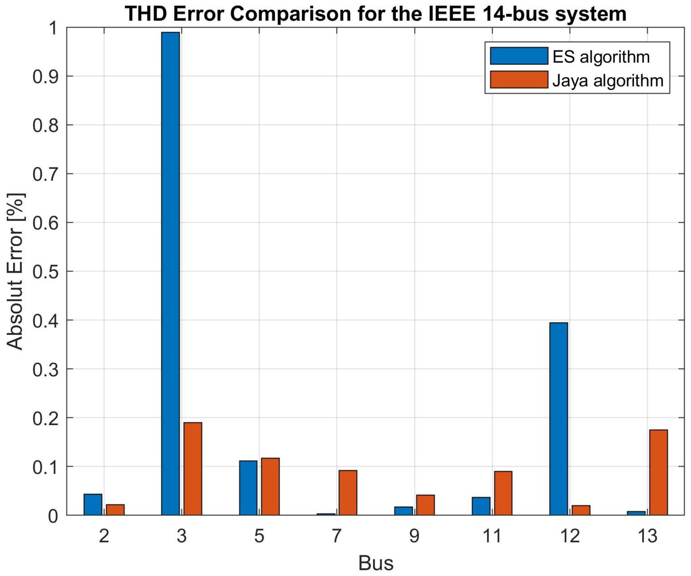The obtained THD error values for both methodologies are also illustrated in Figure 15 and Figure 16. It is observed that the THD errors for the IEEE 14-bus system are slightly higher for the ES algorithm, with a maximum error of 0.990% compared to 0.190% for the Jaya algorithm. However, for the IEEE 30-bus system, the Jaya algorithm resulted in a maximum error of 0.609%, which is slightly higher than the maximum error of 0.446% obtained with the ES algorithm, although the average error values are within the same range. Finally, the comparative analysis of these THD results allows for the conclusion that the Jaya algorithm is as effective as the ES algorithm by presenting average and maximum THD errors that are comparable to or better than those resulting from the ES algorithm. These errors are irrelevant for HSE, considering that the obtained results allow a comprehensive analysis of the systems for identifying the buses with the highest and lowest THD and consequently allowing the location of harmonic sources.

Table 9. Reference and estimated values of THD and their absolute errors for the IEEE 14-bus system using the ES algorithm.

Bus	Reference THD (%)	Estimated THD (%)	Error (%)
2	2.421	2.378	0.043
3	1.844	2.833	0.990
5	4.592	4.480	0.112
7	3.556	3.559	0.003
9	2.753	2.771	0.017
11	2.474	2.511	0.037
12	2.657	2.262	0.395
13	2.259	2.267	0.008
Maximum Error			0.990
Medium Error			0.115

Table 10. Reference and estimated values of THD and their absolute errors for the IEEE 14-bus system using the Jaya algorithm.

Bus	Reference THD (%)	Estimated THD (%)	Error (%)
2	2.421	2.443	0.022
3	1.844	2.034	0.190
5	4.592	4.475	0.117
7	3.556	3.464	0.092
9	2.753	2.795	0.042
11	2.474	2.564	0.090
12	2.657	2.677	0.020
13	2.259	2.434	0.175
Maximum Error			0.190
Medium Error			0.053

Table 11. Reference and estimated values of THD and their absolute errors for the IEEE 30-bus system using the ES algorithm.

Bus	Reference THD (%)	Estimated THD (%)	Error (%)
1	5.176	5.156	0.020
2	5.503	5.860	0.357
4	14.853	14.862	0.009
7	1.570	1.724	0.153
10	12.880	13.067	0.187
13	10.553	10.941	0.388
14	14.592	14.657	0.064
15	12.260	12.155	0.105
16	10.418	10.778	0.360
19	8.587	8.532	0.055
22	10.813	10.822	0.010
23	11.779	11.583	0.197
25	10.773	10.865	0.092
28	11.392	10.946	0.446
29	8.675	8.789	0.115
30	8.509	8.517	0.008
Maximum Error			0.446
Medium Error			0.095

Table 12. Reference and estimated values of THD and their absolute errors for the IEEE 30-bus system using the Jaya algorithm.

Bus	Reference THD (%)	Estimated THD (%)	Error (%)
1	5.176	5.532	0.355
2	5.503	4.894	0.609
4	14.853	15.057	0.204
7	1.570	1.886	0.316
10	12.880	12.908	0.028
13	10.553	10.355	0.198
14	14.592	14.767	0.174
15	12.260	12.446	0.186
16	10.418	10.689	0.271
19	8.587	8.658	0.071
22	10.813	10.783	0.030
23	11.779	11.718	0.061
25	10.773	10.882	0.109
28	11.392	11.466	0.074
29	8.675	8.477	0.198
30	8.509	8.333	0.176
Maximum Error			0.609
Medium Error			0.111

Figure 15. Comparison of THD errors between ES and Jaya methodologies for IEEE 14-bus system.

Figure 16. Comparison of THD errors between ES and Jaya methodologies for IEEE 30-bus system.

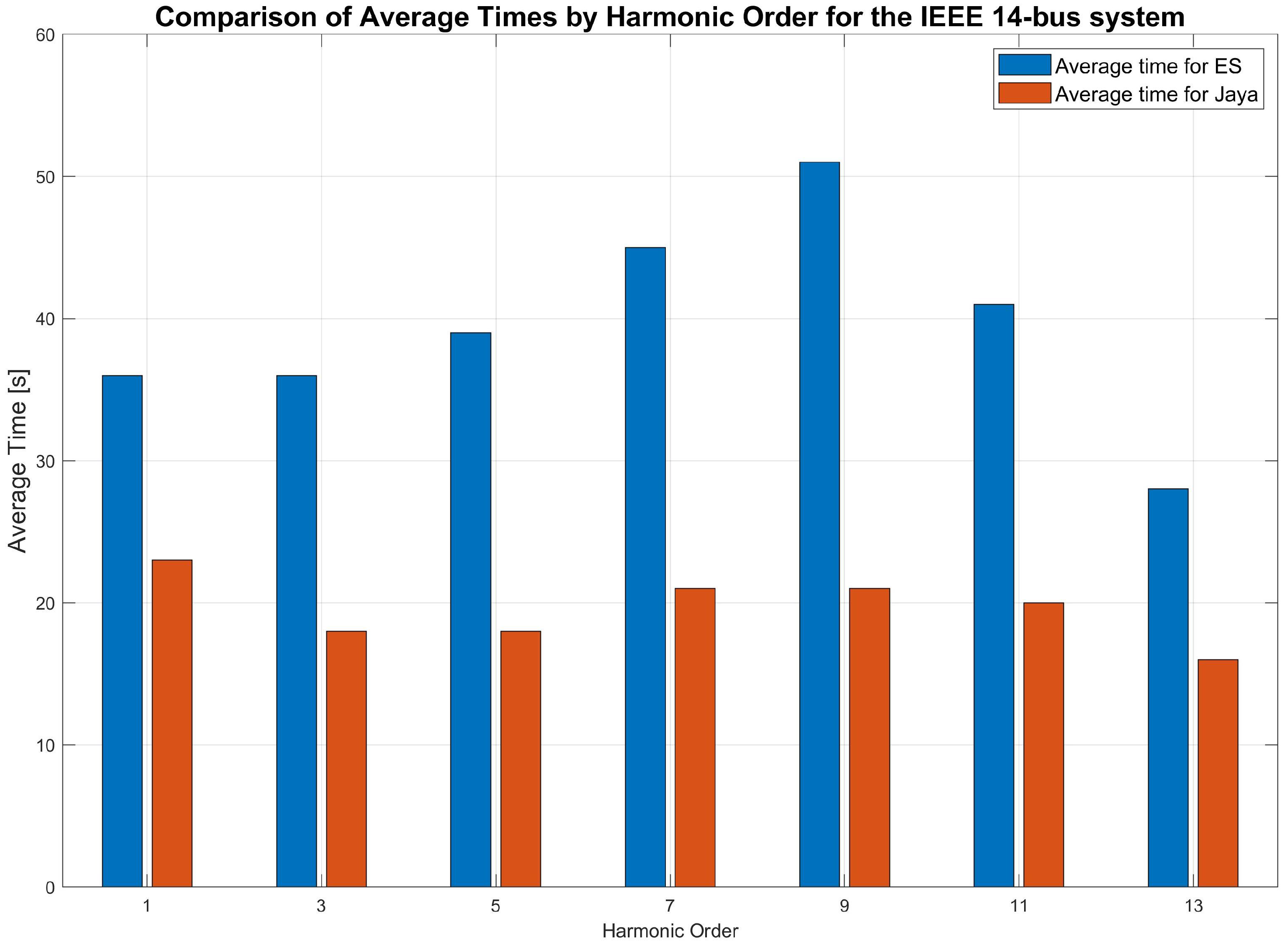
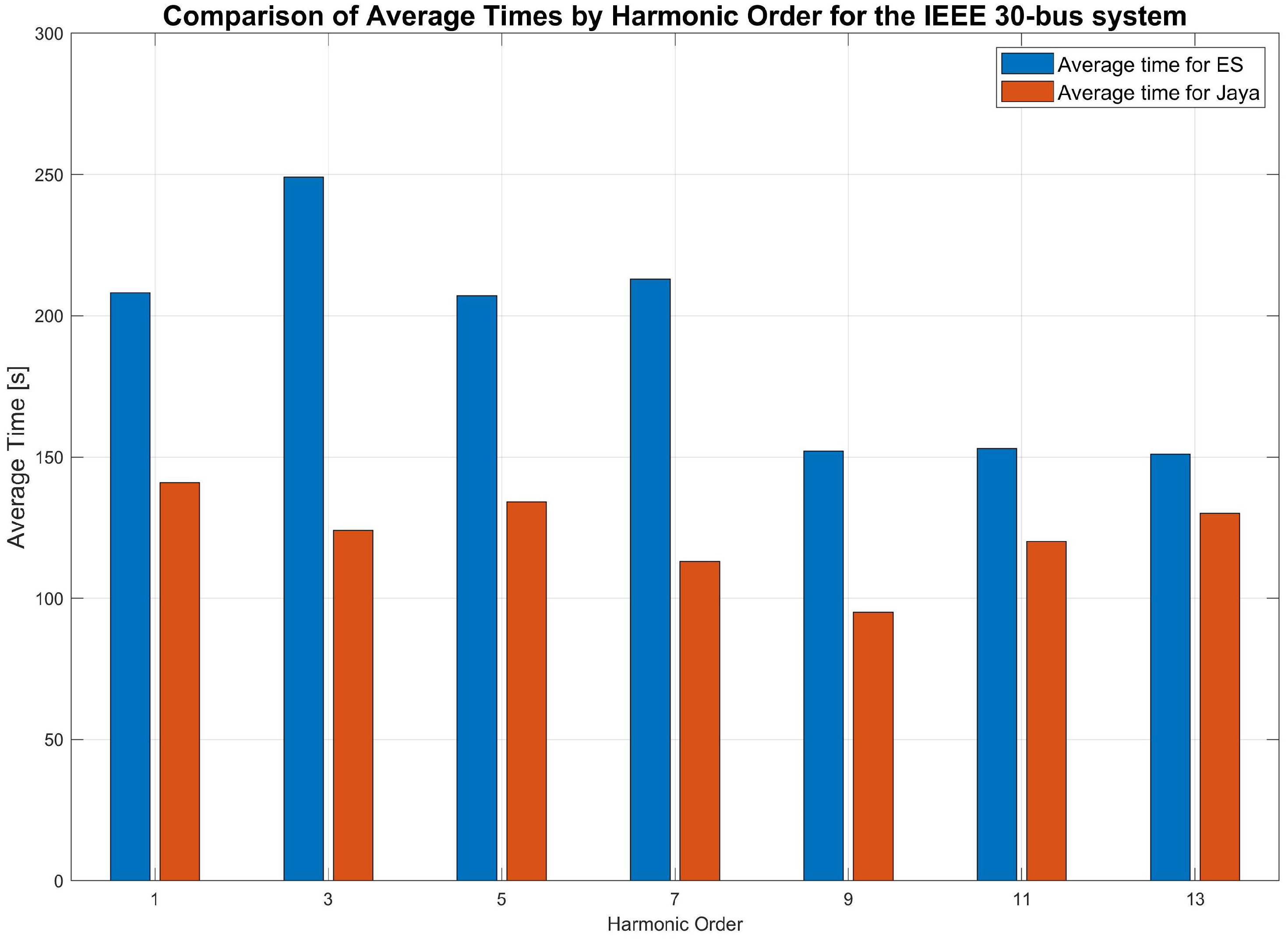
Finally, considering the main characteristic of the Jaya algorithm compared to other methodologies existing in the literature, such as the ES algorithm, which has a simpler code structure and a minimal number of parameters, it is worth addressing the average processing times recorded for both methodologies when applied to the IEEE 14-bus system, shown in Figure 17, as well as when applied to the IEEE 30-bus system, presented in Figure 18. It is observed that in both systems and for all harmonic orders, the Jaya algorithm exhibited considerably lower processing times, finding results of practically the same quality as the ES algorithm in up to 50% less time. This proves that the simplicity of the code and the minimal number of parameters enable a quick solution using the Jaya algorithm.

Figure 17. Comparison between the average times of the Jaya algorithm and the ES algorithm for the IEEE 14-bus system.

Figure 18. Comparison between the average times of the Jaya algorithm and the ES algorithm for the IEEE 30-bus system.

Figure 19 shows the total average time to execute the proposed methodology in this work during the 30 simulations performed. This methodology, which estimates the power flow at the fundamental frequency and all harmonic orders of interest, is applied to both the IEEE 14-bus and IEEE 30-bus systems using the ES and Jaya algorithms, as illustrated in Figure 3. It is observed that with the Jaya algorithm and considering the IEEE 14-bus system, the proposed methodology takes about half the time to obtain the results compared to the ES algorithm. For the IEEE 30-bus system, the Jaya algorithm achieves the desired results in approximately 64% of the total time required by the ES algorithm. Even though the convergence of Jaya may be slower than the ES algorithm, meaning it may take a larger number of generations to converge, Jaya has a lower processing time, which can be attributed to its simplicity and fewer parameters. Thus, corroborating the objective proposed in this work, the Jaya algorithm is significantly faster in achieving equally satisfactory results as the ES algorithm, resulting in lower processing costs as a significant advantage.

Figure 19. Comparison of the average total times between the Jaya algorithm and the ES algorithm for the IEEE 14-bus system and the IEEE 30-bus system.

7. Conclusions

The application of the proposed power flow and HSE methodology based on the Jaya algorithm to the IEEE 14-bus and IEEE 30-bus systems, especially at buses not equipped with PQ meters, using the measured values from other buses, resulted in estimated voltage values with minimal error or little impact on the THD calculation. This led to the determination of more realistic THD values, demonstrating the effectiveness of the proposed methodology based on the Jaya algorithm compared to the results obtained with the ES algorithm.

The adopted strategy for determining the minimum number of meters and selecting the buses to receive these meters proved to be accurate, as the results achieved with both the Jaya and ES algorithms demonstrated the effectiveness of the proposed methodology in estimating the fundamental and harmonic voltages at the other buses from the indicated buses, with minimal absolute errors.

In general, the implementation of the power flow and HSE methodology, based on the Jaya algorithm, proved to be effective in achieving satisfactory results in less time and with lower processing costs compared to those obtained with the ES algorithm. The dynamics of the Jaya algorithm, which aims to move candidate solutions away from the worst solutions and closer to promising solutions, demonstrated robustness in achieving convergence to solutions near to the reference values, allowing for a more precise calculation of THD at the unmonitored buses.

Even though it presented slower convergence compared to the ES algorithm, the absence of parameters and the simplicity of the Jaya algorithm provided a quicker response in the iterative optimization process, without the need for costly empirical parameter adjustments or a suitable set of parameters for each scenario or power system under study, making the proposed methodology applicable to various scenarios with minimal changes in the number of individuals in the initial population and the maximum number of generations.

Based on the obtained results, the presented methodology based on the Jaya algorithm emerges as a promising strategy of HSE, using a minimum number of meters allocated at specific buses through the outlined strategy in this study. This opens avenues for its application in larger, real-world systems, likely yielding equally satisfactory outcomes, through an algorithm that requires few tuning parameters. Such implementation could result in cost savings in studying and identifying harmonic sources in power systems, by reducing the required quantity of PQ meters.

Appendix A.1

Table A1 and Table A2 reproduce the original data of the IEEE 14-bus system, which were used in modeling the system in the electromagnetic transient software PSCAD X4.

Table A1. Line data—IEEE 14-bus system.

Line Number	From Bus	To Bus	Resistance (p.u.)	Reactance (p.u.)	Half Line Charging Susceptance (p.u.)	MVA Rating
1	1	2	0.01938	0.05917	0.02640	120
2	1	5	0.05403	0.22304	0.02190	65
3	2	3	0.04699	0.19797	0.01870	36
4	2	4	0.05811	0.17632	0.02460	65
5	2	5	0.05695	0.17388	0.01700	50
6	3	4	0.06701	0.17103	0.01730	65
7	4	5	0.01335	0.04211	0.00640	45
8	4	7	0	0.20912	0	55
9	4	9	0	0.55618	0	32
10	5	6	0	0.25202	0	45
11	6	11	0.09498	0.1989	0	18
12	6	12	0.12291	0.25581	0	32
13	6	13	0.06615	0.13027	0	32
14	7	8	0	0.17615	0	32
15	7	9	0	0.11001	0	32
16	9	10	0.03181	0.0845	0	32
17	9	14	0.12711	0.27038	0	32
18	10	11	0.08205	0.19207	0	12
19	12	13	0.22092	0.19988	0	12
20	13	14	0.17093	0.34802	0	12

Table A1. Line data—IEEE 14-bus system.

Line Number	From Bus	To Bus	Resistance (p.u.)	Reactance (p.u.)	Half Line Charging Susceptance (p.u.)	MVA Rating
1	1	2	0.01938	0.05917	0.02640	120
2	1	5	0.05403	0.22304	0.02190	65
3	2	3	0.04699	0.19797	0.01870	36
4	2	4	0.05811	0.17632	0.02460	65
5	2	5	0.05695	0.17388	0.01700	50
6	3	4	0.06701	0.17103	0.01730	65
7	4	5	0.01335	0.04211	0.00640	45
8	4	7	0	0.20912	0	55
9	4	9	0	0.55618	0	32
10	5	6	0	0.25202	0	45
11	6	11	0.09498	0.1989	0	18
12	6	12	0.12291	0.25581	0	32
13	6	13	0.06615	0.13027	0	32
14	7	8	0	0.17615	0	32
15	7	9	0	0.11001	0	32
16	9	10	0.03181	0.0845	0	32
17	9	14	0.12711	0.27038	0	32
18	10	11	0.08205	0.19207	0	12
19	12	13	0.22092	0.19988	0	12
20	13	14	0.17093	0.34802	0	12

Table A2. Bus data—IEEE 14 bus system.

Bus Number	Bus Voltage		Generation		Load		Reactive Power Limits
	Magnitude (p.u.)	Phase Angle (Degree)	Real Power (MW)	Reactive Power (MVAR)	Real Power (MW)	Reactive Power (MVAR)	Qmin (MVAR)	Qmax (MVAR))
1	1.060	0	114.17	−16.9	0	0	0	10
2	1.045	0	40.00	0	21.7	12.7	−42.0	50.0
3	1.010	0	0	0	94.2	19.1	23.4	40.0
4	1	0	0	0	47.8	−3.9	–	–
5	1	0	0	0	7.6	1.6	–	–
6	1	0	0	0	11.2	7.5	–	–
7	1	0	0	0	0	0	–	–
8	1	0	0	0	0	0	–	–
9	1	0	0	0	29.5	16.6	–	–
10	1	0	0	0	9.0	5.8	–	–
11	1	0	0	0	3.5	1.8	–	–
12	1	0	0	0	6.1	1.6	–	–
13	1	0	0	0	13.8	5.8	–	–
14	1	0	0	0	14.9	5.0	–	–

Table A2. Bus data—IEEE 14 bus system.

Bus Number	Bus Voltage		Generation		Load		Reactive Power Limits
	Magnitude (p.u.)	Phase Angle (Degree)	Real Power (MW)	Reactive Power (MVAR)	Real Power (MW)	Reactive Power (MVAR)	Qmin (MVAR)	Qmax (MVAR))
1	1.060	0	114.17	−16.9	0	0	0	10
2	1.045	0	40.00	0	21.7	12.7	−42.0	50.0
3	1.010	0	0	0	94.2	19.1	23.4	40.0
4	1	0	0	0	47.8	−3.9	–	–
5	1	0	0	0	7.6	1.6	–	–
6	1	0	0	0	11.2	7.5	–	–
7	1	0	0	0	0	0	–	–
8	1	0	0	0	0	0	–	–
9	1	0	0	0	29.5	16.6	–	–
10	1	0	0	0	9.0	5.8	–	–
11	1	0	0	0	3.5	1.8	–	–
12	1	0	0	0	6.1	1.6	–	–
13	1	0	0	0	13.8	5.8	–	–
14	1	0	0	0	14.9	5.0	–	–

Appendix A.2

Table A3 and Table A4 reproduce the original data of the IEEE 30-bus system, which were used in modeling the system in the electromagnetic transient software PSCAD X4.

Table A3. Line data—IEEE 30-bus system.

Line Number	From Bus	To Bus	Resistance (p.u.)	Reactance (p.u.)	Half Line Charging Susceptance (p.u.)	MVA Rating
1	1	2	0.02	0.06	0.03	130
2	1	3	0.05	0.20	0.02	130
3	2	4	0.06	0.18	0.02	65
4	2	5	0.05	0.02	0	130
5	2	6	0.06	0.18	0.02	65
6	3	4	0.01	0.04	0	130
7	4	6	0.01	0.04	0	90
8	4	12	0	0.23	0	65
9	5	7	0.05	0.12	0.01	70
10	6	7	0.03	0.08	0	130
11	6	8	0.01	0.09	0	32
12	6	9	0	0.21	0	65
13	6	10	0	0.56	0	32
14	6	28	0.07	0.06	0.01	32
15	8	28	0.06	0.20	0.02	32
16	9	11	0	0.21	0	65
17	9	10	0	0.11	0	65
18	10	20	0.09	0.21	0	32
19	10	17	0.03	0.09	0	32
20	10	21	0.03	0.08	0	32
21	10	22	0.07	0.15	0	32
22	12	13	0	0.14	0	65
23	12	14	0.12	0.26	0	32
24	12	15	0.07	0.13	0	32
25	12	16	0.01	0.12	0	32
26	14	15	0.22	0.12	0	16
27	15	18	0.11	0.22	0	16
28	15	23	0.10	0.21	0	16
29	16	17	0.08	0.19	0	16
30	18	19	0.06	0.13	0	16
31	19	20	0.03	0.07	0	32
32	21	22	0.01	0.22	0	32
33	22	24	0.11	0.18	0	16
35	24	25	0.19	0.33	0	16
36	25	26	0.25	0.38	0	16
37	25	27	0.11	0.21	0	16
38	27	29	0.22	0.4	0	16
39	27	30	0.32	0.60	0	16
40	28	27	0	0.4	0	65
41	29	30	0.24	0.45	0	16

Table A3. Line data—IEEE 30-bus system.

Line Number	From Bus	To Bus	Resistance (p.u.)	Reactance (p.u.)	Half Line Charging Susceptance (p.u.)	MVA Rating
1	1	2	0.02	0.06	0.03	130
2	1	3	0.05	0.20	0.02	130
3	2	4	0.06	0.18	0.02	65
4	2	5	0.05	0.02	0	130
5	2	6	0.06	0.18	0.02	65
6	3	4	0.01	0.04	0	130
7	4	6	0.01	0.04	0	90
8	4	12	0	0.23	0	65
9	5	7	0.05	0.12	0.01	70
10	6	7	0.03	0.08	0	130
11	6	8	0.01	0.09	0	32
12	6	9	0	0.21	0	65
13	6	10	0	0.56	0	32
14	6	28	0.07	0.06	0.01	32
15	8	28	0.06	0.20	0.02	32
16	9	11	0	0.21	0	65
17	9	10	0	0.11	0	65
18	10	20	0.09	0.21	0	32
19	10	17	0.03	0.09	0	32
20	10	21	0.03	0.08	0	32
21	10	22	0.07	0.15	0	32
22	12	13	0	0.14	0	65
23	12	14	0.12	0.26	0	32
24	12	15	0.07	0.13	0	32
25	12	16	0.01	0.12	0	32
26	14	15	0.22	0.12	0	16
27	15	18	0.11	0.22	0	16
28	15	23	0.10	0.21	0	16
29	16	17	0.08	0.19	0	16
30	18	19	0.06	0.13	0	16
31	19	20	0.03	0.07	0	32
32	21	22	0.01	0.22	0	32
33	22	24	0.11	0.18	0	16
35	24	25	0.19	0.33	0	16
36	25	26	0.25	0.38	0	16
37	25	27	0.11	0.21	0	16
38	27	29	0.22	0.4	0	16
39	27	30	0.32	0.60	0	16
40	28	27	0	0.4	0	65
41	29	30	0.24	0.45	0	16

Table A4. Bus data—IEEE 30 bus system.

Bus Number	Bus Voltage		Generation		Load		Reactive Power Limits
	Magnitude (p.u.)	Phase Angle (Degree)	Real Power (MW)	Reactive Power (MVAR)	Real Power (MW)	Reactive Power (MVAR)	Qmin (MVAR)	Qmax (MVAR))
1	1	0	0	0	24.963	−4.638	−20	150
2	1	0	21.7	12.7	60.97	27.677	−20	60
3	1	0	2.4	1.2	0	0	0	0
4	1	0	7.6	1.6	0	0	0	0
5	1	0	0	0	0	0	0	0
6	1	0	0	0	0	0	0	0
7	1	0	22.8	10.9	0	0	0	0
8	1	0	30	30	0	0	0	0
9	1	0	0	0	0	0	0	0
10	1	0	5.919	2	0	0	0	0
11	1	0	0	0	0	0	0	0
12	1	0	11.2	7.5	0	0	0	0
13	1	0	0	0	37	13.949	−15	44.7
14	1	0	6.2	1.6	0	0	0	0
15	1	0	8.2	2.5	0	0	0	0
16	1	0	3.5	1.8	0	0	0	0
17	1	0	9	5.8	0	0	0	0
18	1	0	3.2	0.9	0	0	0	0
19	1	0	9.5	3.4	0	0	0	0
20	1	0	2.2	0.7	0	0	0	0
21	1	0	19.669	11.20	0	0	0	0
22	1	0	0	0	31.59	40.34	−15	62.5
23	1	0	3.2	1.6	22.2	8.13	−10	40
24	1	0	15	6.70	0	0	0	0
25	1	0	1.00	0.00	0	0	0	0
26	1	0	3.50	2.30	0	0	0	0
27	1	0	0	0	28.91	10.97	−15	48.7
28	1	0	0	0	0	0	0	0
29	1	0	3.659	0.90	0	0	0	0
30	1	0	12.00	1.90	0	0	0	0

Table A4. Bus data—IEEE 30 bus system.

Bus Number	Bus Voltage		Generation		Load		Reactive Power Limits
	Magnitude (p.u.)	Phase Angle (Degree)	Real Power (MW)	Reactive Power (MVAR)	Real Power (MW)	Reactive Power (MVAR)	Qmin (MVAR)	Qmax (MVAR))
1	1	0	0	0	24.963	−4.638	−20	150
2	1	0	21.7	12.7	60.97	27.677	−20	60
3	1	0	2.4	1.2	0	0	0	0
4	1	0	7.6	1.6	0	0	0	0
5	1	0	0	0	0	0	0	0
6	1	0	0	0	0	0	0	0
7	1	0	22.8	10.9	0	0	0	0
8	1	0	30	30	0	0	0	0
9	1	0	0	0	0	0	0	0
10	1	0	5.919	2	0	0	0	0
11	1	0	0	0	0	0	0	0
12	1	0	11.2	7.5	0	0	0	0
13	1	0	0	0	37	13.949	−15	44.7
14	1	0	6.2	1.6	0	0	0	0
15	1	0	8.2	2.5	0	0	0	0
16	1	0	3.5	1.8	0	0	0	0
17	1	0	9	5.8	0	0	0	0
18	1	0	3.2	0.9	0	0	0	0
19	1	0	9.5	3.4	0	0	0	0
20	1	0	2.2	0.7	0	0	0	0
21	1	0	19.669	11.20	0	0	0	0
22	1	0	0	0	31.59	40.34	−15	62.5
23	1	0	3.2	1.6	22.2	8.13	−10	40
24	1	0	15	6.70	0	0	0	0
25	1	0	1.00	0.00	0	0	0	0
26	1	0	3.50	2.30	0	0	0	0
27	1	0	0	0	28.91	10.97	−15	48.7
28	1	0	0	0	0	0	0	0
29	1	0	3.659	0.90	0	0	0	0
30	1	0	12.00	1.90	0	0	0	0

Appendix B.1

Table A5, Table A6, Table A7, Table A8, Table A9 and Table A10 present the fundamental and harmonic component values of current and voltage derived from the power flow and harmonic state analysis for the IEEE 14-bus system using the electromagnetic transient software PSCAD X4. These values are based on the current injection harmonics in randomly selected buses.

Table A5. Reference values of magnitude in p.u. and phase in degrees for the fundamental current and the 3rd- and 5th-order current harmonics for the IEEE 14-bus system.

Bus	I1h		I3h		I5h
	Magnitude	Phase	Magnitude	Phase	Magnitude	Phase
1	1.3568	0.8469	0.0675	114.0084	0.0104	1.7873
2	1.0610	25.7289	0.0769	52.3577	0.0135	1.7903
3	0.3546	−77.9438	0.0303	124.6684	0.0038	14.0743
4	3.0349	114.7311	0.1398	131.0776	0.0539	−5.4048
5	2.3628	−113.9661	0.2465	−71.8184	0.0822	178.0589
6	1.0942	−154.4807	0.0707	−69.5813	0.0203	179.2846
7	1.1543	−161.3394	0.0645	−96.9026	0.0129	161.8508
8	0.4530	−2.6687	0.0240	77.4207	0.0040	−15.1816
9	1.2540	12.0537	0.0618	74.9923	0.0115	−16.0899
10	1.3448	−165.2971	0.0381	−99.6608	0.0077	167.0406
11	1.5534	10.3182	0.0320	110.8868	0.0068	−0.0682
12	0.1384	23.2814	0.0239	102.9830	0.0126	−1.8550
13	0.2785	30.9553	0.0490	113.0734	0.0102	−1.9336
14	0.2758	−176.6854	0.0150	−59.1108	0.0015	165.4553

Table A5. Reference values of magnitude in p.u. and phase in degrees for the fundamental current and the 3rd- and 5th-order current harmonics for the IEEE 14-bus system.

Bus	I1h		I3h		I5h
	Magnitude	Phase	Magnitude	Phase	Magnitude	Phase
1	1.3568	0.8469	0.0675	114.0084	0.0104	1.7873
2	1.0610	25.7289	0.0769	52.3577	0.0135	1.7903
3	0.3546	−77.9438	0.0303	124.6684	0.0038	14.0743
4	3.0349	114.7311	0.1398	131.0776	0.0539	−5.4048
5	2.3628	−113.9661	0.2465	−71.8184	0.0822	178.0589
6	1.0942	−154.4807	0.0707	−69.5813	0.0203	179.2846
7	1.1543	−161.3394	0.0645	−96.9026	0.0129	161.8508
8	0.4530	−2.6687	0.0240	77.4207	0.0040	−15.1816
9	1.2540	12.0537	0.0618	74.9923	0.0115	−16.0899
10	1.3448	−165.2971	0.0381	−99.6608	0.0077	167.0406
11	1.5534	10.3182	0.0320	110.8868	0.0068	−0.0682
12	0.1384	23.2814	0.0239	102.9830	0.0126	−1.8550
13	0.2785	30.9553	0.0490	113.0734	0.0102	−1.9336
14	0.2758	−176.6854	0.0150	−59.1108	0.0015	165.4553

Table A6. Reference values of magnitude in p.u. and phase in degrees for the fundamental voltage and the 3rd- and 5th-order voltage harmonics for the IEEE 14-bus system.

Bus	V1h		V3h		V5h
	Magnitude	Phase	Magnitude	Phase	Magnitude	Phase
1	1.0389	0.0000	0.0196	49.7381	0.0007	54.5349
2	1.0249	−2.2324	0.0241	51.6591	0.0009	54.6651
3	1.0474	−5.6707	0.0181	33.0986	0.0022	84.7141
4	0.9918	−9.3622	0.0286	23.3699	0.0011	2.5361
5	1.0733	−8.4336	0.0475	27.2249	0.0116	−79.7017
6	1.0475	−8.4312	0.0372	27.2248	0.0046	−79.0903
7	1.0357	−9.4191	0.0356	24.6004	0.0029	−84.2933
8	1.0139	−5.1264	0.0248	37.4928	0.0009	51.8321
9	1.0079	−6.5582	0.0273	33.5427	0.0007	35.1230
10	1.0297	−9.0500	0.0322	24.2313	0.0020	−84.0741
11	1.0341	0.4852	0.0252	26.6973	0.0002	21.3587
12	1.0334	−6.7345	0.0204	35.3104	0.0071	87.7918
13	1.0277	−7.0353	0.0211	32.2701	0.0034	86.1968
14	1.0142	−9.3867	0.0315	33.0450	0.0006	68.3699

Table A6. Reference values of magnitude in p.u. and phase in degrees for the fundamental voltage and the 3rd- and 5th-order voltage harmonics for the IEEE 14-bus system.

Bus	V1h		V3h		V5h
	Magnitude	Phase	Magnitude	Phase	Magnitude	Phase
1	1.0389	0.0000	0.0196	49.7381	0.0007	54.5349
2	1.0249	−2.2324	0.0241	51.6591	0.0009	54.6651
3	1.0474	−5.6707	0.0181	33.0986	0.0022	84.7141
4	0.9918	−9.3622	0.0286	23.3699	0.0011	2.5361
5	1.0733	−8.4336	0.0475	27.2249	0.0116	−79.7017
6	1.0475	−8.4312	0.0372	27.2248	0.0046	−79.0903
7	1.0357	−9.4191	0.0356	24.6004	0.0029	−84.2933
8	1.0139	−5.1264	0.0248	37.4928	0.0009	51.8321
9	1.0079	−6.5582	0.0273	33.5427	0.0007	35.1230
10	1.0297	−9.0500	0.0322	24.2313	0.0020	−84.0741
11	1.0341	0.4852	0.0252	26.6973	0.0002	21.3587
12	1.0334	−6.7345	0.0204	35.3104	0.0071	87.7918
13	1.0277	−7.0353	0.0211	32.2701	0.0034	86.1968
14	1.0142	−9.3867	0.0315	33.0450	0.0006	68.3699

Table A7. Reference values of magnitude in p.u. and phase in degrees for the 7th- and 9th-order current harmonics for the IEEE 14-bus system.

Bus	I7h		I9h
	Magnitude	Phase	Magnitude	Phase
1	0.0042	−73.3047	0.0014	−159.6064
2	0.0046	−97.2743	0.0038	−40.3494
3	0.0069	−22.2887	0.0040	−2.4660
4	0.0164	−128.3670	0.0235	177.1767
5	0.0318	89.5932	0.0178	26.5938
6	0.0119	170.7023	0.0157	171.3318
7	0.0115	−73.6166	0.0187	165.3096
8	0.0028	97.4352	0.0067	−17.4348
9	0.0116	108.4548	0.0241	−18.7536
10	0.0060	−79.7852	0.0135	163.6955
11	0.0025	−26.8629	0.0033	−13.1680
12	0.0087	−9.3997	0.0103	−7.8251
13	0.0039	−35.3470	0.0050	−21.7709
14	0.0023	−70.9486	0.0034	161.6506

Table A7. Reference values of magnitude in p.u. and phase in degrees for the 7th- and 9th-order current harmonics for the IEEE 14-bus system.

Bus	I7h		I9h
	Magnitude	Phase	Magnitude	Phase
1	0.0042	−73.3047	0.0014	−159.6064
2	0.0046	−97.2743	0.0038	−40.3494
3	0.0069	−22.2887	0.0040	−2.4660
4	0.0164	−128.3670	0.0235	177.1767
5	0.0318	89.5932	0.0178	26.5938
6	0.0119	170.7023	0.0157	171.3318
7	0.0115	−73.6166	0.0187	165.3096
8	0.0028	97.4352	0.0067	−17.4348
9	0.0116	108.4548	0.0241	−18.7536
10	0.0060	−79.7852	0.0135	163.6955
11	0.0025	−26.8629	0.0033	−13.1680
12	0.0087	−9.3997	0.0103	−7.8251
13	0.0039	−35.3470	0.0050	−21.7709
14	0.0023	−70.9486	0.0034	161.6506

Table A8. Reference values of magnitude in p.u. and phase in degrees for the 7th- and 9th-order voltage harmonics for the IEEE 14-bus system.

Bus	V7h		V9h
	Magnitude	Phase	Magnitude	Phase
1	0.0010	4.1341	0.0042	54.3987
2	0.0010	−5.0945	0.0044	55.7077
3	0.0044	61.2362	0.0045	66.6699
4	0.0020	−80.6971	0.0039	−78.4343
5	0.0060	−158.3638	0.0024	123.9482
6	0.0011	18.0356	0.0023	−57.4554
7	0.0052	20.7174	0.0072	−75.0046
8	0.0017	24.7758	0.0047	50.1152
9	0.0016	17.5193	0.0042	47.1212
10	0.0048	24.0006	0.0053	−72.8899
11	0.0044	40.0947	0.0017	−20.4970
12	0.0105	76.2687	0.0131	81.7285
13	0.0063	63.6326	0.0063	70.9736
14	0.0058	41.7860	0.0017	−10.1490

Table A8. Reference values of magnitude in p.u. and phase in degrees for the 7th- and 9th-order voltage harmonics for the IEEE 14-bus system.

Bus	V7h		V9h
	Magnitude	Phase	Magnitude	Phase
1	0.0010	4.1341	0.0042	54.3987
2	0.0010	−5.0945	0.0044	55.7077
3	0.0044	61.2362	0.0045	66.6699
4	0.0020	−80.6971	0.0039	−78.4343
5	0.0060	−158.3638	0.0024	123.9482
6	0.0011	18.0356	0.0023	−57.4554
7	0.0052	20.7174	0.0072	−75.0046
8	0.0017	24.7758	0.0047	50.1152
9	0.0016	17.5193	0.0042	47.1212
10	0.0048	24.0006	0.0053	−72.8899
11	0.0044	40.0947	0.0017	−20.4970
12	0.0105	76.2687	0.0131	81.7285
13	0.0063	63.6326	0.0063	70.9736
14	0.0058	41.7860	0.0017	−10.1490

Table A9. Reference values of magnitude in p.u. and phase in degrees for the 11th- and 13th-order current harmonics for the IEEE 14-bus system.

Bus	I11h		I13h
	Magnitude	Phase	Magnitude	Phase
1	0.0000	45.0055	0.0040	−26.2923
2	0.0003	−109.0205	0.0048	147.8820
3	0.0004	−5.2698	0.0011	2.9953
4	0.0019	128.7342	0.0041	53.8713
5	0.0010	16.3347	0.0017	32.1031
6	0.0014	158.9590	0.0013	158.3837
7	0.0020	134.7139	0.0027	68.3087
8	0.0007	−51.7150	0.0013	−125.0988
9	0.0025	−57.0338	0.0045	−115.7826
10	0.0015	132.5732	0.0021	74.3176
11	0.0003	−30.3041	0.0002	−61.6939
12	0.0007	−18.9440	0.0007	−18.7090
13	0.0005	−42.8747	0.0004	−79.9085
14	0.0004	21.1937	0.0010	21.3771

Table A9. Reference values of magnitude in p.u. and phase in degrees for the 11th- and 13th-order current harmonics for the IEEE 14-bus system.

Bus	I11h		I13h
	Magnitude	Phase	Magnitude	Phase
1	0.0000	45.0055	0.0040	−26.2923
2	0.0003	−109.0205	0.0048	147.8820
3	0.0004	−5.2698	0.0011	2.9953
4	0.0019	128.7342	0.0041	53.8713
5	0.0010	16.3347	0.0017	32.1031
6	0.0014	158.9590	0.0013	158.3837
7	0.0020	134.7139	0.0027	68.3087
8	0.0007	−51.7150	0.0013	−125.0988
9	0.0025	−57.0338	0.0045	−115.7826
10	0.0015	132.5732	0.0021	74.3176
11	0.0003	−30.3041	0.0002	−61.6939
12	0.0007	−18.9440	0.0007	−18.7090
13	0.0005	−42.8747	0.0004	−79.9085
14	0.0004	21.1937	0.0010	21.3771

Table A10. Reference values of magnitude in p.u. and phase in degrees for the 11th- and 13th-order voltage harmonics for the IEEE 14-bus system.

Bus	V11h		V13h
	Magnitude	Phase	Magnitude	Phase
1	0.0008	14.7025	0.0042	0.0000
2	0.0008	11.7325	0.0038	−51.7604
3	0.0006	51.4235	0.0007	7.6872
4	0.0004	−123.8458	0.0009	166.9942
5	0.0001	124.2232	0.0001	131.4582
6	0.0002	−64.7378	0.0004	−45.8265
7	0.0007	−99.8268	0.0005	−140.0438
8	0.0009	24.7520	0.0029	−33.3961
9	0.0008	28.7982	0.0020	−16.5888
10	0.0005	−97.9958	0.0003	−132.1348
11	0.0001	−15.9827	0.0003	−18.9810
12	0.0013	69.7222	0.0015	61.6654
13	0.0009	62.0050	0.0010	44.9332
14	0.0012	79.7056	0.0018	78.7671

Table A10. Reference values of magnitude in p.u. and phase in degrees for the 11th- and 13th-order voltage harmonics for the IEEE 14-bus system.

Bus	V11h		V13h
	Magnitude	Phase	Magnitude	Phase
1	0.0008	14.7025	0.0042	0.0000
2	0.0008	11.7325	0.0038	−51.7604
3	0.0006	51.4235	0.0007	7.6872
4	0.0004	−123.8458	0.0009	166.9942
5	0.0001	124.2232	0.0001	131.4582
6	0.0002	−64.7378	0.0004	−45.8265
7	0.0007	−99.8268	0.0005	−140.0438
8	0.0009	24.7520	0.0029	−33.3961
9	0.0008	28.7982	0.0020	−16.5888
10	0.0005	−97.9958	0.0003	−132.1348
11	0.0001	−15.9827	0.0003	−18.9810
12	0.0013	69.7222	0.0015	61.6654
13	0.0009	62.0050	0.0010	44.9332
14	0.0012	79.7056	0.0018	78.7671

Appendix B.2

Table A11, Table A12, Table A13, Table A14, Table A15 and Table A16 present the fundamental and harmonic component values of current and voltage derived from the power flow and harmonic state analysis for the IEEE 30-bus system using the electromagnetic transient software PSCAD. These values are based on the current injection harmonics in randomly selected buses.

Table A11. Reference values of magnitude in p.u. and phase in degrees for the fundamental current and the 3rd- and 5th-order current harmonics for the IEEE 30-bus system.

Bus	I1h		I3h		I5h
	Magnitude	Phase	Magnitude	Phase	Magnitude	Phase
1	2.4225	4.6303	0.0297	101.7929	0.0277	106.5383
2	0.3117	−71.0712	0.0334	101.6414	0.0339	105.7678
3	0.0429	114.5359	0.0212	−56.6931	0.0201	−19.8704
4	0.0914	134.8175	0.0210	−56.9781	0.0191	−19.7931
5	0.6599	176.9164	0.0077	94.6504	0.0073	90.4240
6	1.3085	−4.0181	0.0446	−86.3126	0.0646	−63.5168
7	1.5177	166.8849	0.0559	97.5524	0.0555	99.1196
8	0.4855	178.1453	0.0408	93.2719	0.0489	94.4718
9	0.0100	78.0838	0.0007	170.1796	0.0000	63.3482
10	0.2440	−91.0078	0.0199	−87.6524	0.0680	−104.0201
11	0.1528	−109.5362	0.0077	96.0748	0.0092	87.9318
12	0.1329	128.1885	0.0257	−66.1200	0.0016	−61.6546
13	0.1036	−111.2879	0.0129	105.8729	0.0087	99.0378
14	0.0612	150.4783	0.0048	−88.1826	0.0030	−44.4672
15	0.0819	147.9532	0.0100	−74.6288	0.0022	−52.2500
16	0.0658	144.6928	0.0161	−64.1485	0.0146	23.7366
17	0.1221	131.5175	0.0176	135.1811	0.0238	−152.6003
18	0.0320	148.8493	0.0013	177.8790	0.0017	164.9190
19	0.0973	144.7158	0.0046	−100.5731	0.0010	−80.6940
20	0.0265	−40.6767	0.0037	−33.6055	0.0076	50.4356
21	0.1989	131.9794	0.0049	−132.8660	0.0055	151.1641
22	0.1321	134.5346	0.0041	−109.9021	0.0043	130.7205
23	0.0344	137.9697	0.0106	−63.9712	0.0040	−29.9911
24	0.0864	150.3353	0.0053	−133.6797	0.0140	−134.4625
25	0.0002	−105.9906	0.0000	−98.6402	0.0000	−119.1604
26	0.0415	130.9871	0.0011	161.9104	0.0017	145.4195
27	0.0101	77.1564	0.0004	173.3416	0.0000	77.4757
28	0.0387	78.5974	0.0016	74.3719	0.0037	86.3870
29	0.0254	143.6333	0.0006	163.8730	0.0009	146.9362
30	0.1080	152.9805	0.0025	164.3274	0.0040	143.5933

Table A11. Reference values of magnitude in p.u. and phase in degrees for the fundamental current and the 3rd- and 5th-order current harmonics for the IEEE 30-bus system.

Bus	I1h		I3h		I5h
	Magnitude	Phase	Magnitude	Phase	Magnitude	Phase
1	2.4225	4.6303	0.0297	101.7929	0.0277	106.5383
2	0.3117	−71.0712	0.0334	101.6414	0.0339	105.7678
3	0.0429	114.5359	0.0212	−56.6931	0.0201	−19.8704
4	0.0914	134.8175	0.0210	−56.9781	0.0191	−19.7931
5	0.6599	176.9164	0.0077	94.6504	0.0073	90.4240
6	1.3085	−4.0181	0.0446	−86.3126	0.0646	−63.5168
7	1.5177	166.8849	0.0559	97.5524	0.0555	99.1196
8	0.4855	178.1453	0.0408	93.2719	0.0489	94.4718
9	0.0100	78.0838	0.0007	170.1796	0.0000	63.3482
10	0.2440	−91.0078	0.0199	−87.6524	0.0680	−104.0201
11	0.1528	−109.5362	0.0077	96.0748	0.0092	87.9318
12	0.1329	128.1885	0.0257	−66.1200	0.0016	−61.6546
13	0.1036	−111.2879	0.0129	105.8729	0.0087	99.0378
14	0.0612	150.4783	0.0048	−88.1826	0.0030	−44.4672
15	0.0819	147.9532	0.0100	−74.6288	0.0022	−52.2500
16	0.0658	144.6928	0.0161	−64.1485	0.0146	23.7366
17	0.1221	131.5175	0.0176	135.1811	0.0238	−152.6003
18	0.0320	148.8493	0.0013	177.8790	0.0017	164.9190
19	0.0973	144.7158	0.0046	−100.5731	0.0010	−80.6940
20	0.0265	−40.6767	0.0037	−33.6055	0.0076	50.4356
21	0.1989	131.9794	0.0049	−132.8660	0.0055	151.1641
22	0.1321	134.5346	0.0041	−109.9021	0.0043	130.7205
23	0.0344	137.9697	0.0106	−63.9712	0.0040	−29.9911
24	0.0864	150.3353	0.0053	−133.6797	0.0140	−134.4625
25	0.0002	−105.9906	0.0000	−98.6402	0.0000	−119.1604
26	0.0415	130.9871	0.0011	161.9104	0.0017	145.4195
27	0.0101	77.1564	0.0004	173.3416	0.0000	77.4757
28	0.0387	78.5974	0.0016	74.3719	0.0037	86.3870
29	0.0254	143.6333	0.0006	163.8730	0.0009	146.9362
30	0.1080	152.9805	0.0025	164.3274	0.0040	143.5933

Table A12. Reference values of magnitude in p.u. and phase in degrees for the fundamental voltage and the 3rd- and 5th-order voltage harmonics for the IEEE 30-bus system.

Bus	V1h		V3h		V5h
	Magnitude	Phase	Magnitude	Phase	Magnitude	Phase
1	1.0601	0.0000	0.0052	0.0000	0.0073	0.0000
2	1.0427	−5.3512	0.0057	−1.2333	0.0084	−2.6467
3	1.0212	−7.0593	0.0178	6.7374	0.0246	15.4302
4	1.0121	−8.6974	0.0181	4.4400	0.0252	9.7507
5	1.0084	−15.2166	0.0013	−14.7333	0.0018	−28.2391
6	1.0110	−10.2207	0.0150	−0.4475	0.0241	2.2046
7	0.9878	−16.5200	0.0012	−18.7118	0.0019	−36.3926
8	1.0098	−11.3616	0.0109	−0.1609	0.0163	1.3840
9	1.0503	−13.3801	0.0268	−3.7503	0.0496	−16.3213
10	1.0447	−14.9323	0.0354	−3.4405	0.0684	−18.7517
11	1.0819	−13.5606	0.0221	−5.8640	0.0404	−19.6643
12	1.0550	−14.4237	0.0412	4.8373	0.0441	−6.1853
13	1.0694	−14.5165	0.0359	3.1853	0.0383	−8.5845
14	1.0406	−15.2693	0.0448	3.2748	0.0489	−6.3038
15	1.0366	−15.3201	0.0447	2.8281	0.0503	−9.1232
16	1.0406	−15.0896	0.0424	2.4962	0.0519	−8.8895
17	1.0373	−15.2310	0.0352	−4.7272	0.0679	−20.7700
18	1.0304	−15.7252	0.0431	0.3966	0.0544	−12.7432
19	1.0297	−15.7745	0.0423	−0.4353	0.0570	−13.5611
20	1.0347	−15.5163	0.0410	−0.4460	0.0580	−14.0665
21	1.0275	−15.5646	0.0369	−4.6523	0.0668	−20.8442
22	1.0264	−15.6108	0.0371	−4.6255	0.0665	−20.9705
23	1.0246	−15.7266	0.0457	1.3109	0.0566	−13.1335
24	1.0169	−15.9275	0.0387	−4.4781	0.0638	−21.8784
25	1.0132	−15.4230	0.0299	−6.6277	0.0482	−23.5341
26	0.9957	−15.8426	0.0294	−8.8384	0.0473	−27.2579
27	1.0193	−14.8502	0.0247	−7.4929	0.0389	−22.8831
28	1.0064	−10.9248	0.0152	−1.8767	0.0242	−2.4239
29	0.9996	−16.0812	0.0241	−11.5798	0.0376	−29.8528
30	0.9882	−16.9639	0.0239	−14.3649	0.0370	−34.6621

Table A12. Reference values of magnitude in p.u. and phase in degrees for the fundamental voltage and the 3rd- and 5th-order voltage harmonics for the IEEE 30-bus system.

Bus	V1h		V3h		V5h
	Magnitude	Phase	Magnitude	Phase	Magnitude	Phase
1	1.0601	0.0000	0.0052	0.0000	0.0073	0.0000
2	1.0427	−5.3512	0.0057	−1.2333	0.0084	−2.6467
3	1.0212	−7.0593	0.0178	6.7374	0.0246	15.4302
4	1.0121	−8.6974	0.0181	4.4400	0.0252	9.7507
5	1.0084	−15.2166	0.0013	−14.7333	0.0018	−28.2391
6	1.0110	−10.2207	0.0150	−0.4475	0.0241	2.2046
7	0.9878	−16.5200	0.0012	−18.7118	0.0019	−36.3926
8	1.0098	−11.3616	0.0109	−0.1609	0.0163	1.3840
9	1.0503	−13.3801	0.0268	−3.7503	0.0496	−16.3213
10	1.0447	−14.9323	0.0354	−3.4405	0.0684	−18.7517
11	1.0819	−13.5606	0.0221	−5.8640	0.0404	−19.6643
12	1.0550	−14.4237	0.0412	4.8373	0.0441	−6.1853
13	1.0694	−14.5165	0.0359	3.1853	0.0383	−8.5845
14	1.0406	−15.2693	0.0448	3.2748	0.0489	−6.3038
15	1.0366	−15.3201	0.0447	2.8281	0.0503	−9.1232
16	1.0406	−15.0896	0.0424	2.4962	0.0519	−8.8895
17	1.0373	−15.2310	0.0352	−4.7272	0.0679	−20.7700
18	1.0304	−15.7252	0.0431	0.3966	0.0544	−12.7432
19	1.0297	−15.7745	0.0423	−0.4353	0.0570	−13.5611
20	1.0347	−15.5163	0.0410	−0.4460	0.0580	−14.0665
21	1.0275	−15.5646	0.0369	−4.6523	0.0668	−20.8442
22	1.0264	−15.6108	0.0371	−4.6255	0.0665	−20.9705
23	1.0246	−15.7266	0.0457	1.3109	0.0566	−13.1335
24	1.0169	−15.9275	0.0387	−4.4781	0.0638	−21.8784
25	1.0132	−15.4230	0.0299	−6.6277	0.0482	−23.5341
26	0.9957	−15.8426	0.0294	−8.8384	0.0473	−27.2579
27	1.0193	−14.8502	0.0247	−7.4929	0.0389	−22.8831
28	1.0064	−10.9248	0.0152	−1.8767	0.0242	−2.4239
29	0.9996	−16.0812	0.0241	−11.5798	0.0376	−29.8528
30	0.9882	−16.9639	0.0239	−14.3649	0.0370	−34.6621

Table A13. Reference values of magnitude in p.u. and phase in degrees for the 7th- and 9th-order current harmonics for the IEEE 30-bus system.

Bus	I7h		I9h
	Magnitude	Phase	Magnitude	Phase
1	0.0141	110.4383	0.0413	113.4899
2	0.0163	104.2281	0.0483	112.3841
3	0.0196	−26.8088	0.0306	−40.0922
4	0.0196	−27.2285	0.0311	−43.7682
5	0.0033	81.1779	0.0091	81.5128
6	0.0330	−53.7070	0.0733	−51.3579
7	0.0194	87.8418	0.0444	114.8477
8	0.0151	59.0112	0.0504	122.2711
9	0.0000	−113.3607	0.0000	164.5245
10	0.0822	−177.0948	0.0943	135.7174
11	0.0052	24.2534	0.0029	−10.7531
12	0.0040	−28.4571	0.0097	−64.0422
13	0.0025	76.9512	0.0045	125.7667
14	0.0046	−31.6495	0.0104	−57.5931
15	0.0043	−25.6593	0.0021	−176.6715
16	0.0273	−19.5503	0.0385	−56.4748
17	0.0347	154.7966	0.0462	116.7126
18	0.0008	113.2980	0.0004	148.0787
19	0.0041	−6.4142	0.0012	102.6376
20	0.0107	−12.7264	0.0175	−53.5896
21	0.0083	46.6772	0.0083	38.7982
22	0.0069	26.1570	0.0080	−29.1297
23	0.0051	−25.6802	0.0110	−47.8208
24	0.0144	162.7108	0.0113	132.1101
25	0.0000	172.2081	0.0000	155.8399
26	0.0011	79.5354	0.0005	66.4725
27	0.0000	144.8736	0.0000	147.7954
28	0.0023	65.0375	0.0076	102.7021
29	0.0005	82.9238	0.0002	118.4700
30	0.0022	76.4090	0.0010	109.8880

Table A13. Reference values of magnitude in p.u. and phase in degrees for the 7th- and 9th-order current harmonics for the IEEE 30-bus system.

Bus	I7h		I9h
	Magnitude	Phase	Magnitude	Phase
1	0.0141	110.4383	0.0413	113.4899
2	0.0163	104.2281	0.0483	112.3841
3	0.0196	−26.8088	0.0306	−40.0922
4	0.0196	−27.2285	0.0311	−43.7682
5	0.0033	81.1779	0.0091	81.5128
6	0.0330	−53.7070	0.0733	−51.3579
7	0.0194	87.8418	0.0444	114.8477
8	0.0151	59.0112	0.0504	122.2711
9	0.0000	−113.3607	0.0000	164.5245
10	0.0822	−177.0948	0.0943	135.7174
11	0.0052	24.2534	0.0029	−10.7531
12	0.0040	−28.4571	0.0097	−64.0422
13	0.0025	76.9512	0.0045	125.7667
14	0.0046	−31.6495	0.0104	−57.5931
15	0.0043	−25.6593	0.0021	−176.6715
16	0.0273	−19.5503	0.0385	−56.4748
17	0.0347	154.7966	0.0462	116.7126
18	0.0008	113.2980	0.0004	148.0787
19	0.0041	−6.4142	0.0012	102.6376
20	0.0107	−12.7264	0.0175	−53.5896
21	0.0083	46.6772	0.0083	38.7982
22	0.0069	26.1570	0.0080	−29.1297
23	0.0051	−25.6802	0.0110	−47.8208
24	0.0144	162.7108	0.0113	132.1101
25	0.0000	172.2081	0.0000	155.8399
26	0.0011	79.5354	0.0005	66.4725
27	0.0000	144.8736	0.0000	147.7954
28	0.0023	65.0375	0.0076	102.7021
29	0.0005	82.9238	0.0002	118.4700
30	0.0022	76.4090	0.0010	109.8880

Table A14. Reference values of magnitude in p.u. and phase in degrees for the 7th- and 9th-order voltage harmonics for the IEEE 30-bus system.

Bus	V7h		V9h
	Magnitude	Phase	Magnitude	Phase
1	0.0049	0.0000	0.0172	0.0000
2	0.0051	−7.8935	0.0171	−1.6754
3	0.0179	23.8568	0.0586	25.0809
4	0.0153	14.1517	0.0501	22.6895
5	0.0011	−44.6149	0.0034	−48.9590
6	0.0117	−9.6284	0.0323	15.8900
7	0.0012	−57.0078	0.0042	−67.0073
8	0.0091	−2.0414	0.0200	0.7528
9	0.0382	−84.4256	0.0264	−123.5510
10	0.0607	−89.0056	0.0573	−133.8570
11	0.0310	−88.9332	0.0215	−129.2516
12	0.0172	−33.0342	0.0376	11.3306
13	0.0149	−36.2715	0.0325	7.2377
14	0.0187	−29.9011	0.0427	12.1779
15	0.0196	−46.9106	0.0288	3.9094
16	0.0220	−54.0563	0.0257	4.7365
17	0.0603	−91.8058	0.0568	−137.5212
18	0.0250	−65.4657	0.0150	−29.4747
19	0.0290	−71.3968	0.0132	−71.8265
20	0.0330	−75.4317	0.0151	−89.6589
21	0.0547	−91.8177	0.0490	−137.2982
22	0.0539	−91.7808	0.0466	−136.4792
23	0.0264	−69.4514	0.0182	−5.8386
24	0.0471	−91.2477	0.0292	−125.2941
25	0.0310	−90.7513	0.0143	−100.3610
26	0.0304	−96.0223	0.0139	−106.9738
27	0.0212	−86.0616	0.0109	−48.0127
28	0.0111	−20.0752	0.0293	11.1500
29	0.0203	−95.6808	0.0103	−59.6021
30	0.0199	−102.3893	0.0100	−67.8574

Table A14. Reference values of magnitude in p.u. and phase in degrees for the 7th- and 9th-order voltage harmonics for the IEEE 30-bus system.

Bus	V7h		V9h
	Magnitude	Phase	Magnitude	Phase
1	0.0049	0.0000	0.0172	0.0000
2	0.0051	−7.8935	0.0171	−1.6754
3	0.0179	23.8568	0.0586	25.0809
4	0.0153	14.1517	0.0501	22.6895
5	0.0011	−44.6149	0.0034	−48.9590
6	0.0117	−9.6284	0.0323	15.8900
7	0.0012	−57.0078	0.0042	−67.0073
8	0.0091	−2.0414	0.0200	0.7528
9	0.0382	−84.4256	0.0264	−123.5510
10	0.0607	−89.0056	0.0573	−133.8570
11	0.0310	−88.9332	0.0215	−129.2516
12	0.0172	−33.0342	0.0376	11.3306
13	0.0149	−36.2715	0.0325	7.2377
14	0.0187	−29.9011	0.0427	12.1779
15	0.0196	−46.9106	0.0288	3.9094
16	0.0220	−54.0563	0.0257	4.7365
17	0.0603	−91.8058	0.0568	−137.5212
18	0.0250	−65.4657	0.0150	−29.4747
19	0.0290	−71.3968	0.0132	−71.8265
20	0.0330	−75.4317	0.0151	−89.6589
21	0.0547	−91.8177	0.0490	−137.2982
22	0.0539	−91.7808	0.0466	−136.4792
23	0.0264	−69.4514	0.0182	−5.8386
24	0.0471	−91.2477	0.0292	−125.2941
25	0.0310	−90.7513	0.0143	−100.3610
26	0.0304	−96.0223	0.0139	−106.9738
27	0.0212	−86.0616	0.0109	−48.0127
28	0.0111	−20.0752	0.0293	11.1500
29	0.0203	−95.6808	0.0103	−59.6021
30	0.0199	−102.3893	0.0100	−67.8574

Table A15. Reference values of magnitude in p.u. and phase in degrees for the 11th- and 13th-order current harmonics for the IEEE 30-bus system.

Bus	I11h		I13h
	Magnitude	Phase	Magnitude	Phase
1	0.0883	115.1230	0.0595	115.7186
2	0.1114	113.5960	0.0834	116.7914
3	0.0331	−6.5337	0.0285	137.1271
4	0.0321	−13.7671	0.0464	30.2879
5	0.0189	74.5816	0.0120	69.5983
6	0.1135	−38.5479	0.0226	−39.0112
7	0.0938	121.9464	0.0649	129.4856
8	0.1124	130.8532	0.0589	128.4795
9	0.0001	159.3623	0.0000	163.4049
10	0.1464	123.5815	0.1146	112.9497
11	0.0012	−7.1167	0.0003	−69.6160
12	0.0078	−163.2642	0.0118	−15.3862
13	0.0080	137.9449	0.0067	163.2837
14	0.0147	−48.3204	0.0137	−8.9153
15	0.0143	−48.5322	0.0054	−145.3856
16	0.0508	−56.6206	0.0239	−61.6100
17	0.0581	114.2234	0.0332	118.2853
18	0.0013	−167.7596	0.0014	−143.2664
19	0.0023	−178.1561	0.0037	−21.8539
20	0.0220	−54.1045	0.0102	−54.8897
21	0.0205	−16.0848	0.0177	12.2930
22	0.0178	−57.9862	0.0227	−86.0469
23	0.0013	−178.5032	0.0148	3.1012
24	0.0131	−162.7641	0.0601	−124.0382
25	0.0000	−116.8635	0.0002	−117.5470
26	0.0011	141.6739	0.0027	144.2810
27	0.0000	−155.1066	0.0001	−124.5232
28	0.0249	110.8053	0.0257	117.4348
29	0.0009	155.7638	0.0014	148.0514
30	0.0041	144.4010	0.0061	134.3415

Table A15. Reference values of magnitude in p.u. and phase in degrees for the 11th- and 13th-order current harmonics for the IEEE 30-bus system.

Bus	I11h		I13h
	Magnitude	Phase	Magnitude	Phase
1	0.0883	115.1230	0.0595	115.7186
2	0.1114	113.5960	0.0834	116.7914
3	0.0331	−6.5337	0.0285	137.1271
4	0.0321	−13.7671	0.0464	30.2879
5	0.0189	74.5816	0.0120	69.5983
6	0.1135	−38.5479	0.0226	−39.0112
7	0.0938	121.9464	0.0649	129.4856
8	0.1124	130.8532	0.0589	128.4795
9	0.0001	159.3623	0.0000	163.4049
10	0.1464	123.5815	0.1146	112.9497
11	0.0012	−7.1167	0.0003	−69.6160
12	0.0078	−163.2642	0.0118	−15.3862
13	0.0080	137.9449	0.0067	163.2837
14	0.0147	−48.3204	0.0137	−8.9153
15	0.0143	−48.5322	0.0054	−145.3856
16	0.0508	−56.6206	0.0239	−61.6100
17	0.0581	114.2234	0.0332	118.2853
18	0.0013	−167.7596	0.0014	−143.2664
19	0.0023	−178.1561	0.0037	−21.8539
20	0.0220	−54.1045	0.0102	−54.8897
21	0.0205	−16.0848	0.0177	12.2930
22	0.0178	−57.9862	0.0227	−86.0469
23	0.0013	−178.5032	0.0148	3.1012
24	0.0131	−162.7641	0.0601	−124.0382
25	0.0000	−116.8635	0.0002	−117.5470
26	0.0011	141.6739	0.0027	144.2810
27	0.0000	−155.1066	0.0001	−124.5232
28	0.0249	110.8053	0.0257	117.4348
29	0.0009	155.7638	0.0014	148.0514
30	0.0041	144.4010	0.0061	134.3415

Table A16. Reference values of magnitude in p.u. and phase in degrees for the 11th- and 13th-order voltage harmonics for the IEEE 30-bus system.

Bus	V11h		V13h
	Magnitude	Phase	Magnitude	Phase
1	0.0414	0.0000	0.0300	0.0000
2	0.0423	−0.9804	0.0329	2.9704
3	0.1281	32.3311	0.0778	39.7848
4	0.1117	29.9643	0.0801	44.3757
5	0.0080	−58.1272	0.0057	−63.2138
6	0.0791	24.2593	0.0621	34.4277
7	0.0113	−83.0325	0.0095	−98.4306
8	0.0504	5.4061	0.0536	29.7745
9	0.0130	−123.6112	0.0034	170.5224
10	0.0615	−144.6662	0.0378	−151.1876
11	0.0106	−130.5134	0.0027	162.3888
12	0.0784	19.4635	0.0741	41.2042
13	0.0678	14.5041	0.0640	35.3749
14	0.0928	22.7013	0.0887	45.4470
15	0.0728	19.0659	0.0714	33.6934
16	0.0619	24.8806	0.0478	39.5820
17	0.0609	−149.0968	0.0374	−156.5337
18	0.0431	11.2505	0.0470	34.8823
19	0.0262	2.4001	0.0328	40.5601
20	0.0178	−3.2416	0.0224	43.2083
21	0.0359	−144.8097	0.0131	−91.0183
22	0.0323	−139.2660	0.0201	−56.5909
23	0.0447	1.8568	0.0790	18.5544
24	0.0275	−62.7914	0.1070	−25.5891
25	0.0334	−27.8684	0.0800	−24.5293
26	0.0326	−35.9636	0.0779	−34.1237
27	0.0427	−10.7782	0.0648	−17.0999
28	0.0783	18.7412	0.0722	28.0978
29	0.0395	−25.0753	0.0587	−33.5944
30	0.0382	−35.3665	0.0563	−45.7243

Table A16. Reference values of magnitude in p.u. and phase in degrees for the 11th- and 13th-order voltage harmonics for the IEEE 30-bus system.

Bus	V11h		V13h
	Magnitude	Phase	Magnitude	Phase
1	0.0414	0.0000	0.0300	0.0000
2	0.0423	−0.9804	0.0329	2.9704
3	0.1281	32.3311	0.0778	39.7848
4	0.1117	29.9643	0.0801	44.3757
5	0.0080	−58.1272	0.0057	−63.2138
6	0.0791	24.2593	0.0621	34.4277
7	0.0113	−83.0325	0.0095	−98.4306
8	0.0504	5.4061	0.0536	29.7745
9	0.0130	−123.6112	0.0034	170.5224
10	0.0615	−144.6662	0.0378	−151.1876
11	0.0106	−130.5134	0.0027	162.3888
12	0.0784	19.4635	0.0741	41.2042
13	0.0678	14.5041	0.0640	35.3749
14	0.0928	22.7013	0.0887	45.4470
15	0.0728	19.0659	0.0714	33.6934
16	0.0619	24.8806	0.0478	39.5820
17	0.0609	−149.0968	0.0374	−156.5337
18	0.0431	11.2505	0.0470	34.8823
19	0.0262	2.4001	0.0328	40.5601
20	0.0178	−3.2416	0.0224	43.2083
21	0.0359	−144.8097	0.0131	−91.0183
22	0.0323	−139.2660	0.0201	−56.5909
23	0.0447	1.8568	0.0790	18.5544
24	0.0275	−62.7914	0.1070	−25.5891
25	0.0334	−27.8684	0.0800	−24.5293
26	0.0326	−35.9636	0.0779	−34.1237
27	0.0427	−10.7782	0.0648	−17.0999
28	0.0783	18.7412	0.0722	28.0978
29	0.0395	−25.0753	0.0587	−33.5944
30	0.0382	−35.3665	0.0563	−45.7243

References

- Ruuth, K.; Hilden, A.; Rekola, J.; Pakonen, P.; Verho, P. The Impact of LED Lighting Systems to the Power Quality and Recommendations for Installation Methods to Achieve the Expected Energy Efficiency. In Proceedings of the 25th International Conference on Electricity Distribution, Madrid, Spain, 3–6 June 2019. [Google Scholar]
- Schweppe, F.C.; Wildes, J. Power System Static-State Estimation Part I: Exact Model. IEEE Trans. Power Appar. Syst. 1970, PAS-89, 120–125. [Google Scholar] [CrossRef]
- Schweppe, F.C.; Rom, D.B. Power System Static-State Estimation Part II: Approximate Model. IEEE Trans. Power Appar. Syst. 1970, PAS-89, 125–130. [Google Scholar] [CrossRef]
- Schweppe, F.C. Power System Static-State Estimation Part III: Implementation. IEEE Trans. Power Appar. Syst. 1970, PAS-89, 130–135. [Google Scholar] [CrossRef]
- Heydt, G.T. Identification of Harmonic Sources by a State Estimation Technique. IEEE Trans. Power Deliv. 1989, 4, 569–576. [Google Scholar] [CrossRef]
- Beides, H.M.; Heydt, G.T. Dynamic state estimation of power system harmonics using Kalman filter methodology. IEEE Trans. Power Deliv. 1991, 6, 1663–1670. [Google Scholar] [CrossRef]
- Hartana, R.; Richards, G. Harmonic source monitoring and identification using neural networks. IEEE Trans. Power Syst. 1990, 5, 1098–1104. [Google Scholar] [CrossRef]
- Najjar, M.Y.; Heydt, G.T. A Hybrid Nonlinear-Least Squares Estimation of Harmonic Signal Levels in Power Systems. IEEE Trans. Power Deliv. 1991, 6, 282–288. [Google Scholar] [CrossRef]
- Mori, H.; Itou, K.; Uematsu, H.; Tsuzuki, S. An Artificial Neural-Net Based Method for Predicting Power System Voltage Harmonics. IEEE Trans. Power Deliv. 1992, 7, 402–409. [Google Scholar] [CrossRef]
- Lobos, T.; Kozina, T.; Koglin, H.-J. Power System Harmonics Estimation Using Linear Least Squares Method and SVD. IEE Proc. Gener. Transm. Distrib. 2001, 148, 567–572. [Google Scholar] [CrossRef]
- Yu, K.K.C.; Watson, N.R. Three-Phase Harmonic State Estimation Using SVD for Partially Observable Systems. In Proceedings of the 2004 International Conference on Power System Technology (PowerCon 2004); IEEE: Piscataway, NJ, USA, 2004; Volume 1, pp. 29–34. [Google Scholar]
- Negnevitsky, M.; Ringrose, M. Monitoring Multiple Harmonic Sources in Power Systems Using Neural Networks. In Proceedings of the 2005 IEEE Russia Power Tech; IEEE: Piscataway, NJ, USA, 2005; pp. 1–6. [Google Scholar]
- Arruda, E.F.; Kagan, N.; Ribeiro, P.F. Harmonic Distortion State Estimation Using an Evolutionary Strategy. IEEE Trans. Power Deliv. 2010, 25, 831–842. [Google Scholar] [CrossRef]
- Arruda, E.F.; Kagan, N.; Ribeiro, P.F. Three-Phase Harmonic Distortion State Estimation Algorithm Based on Evolutionary Strategies. Electr. Power Syst. Res. 2010, 80, 1024–1032. [Google Scholar] [CrossRef]
- Sepulchro, W.N.; Encarnação, L.F.; Brunoro, M. Harmonic Distortion and Power Flow State Estimation for Distribution Systems Based on Evolutionary Strategies. IEEE Lat. Am. Trans. 2015, 13, 3066–3071. [Google Scholar] [CrossRef]
- Santos, G.G.; Oliveira, T.L.; Oliveira, J.C.; Vieira, J.C.M. A Hybrid Method for Harmonic State Estimation in Partially Observable Systems. Int. Trans. Electr. Energy Syst. 2021, 31, e12763. [Google Scholar] [CrossRef]
- Warid, W.; Hizam, H.; Mariun, N.; Abdul Wahab, N.I. A novel quasi-oppositional modified Jaya algorithm for multi-objective optimal power flow solution. Appl. Soft Comput. 2018, 65, 360–373. [Google Scholar] [CrossRef]
- Rizwan, P.; Vikas, C.; Manasa, Y. Optimal Power Flow Analysis and Transmission System with Jaya Algorithm for Reducing Power Loss. J. Syst. Eng. Electron. 2024, 34. Available online: https://jseepublisher.com/wp-content/uploads/10-JSEE2104.pdf (accessed on 30 April 2024).
- Sepulchro, W.N.; Encarnação, L.F. Harmonic State and Power Flow Estimation in Distribution Systems Using Jaya Algorithm. In 2024 IEEE 18th International Conference on Compatibility, Power Electronics and Power Engineering (CPE-POWERENG); IEEE: Gdynia, Poland, 2024; pp. 1–6. [Google Scholar]
- Rechenberg, I. Cybernetic Solution Path of an Experimental Problem; Technical Report; Technical University of Berlin: Berlin, Germany, 1965. [Google Scholar]
- Schwefel, H.-P. Numerical Optimization of Computer Models; Wiley: Hoboken, NJ, USA, 1974. [Google Scholar]
- Rechenberg, I. Evolutionsstrategie: Optimierung Technischer Systeme Nach Prinzipien der Biologischen Evolution; Frommann-Holzboog: Stuttgart, Germany, 1971. [Google Scholar]
- Schwefel, H.-P. Numerische Optimierung von Computer-Modellen Mittels der Evolutionsstrategie. Ph.D. Thesis, Technische Universität Berlin, Berlin, Germany, 1981. [Google Scholar]
- Back, T.; Schwefel, H.-P. Evolutionary Computation: An Overview. In Proceedings of the IEEE International Conference on Evolutionary Computation, Nagoya, Japan, 20–22 May 1996. [Google Scholar]
- Eiben, A.E.; Smith, J.E. Introduction to Evolutionary Computing; Springer: New York, NY, USA, 2015. [Google Scholar]
- Rao, R. Jaya: A Simple and New Optimization Algorithm for Solving Constrained and Unconstrained Optimization Problems. Int. J. Ind. Eng. Comput. 2016, 7, 19–34. [Google Scholar]
- Rao, R.V. Jaya: An Advanced Optimization Algorithm and Its Engineering Applications; Springer: New York, NY, USA, 2019. [Google Scholar]
- Warid, W.; Hizam, H.; Mariun, N.; Abdulwahab, N.I. Optimization of Power Flow Using the Jaya Algorithm. Electr. Power Syst. Res. J. 2016, 140, 297–307. [Google Scholar]
- Gupta, S.; Kumar, N.; Srivastava, L.; Malik, H.; Pliego Marugán, A.; García Márquez, F.P. A Hybrid Jaya–Powell’s Pattern Search Algorithm for Multi-Objective Optimal Power Flow Incorporating Distributed Generation. Energies 2021, 14, 2831. [Google Scholar] [CrossRef]
- Grady, W.M.; Santoso, S. Understanding power system harmonics. IEEE Power Eng. Rev. 2001, 21, 8–11. [Google Scholar] [CrossRef]
- IEEE 14-Bus System. Available online: https://icseg.iti.illinois.edu/ieee-14-bus-system/ (accessed on 18 April 2024).
- IEEE 30-Bus System. Available online: https://icseg.iti.illinois.edu/ieee-30-bus-system/ (accessed on 18 April 2024).
- Manitoba Hydro International Ltd. IEEE 14 Bus System Technical Note. In Technical Documents of Manitoba Hydro International Ltd.; Revision 1; Manitoba Hydro International Ltd.: Winnipeg, MB, Canada, 2018; Available online: https://www.pscad.com/knowledge-base/download/ieee_14_bus_technical_note.pdf (accessed on 26 April 2024).
- Manitoba Hydro International Ltd. IEEE 30 Bus System Technical Note. In Technical Documents of Manitoba Hydro International Ltd.; Revision 1; Manitoba Hydro International Ltd.: Winnipeg, MB, Canada, 2018; Available online: https://www.pscad.com/knowledge-base/download/ieee_30_bus_technical_note.pdf (accessed on 26 April 2024).
- Gonzalez-Longatt, F.M. Power System Test Cases. Available online: http://fglongatt.org/OLD/Test_Case_IEEE_30.html (accessed on 25 February 2024).
Disclaimer/Publisher’s Note: The statements, opinions and data contained in all publications are solely those of the individual author(s) and contributor(s) and not of MDPI and/or the editor(s). MDPI and/or the editor(s) disclaim responsibility for any injury to people or property resulting from any ideas, methods, instructions or products referred to in the content. |
© 2024 by the authors. Licensee MDPI, Basel, Switzerland. This article is an open access article distributed under the terms and conditions of the Creative Commons Attribution (CC BY) license (https://creativecommons.org/licenses/by/4.0/).