Article

Research on the Use of an Ocean Turbulence Bubble Simulation Model to Analyze Wireless Optical Transmission Characteristics

by
Yunzhou Zhu
,
Huan Nie
*,
Qian Liu
*,
Yi Yang
and
Jianlei Zhang
School of Marine Science and Technology, Northwestern Polytechnical University, Xi’an 710072, China
*
Authors to whom correspondence should be addressed.
Electronics 2024, 13(13), 2626; https://doi.org/10.3390/electronics13132626
Submission received: 9 May 2024 / Revised: 25 June 2024 / Accepted: 2 July 2024 / Published: 4 July 2024

Abstract

Turbulent vortices with uneven refractive indices and sizes affect the transmission quality of laser beams in seawater, diminishing the performance of underwater wireless optical communication systems. Currently, the phase screen simulation model constrains the range of turbulent vortex scales that can be analyzed, and the mutual restrictions of the phase screen parameters are not suitable for use on large-scale turbulent vortices. Referring to the formation process of turbulent vortices based on Kolmogorov’s turbulence structure energy theory, this study abstractly models the process and simulates the ocean turbulence effect as a spherical bubble with turbulent refractive index fluctuations using the Monte Carlo method, which is verified by fitting the probability distribution function of the received light intensity. The influence of the turbulence bubble model’s parameters on light intensity undulation and logarithmic intensity variance, as well as the relationship between logarithmic intensity variance and the equivalent structural constant, are then studied. An equivalent structural constant model of ocean turbulence represented by the bubble model’s parameters is established, which link the theoretical values with simulation values of the transmission characteristics. The simulation results show that the spherical bubble model’s simulation of ocean turbulence is effective and accurate; therefore, the model can provide an effective Monte Carlo simulation method for analyzing the impact of ocean turbulence channel parameters of the large-scale turbulent vortices on wireless underwater optical transmission characteristics.

1. Introduction

Underwater wireless optical communication (UWOC) offers the advantages of a high information transmission rate, low latency, and strong confidentiality, overcoming some shortcomings in underwater electromagnetic wave and acoustic communications. As such, it has become a research hotspot in recent years [1]. However, the complexity of underwater channels has led to a weak research foundation for underwater wireless optical transmission models, affecting the characteristics of optical signals, the performance of communication systems, and the application of underwater wireless optical communications. Pioneering research on underwater wireless optical transmission channels has identified that channel fading is affected by absorption, scattering [2,3], and turbulence [4] caused by the interaction between light waves and water, resulting in a severe decline in the overall performance of UWOC systems and even leading to optical link interruptions [5].
Due to random changes in the temperature and salinity of seawater, turbulent ocean motion generates vortices of different scales with random speed, size, and direction [6], causing random fluctuations in the seawater refractive index [7]. Therefore, when light waves propagate in turbulent ocean conditions, random changes in phase, intensity, and transmission direction will occur, resulting in adverse effects such as beam drift and intensity flickering, which seriously affect the reliability and effectiveness of underwater wireless optical communications [8,9]. At the same time, it is essential to establish high-quality underwater optical communication links and accurately characterize wireless optical channels in turbulent ocean environments.
The phase screen simulation model is widely used to describe the propagation characteristics of light waves in turbulent channels [10] and further study the performance of underwater wireless optical communication systems [11,12]. However, when simulating the transmission characteristics of optical signals in turbulent channels, the construction of the model restricts the range of turbulent vortex scales that can be analyzed [13]; in particular, the mutual restriction of phase screen parameters is not suitable for large-scale turbulent vortices. At the same time, the structure constant, as an important parameter used to describe atmospheric turbulence intensity [14], has not been associated with the intensity of ocean turbulence when using the phase screen simulation model. In view of the structure constant, the turbulence bubble simulation model is now used to simulate atmospheric turbulence channels [15,16] along the beam propagation path as spherical bubbles with a certain refractive index and radius distribution [17] so that the size of the vortex is not limited by the model itself, and the effective structure constant of atmospheric turbulence can be determined by associating beam drift behavior with the path [15]. Based on this method, using the turbulent bubble model to simulate ocean turbulence can realize the analysis of the photon transfer process in a vortex of any size and obtain the associated structure constant.
In this study, after the refractive index model of seawater is studied by analyzing the distribution characteristics of temperature and salinity in the East China Sea area, according to Kolmogorov’s turbulence structure energy theory, a bubble simulation model of the ocean turbulence channels is established and verified by analyzing the probability density function (PDF) of the received light intensity. The scintillation indexes of the received light intensity are then obtained by using the bubble simulation model. Based on the relationship between scintillation index and logarithmic intensity variance, the model of the ocean turbulence equivalent structure constants is established, which helps establish the relationship between simulation parameters and theoretical parameters.

2. Basic Principles of the Bubble Simulation Model Used for Ocean Turbulence Channels

2.1. Seawater Refractive Index Model

The random fluctuation in the seawater refractive index affects the transmission characteristic of laser beams in ocean turbulence channels, so it is important to select the appropriate expression for the refractive index of seawater. Quan and Fry proposed that changes in the refractive index of seawater are caused by temperature, salinity, and wavelength [18], represented by n ( T , S , λ ) within the range of 400 nm λ 700 nm in seawater as follows:
n ( T , S , λ ) = a 0 + a 1 + a 2 T + a 3 T 2 S + a 4 T 2 + a 5 + a 6 S + a 7 T λ + a 8 λ 2 + a 9 λ 3 ,
where T is the seawater temperature and S is the seawater salinity, and a 0 = 1.31405 , a 1 = 1.779 × 10 4 , a 2 = 1.05 × 10 6 , a 3 = 1.6 × 10 8 , a 4 = 2.02 × 10 6 , a 5 = 15.868 , a 6 = 0.01155 , a 7 = 0.00423 , a 8 = 4382 and a 9 = 1.1455 × 10 6 ; and λ is the optical wavelength. Ocean turbulence is caused by changes in the refractive index of seawater, which can be obtained as follows [19]:
d n ( T , S , λ ) = n ( T , S , λ ) T d T + n ( T , S , λ ) S d S + n ( T , S , λ ) λ d λ .
Equation (2) is the differential form of Equation (1). We set the fixed wavelength (λ = 532 nm, dλ = 0) to study the relationship between the refractive index and the temperature and salinity under the condition of fixed wavelength. Substituting Equation (1) into Equation (2) of the refractive index of seawater, the fluctuation in the refractive index is represented by:
n = A T + B S .
where T is the fluctuation of the temperature and S is the fluctuation in the salinity, with which the linear coefficients A and B with changes in temperature T and salinity S can be obtained, as follows [19]:
A ( T , S , λ ) = n ( T , S , λ ) T T = T , S = S = a 2 S + 2 a 3 T S + 2 a 4 T + a 7 λ ,
B ( T , S , λ ) = n ( T , S , λ ) S T = T , S = S = a 1 + a 2 T + a 3 T 2 + a 6 λ .

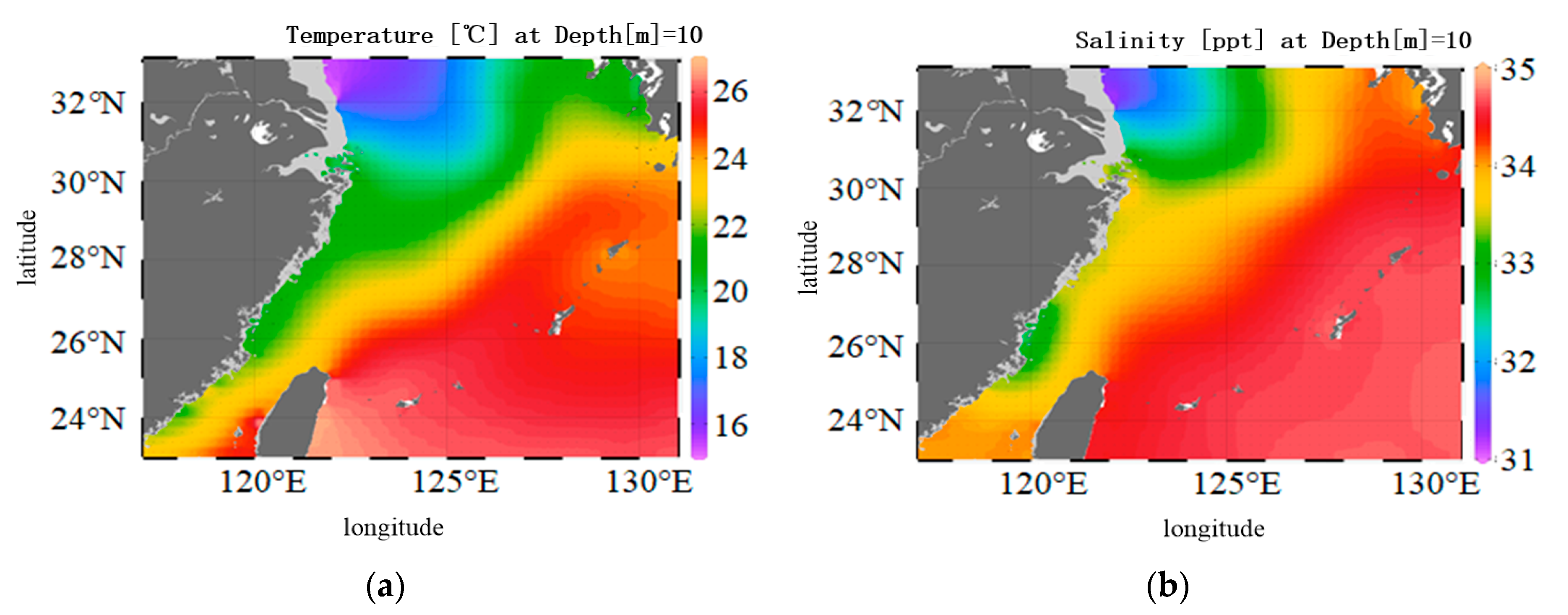
2.2. Hydrological Data of the East China Sea Area

To obtain true temperature and salinity data, hydrological data from the East China Sea area were used. The study area is located between 23°00′ and 33°10′ north latitude and 117°11′ and 131°00′ east longitude. The temperature and salinity distribution data of the East China Sea area from 2017 at a water depth of 10 m were obtained from the world marine environment database (WOA18) [20] and viewed using ocean data view (ODV 5.7.1) software, as shown in Figure 1.
As shown in Figure 2, at a depth of 10 m in the East China Sea, the seawater temperature ranges from 15.0 °C to 26.5 °C, and the seawater salinity ranges from 31.0 ppt to 35.0 ppt. The relationship of the refractive index n ( T , S , λ ) between temperature and salinity is shown in Figure 2.
The median of the temperature and salinity range in the East China Sea is considered the average temperature and salinity, that is T = 22.8 °C and S = 33.0 ppt, so the average refractive index of seawater and the linear coefficient are obtained, that is, n = 1.341, A = 1.05 × 10 4 L/deg, and B = 1.85 × 10 4 L/g.

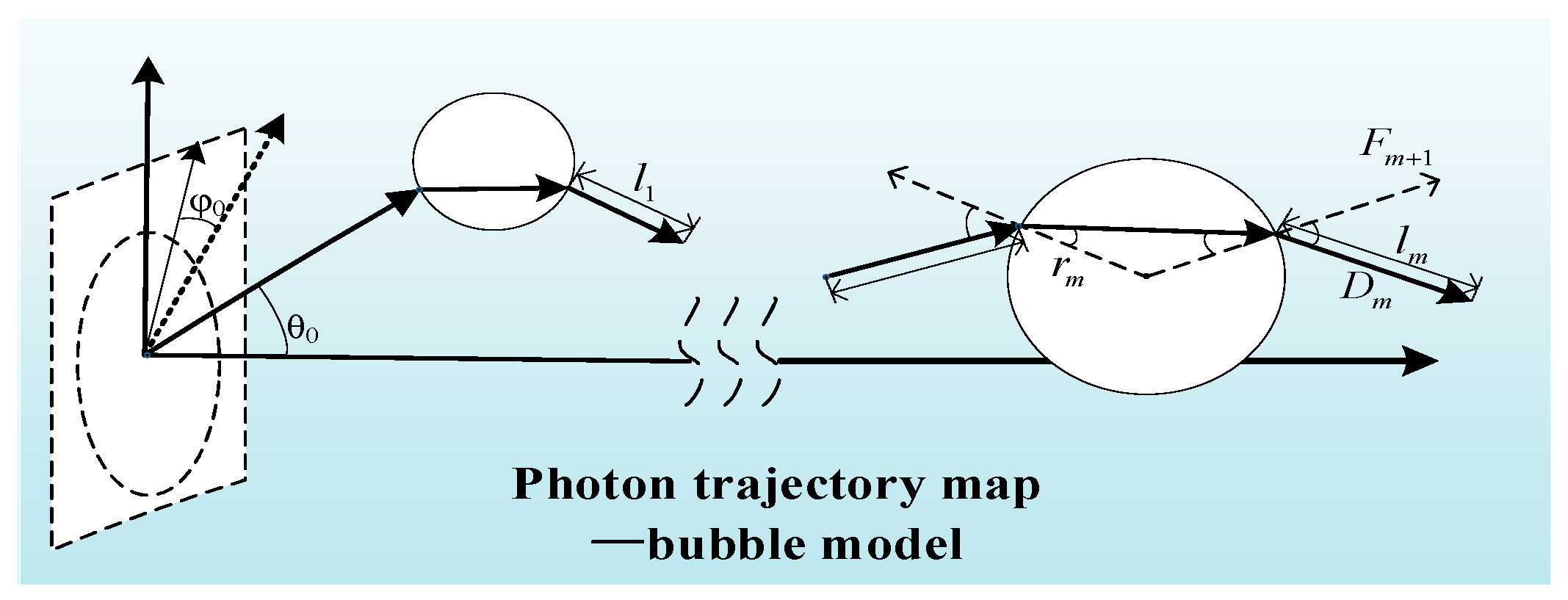
2.3. Establishment of a Bubble Simulation Model for the Ocean Turbulence Channels

According to Kolmogorov’s turbulence structure energy theory, initial turbulence energy is composed of large-scale vortex elements. When the turbulence velocity increases to a certain value, the large-scale vortex elements are immediately decomposed into small-scale vortex elements. As the velocity of the fluid decreases to a certain extent and the energy of the vortex element becomes insufficient to continue splitting downwards, the splitting stops immediately. At this point, the scale of the maximum vortex element is the outer scale of turbulence, denoted by L 0 , while the scale of the minimum vortex element is the inner scale of turbulence, denoted by η . A schematic diagram of the turbulent structure energy levels proposed by Kolmogorov is shown in Figure 3.
A large number of vortex elements in seawater have different refractive index fluctuation levels and sizes. Therefore, based on a random interface geometrical optics model, the activity of a single photon passing through a turbulent vortex element can be abstracted as the continuous multiple refraction phenomenon of a photon passing through a turbulent bubble with different refractive indexes and sizes, where the radius of the bubble is between the inner and the outer scales of turbulence. As a result, the photons passing through the turbulent channel experience different motion trajectories, displacements, and times, which affect the transmission characteristics of optical signals. Using the Monte Carlo simulation method, we established a turbulent bubble simulation model to study the propagation characteristics of the beam in a turbulent ocean channel, as shown in Figure 4, which is determined by the coordinates of the incident point, the radius, and the refractive index of the bubble.
The transmitter uses the Gaussian beam mode in Figure 5, which is the initial position P 0 x 0 , y 0 , z 0 and direction vectors D 0 μ x 0 , μ y 0 , μ z 0 of the photons that meet the Gaussian distribution. In the three-dimensional coordinate system, the photons transmission directions are in the Z-direction, and Figure 5 is a three-dimensional schematic diagram of the photon trajectory.
The refractive index inside the turbulent bubble n i ( n 1 , n 2 ) follows a Gaussian distribution [15] N n , Δ n 2 , where the average refractive index in the East China Sea is n , while Δ n is the standard deviation of the seawater refractive index fluctuations. The radius of the turbulent bubble is defined as r i , which follows the uniform distribution U η , L 0 . The transmission distance of the photons between the exit point of the previous bubble and the entrance point of the next bubble is the free path of turbulent transmission l i i = 1 , 2 , , which follows the Gaussian distribution N l b , Δ l b 2 .
According to the 3 σ principles, for a sample of data following a Gaussian distribution—N(μ, σ), the probability that the values fall within the range of (μ − σ, μ + σ) is 68.3%; the probability that the values fall within the range of (μ − 2σ, μ + 2σ) is 95.4%; and the probability that the values fall within the range of (μ − 3σ, μ + 3σ) is 99.7%. Here l b is the mean and Δ l b is the standard deviation of the free path of turbulent transmission, in which the density function is symmetric about the mean l b . Therefore, the 99.7% area is in the interval l b 3 Δ l b , l b + 3 Δ l b ; the PDF distribution curve of the free path of turbulent transmission l i is shown in Figure 6.
To improve computational efficiency and ensure that the l i is positive, we apply the constraint l b = 3 Δ l b , and the l b should be much larger than the inner scale of turbulence η . When simulating the interaction between the photons and the turbulent bubble, due to the different refractive indices of the inside medium and the outside medium of the turbulent bubble, it is necessary to determine the interactions between the photons and the turbulent bubble medium on the transmission path including total reflection, reflection, and refraction.
1 n / n b × sin θ i n 2 < 0 ,
θ i n is the angle between the incident direction D and the normal F; that is, the total reflection condition is met. Next, the photon undergoes total reflection on the surface of the turbulent bubble, and the photon’s present direction vector is D + 2 cos θ i n × F .
In addition to total reflection, reflection or refraction between photons and spherical bubbles are also possible. Based on Fresnel’s refraction theorem [16], the reflection and transmission coefficients of the s-component are as follows:
γ s = sin θ i n θ o u t sin θ i n + θ o u t ,
t s = 2 cos θ i n sin θ o u t sin θ i n + θ o u t .
The reflection and transmission coefficients of the p-component are as follows:
γ p = tan θ i n θ o u t tan θ i n + θ o u t ,
t p = 2 cos θ i n sin θ o u t sin θ i n + θ o u t cos θ i n θ o u t ,
θ o u t is the angle between the direction of refraction or reflection RD and the normal F. Because of the equal energy of the s wave and the p wave, the reflectivity is γ = γ s 2 + γ p 2 / 2 , γ + t = 1 , and t is the transmission coefficient. To determine whether a refraction phenomenon or a reflection phenomenon is occurring the γ and ς of a uniformly distributed random number between 0 and 1 are compared. When ς γ , it is determined that the reflection phenomenon occurs between photons and the turbulent bubble, and the outgoing direction vector is the same as the total reflection; otherwise, it is refraction.
When n < n b , sin θ in > n b / n and ς > γ , photons are refracted into the m-th turbulent bubble. The initial point coordinates of photons leaving the (m − 1)-th turbulent bubble are P m 1 x m 1 , y m 1 , z m 1 , the displacement of exiting the (m − 1)-th turbulent bubble and entering the m-th turbulent bubble is the free path of turbulent transmission l m 1 , and the direction vector is D m 1 μ x m 1 , μ y m 1 , μ z m 1 . Therefore, it is possible to uniquely determine the tangent point coordinate P m x m , y m , z m between the photon trajectory and the m-th turbulent bubble, expressed as follows:
P m : x m = x m 1 + l m 1 · μ x m 1 y m = y m 1 + l m 1 · μ y m 1 z m = z m 1 + l m 1 · μ z m 1 ,
The refractive index of the m-th turbulent bubble is n m , due to the difference between the internal refractive index of the turbulent bubble and the refractive index of the outer seawater medium, photons undergo two refractions in their trajectory while entering and exiting the bubble. According to the three-dimensional spatial structure, the coordinates of the center of the sphere O m can be uniquely determined by the coordinate points of the incident bubble P m , the incident normal F m , and the radius of the turbulent bubble r m . The coordinates of the center of the sphere are as follows:
O m = P m F m × r m ,
where the incident normal vector F m is determined by the scattering angle θ and azimuth angle φ , θ 0 , 2 π , φ 0 , 2 π , according to the principle of vector transformation, to satisfy the photon trajectory passing through the turbulent bubble, the photon trajectory must be met at D m 1 × F m T 0 , otherwise the photon trajectory deviates from the turbulent bubble. Photons refract through the tangent point P m and enter the m-th turbulent bubble, the length of the transmitted path in the m-th turbulent bubble is l m = 2 cos θ o u t × r m , and the direction of the photon motion inside the turbulent bubble after refraction is R D m :
R D m = M 1 D m 1 + M 2 F m ,
where M = cos θ i n 1 1 cos θ o u t 1 cos θ o u t cos θ i n θ o u t .
Table 1 lists the definition of parameters. Based on the bubble model established above, using the parameters in Table 1, the impact of ocean turbulence channels of large-scale ocean turbulence vortices on underwater wireless optical communication performance can be simulated.

3. Simulation Analysis of the Bubble Simulation Model for Turbulent Ocean Channels

3.1. Distribution of the Light Intensity Probability Density Function

In order to analyze optical characteristics in the turbulent ocean channel, we studied the PDF of the received light intensity. Using the spherical bubble simulation model at different outer scales L 0 , with the photon number set to 10 6 , a fundamental mode Gaussian light source with a beam radius of 1 cm and a wavelength is 532 nm, and where n was 1.341, Δ n was 0.002, l b was 5 m, Δ l b was 5/3 m, and η was 0.001 m, we obtained the PDF fitting curves of light intensity at the receiving end by using the bubble simulation model in multiple Monte Carlo simulations under different outer scales and different transmission distances, as shown in Figure 7a,b.
In the region of weak fluctuations, the statistics of the irradiance fluctuations were found to obey the log-normal distribution, which is
p I = 1 I σ I 2 π exp ( ln I / I 0 + σ I 2 / 2 2 2 σ I 2 ) ,
where σ I 2 L is the scintillation index. which σ I 2 L is less than 1 in the region of weak fluctuations, and the received light intensity I is normalized by the average light intensity I 0 .
From Figure 7a, it can be seen that the PDF obtained from the Monte Carlo simulation is in good agreement with the logarithmic normal curve, which can prove the effectiveness of the spherical bubble simulation model for ocean turbulence channels. Figure 7a shows that the impact of turbulence on the light intensity becomes greater as the L 0 becomes smaller, while from Figure 7b, it can be seen that the impact of turbulence on the light intensity increases greater as L increases. From Figure 7a,b, the shape of the PDF curve indicates that the transmission distance has a greater impact on the fluctuation in light intensity compared to the outer scale.
Specific data on the impact of different outer scales and transmission distances on the scintillation index are shown in Table 2. By comparing the numerical results in Table 2, it can also be concluded that the influence of the outer scale on the light intensity fluctuations is greater than that of the transmission distance.

3.2. The Influence of the Turbulent Bubble Parameters on Fluctuations on the Light Intensity

After verifying the correctness of the bubble simulation model for the turbulence channel, in order to obtain the fluctuation in the received light intensity, we assumed that the emitted laser is aligned with the receiver, and the emitted light intensity is affected by ocean turbulence, resulting in fluctuations in light intensity at the receiving end. The equation for the scintillation index of the received light intensity at the receiving end is as follows [21]:
σ I 2 L = I 2 L I L 2 1 .
The Monte Carlo simulation parameters were a photon number of 10 6 , collimation Gaussian beam width of 1 cm, n = 1.341, and η = 10 3 m. The standard deviations of refractive index fluctuations of seawater were Δ n = 5 × 10 4 , Δ n = 10 3 , and Δ n = 2 × 10 3 . The average free path values were l b = 3 m, l b = 5 m, and l b = 7 m, respectively. The outer scales are L 0 = 3 m, L 0 = 5 m, and L 0 = 7 m. The variation curves of the intensity fluctuations at different L 0 and L values of 20 to 40 m are shown in Figure 8a; Figure 8b shows the variation curves of the intensity fluctuation at L values of 20 m to 40 m under different Δ n ; and the variation curves of the intensity fluctuation at L of 20 m to 40 m values under different l b are shown in Figure 8c.
The simulation results from Figure 8a show that the fluctuation of the light intensity increases with an increase in the link distance L at the same outer scale L 0 of ocean turbulence, and the light intensity fluctuation trend is approximately a cubic function curve with L. The fluctuation in the light intensity decreases with an increase in L 0 at the same L. This is because a larger L 0 will reduce the number of bubbles existing in the turbulent channel within a certain link distance, as well as the chance of photons interacting with the turbulent bubble. When L is 40 m, the light intensity fluctuation caused by an L 0 of 3 m is approximately 1.566 times that caused by an L 0 of 7 m; when L 0 is 5 m, the light intensity fluctuation caused by an L of 40 m is approximately 24.684 times that of an L of 20 m, showing that L has a greater impact on the fluctuation of the light intensity.
The simulation results in Figure 8b show that the fluctuation in the light intensity increases with the increase an Δ n in the same L. According to Snell’s law, the larger the Δ n , the greater the angle between the direction vector of photon propagation inside the bubbles and the direction vector of the outgoing bubbles, the amplitude of photon trajectory change would be greater, which enhances the phenomenon of the light intensity fluctuation. Meanwhile, the longer the L of the link, the greater the impact of Δ n on the fluctuation in the light intensity. When L is 40 m, the fluctuation in the light intensity of Δ n = 2 × 10 3 is approximately 458.551 times that of Δ n = 2 × 10 3 . When Δ n = 1 × 10 3 , the light intensity fluctuation caused by an L of 40 m is approximately 24.684 times that of an L of 20 m, which shows that the refractive index fluctuation has a greater impact on the light intensity fluctuation, compared to L.
The simulation results in Figure 8c show that the fluctuation in the light intensity decreases as the l b increases at the same L. This is because the increases in l b makes the distance between adjacent interacting bubbles longer, resulting in fewer collision opportunities and reducing the impact of turbulence on photons. Meanwhile, the longer the link distance L, the more significant the impact of l b on the fluctuation in the light intensity. When L is 40 m, the fluctuation in the light intensity caused by l b = 3 m is approximately 3.507 times that of l b = 7 m; when l b is 5 m, the fluctuation in the light intensity caused by L = 40 m is approximately 24.684 times that caused by L = 20 m, which shows that the influence of L on the fluctuation in the light intensity is greater, compared to l b .

3.3. The Models of Logarithmic Intensity Variance with Turbulent Bubble Parameters

According to the relationship between the scintillation index σ I 2 L and logarithmic intensity variance σ I 2 :
σ I 2 L = exp σ l 2 1 .
Using expression (16) and simulating scintillation index σ I 2 L at different values of L 0 , Δ n , and l b , we can create a model to demonstrate the influence of the turbulent bubble parameters on σ I 2 . Setting l b = 5 m, Δ l b = 5/3 m, Δ n = 10−3, L = 40 m, the fitting curves between different values of L 0 and σ I 2 was obtained by the simulation.
From Figure 9, it can be concluded that in Cartesian coordinates, σ l 2 is inversely proportional to L 0 . The fitted σ l 2 is related to L 0 of the bubble as shown in Formula (17).
σ l 2 = 0.01764 × L 0 0.4886 .
It can be seen that the relationship between L 0 and σ l 2 can be obtained from Equation (17), when L 0 is [3 m~7 m]. Figure 10 shows the fitting curves of the refractive index standard deviations Δ n and the logarithmic intensity variances σ l 2 , when l b = 5 m, Δ l b = 5/3 m, L = 40 m, L0 = 5 m.
From Figure 10, it can be concluded that σ l 2 is proportional to Δ n , and the relationship between the fitted σ l 2 and Δ n is as follows:
σ l 2 = 8.883 × 10 8 Δ n 3.68 .
The relationship between Δ n and σ I 2 can be obtained from Equation (18), where Δ n is in the interval [ 5 × 10 4 ~ 2 × 10 3 ] . The fit curve of the mean free path l b and the logarithmic intensity variance σ I 2 is shown in Figure 11 when Set Δ n = 10−3, L = 40 m, L0 = 5 m.
From Figure 11, it can be concluded that σ l 2 is inversely proportional to l b , and the relationship between the fitted σ l 2 and l b is:
σ l 2 = 0.08284 × l b 1.446 .
It can be seen that l b and σ l 2 satisfies the relationship in Equation (19), when l b is in the interval [3 m~7 m].

3.4. The Relationship between Logarithmic Intensity Variance and Equivalent Structure Constants

Assuming the light source is a quasi-straight Gaussian beam, which can be approximated as a plane wave, the logarithmic intensity variance σ I 2 of plane waves under weak turbulence is related to parameters such as equivalent structural constants, distance, etc., and is expressed as follows [22]:
σ l 2 = 4 × 0.56 k 7 / 6 0 L C n 2 ( x ) × ( L x ) 5 / 6 d x ,
By studying the relationship in (20) between the equivalent structural constant C n 2 and the logarithmic intensity variance σ I 2 , the fitting curve is obtained as shown in Figure 12.
From Figure 12, the relationship between the fitted σ l 2 and C n 2 is:
σ l 2 = 4.773 × 10 9 C n 2 ,
Combining the expression of the relationship in (17) between σ l 2 and L 0 , the expression of the relationship in (18) between σ l 2 and Δ n , and the expression of the relationship in (19) between σ l 2 and l b , we can establish the models of the relationship between the parameters of the bubble model for the ocean turbulence channels L 0 , Δ n , l b and the equivalent structural constant C n 2 , shown in Equations (22)–(24):
C n 2 = 3.696 × 10 12 L 0 0.4886 ,
C n 2 = 0.186 × Δ n 3.68 ,
C n 2 = 1.736 × 10 11 l b 1.446 ,
where L 0 is in the range of [3 m~7 m], Δ n is in the range of [ 5 × 10 4 ~ 2 × 10 3 ] , and l b with the range of [3 m~7 m]. From Equations (22)–(24), we can conclude that the influence of L 0 and l b on C n 2 shows a negative correlation and the influence of Δ n on C n 2 shows a positive correlation. The equivalent structural constants representing ocean turbulence C n 2 in matrix form are the following:
C n 2 = B × B r T = 3.696 × 10 12 L 0 0.4886 0.186 × Δ n 3.68 1.736 × 10 11 l b 1.446 T × B r T ,
where B r is the coefficient matrix, when studying the relationship between C n 2 and L 0 , B r = (1,0,0); when studying the relationship between C n 2 and Δ n , B r = (0,1,0); and when studying the relationship between C n 2 and l b , B r = (0,0,1), so we can obtain the corresponding C n 2 of ocean turbulence by changing the parameters of the bubble model by applying the bubble simulation model of the ocean turbulence channels.

3.5. Comparison between Simulation Results and Theoretical Values of Transmission Characteristics in Bubble Models

In order to compare the transmission characteristics of the bubble simulation model with the theoretical values under the same turbulence intensity, we introduced the isotropic ocean turbulence equivalent structure constants [23]:
C n 2 = 3.044 π × 10 8 ε 1 / 3 ε T ω 2 k 7 / 6 L 11 / 6 × 0 L d z d κ x d κ y 1 + 2.35 η 1 / 3 κ x 2 + κ y 2 1 / 3 × P z , κ x , κ y P z , κ x , κ y + P z , κ x , κ y 2 × 1 exp κ x 2 + κ y 2 / κ 01 2 κ x 2 + κ y 2 11 / 6 × w 2   exp A T δ + exp A s δ 2 w   exp A T S δ .
Here P z , κ x , κ y = i k   exp 0.5 ( k L ) 1 i z ( L z ) κ x 2 + κ y 2 , and Φ n κ is the exponential Nikishov power spectrum model, expressed as:
Φ n κ = 0.388 × 10 8 ε 1 / 3 1 + 2.35 κ η 2 / 3 × ε T ω 2 κ 11 / 3 1 exp κ 2 / κ 01 2 × ω 2   exp A T δ + exp A S δ 2 ω e x p A T S δ ,
where κ is the spatial frequency, ε is the kinetic energy dissipation rate, ε T is the temperature variance dissipation rate, η is the turbulent inner scale, κ 01 = 4 π / L 0 , L 0 is the turbulent outer scale, ω represents the ratio of temperature induction to salinity induction to, δ = 8.284 κ η 4 / 3 + 12.978 κ η 2 , A T = 1.863 × 10 2 , A S = 1.9 × 10 4 , and A T S = 9.41 × 10 3 . Based on wave optics theory, the long-term beam spread is expressed as:
W L E = W 1 + T ,
where W = w 0 Θ 0 2 + Λ 0 2 1 / 2 , T = 4 π 2 k 2 L 0 1 0 κ Φ n ( κ ) × 1 exp Λ L κ 2 ξ 2 k d κ d ξ , Λ = Λ 0 / Θ 0 2 + Λ 0 2 . After the beam is transmitted through a turbulent channel, a beam drift phenomenon occurs, and the theoretical equation of the centroid drift is as follows:
r c 2 = 4 π 2 k 2 L × 0 1 0 κ Φ n ( κ ) H LS 1 exp Λ L κ 2 ξ 2 k d κ d ξ ,
where H LS = exp κ 2 w 0 2 Θ 0 + Θ 0 ξ 2 + Λ 0 2 1 ξ 2 , ξ is the normalized path coordinate in the transmission direction; w 0 represents the initial beam width; Λ 0 and Θ 0 represent the beam parameters at the transmitter, Θ 0 = 1 L / F 0 ; F 0 is the radius of the curvature of the wavefront; and the beam width of the collimated Gaussian beam is 1 cm, F 0 , where, Θ 0 = 1, Λ 0 = 2 L / k w 0 2 , and the wave vector k = 2 π / λ .
Based on the above analysis, when ε = 10 6 , ε T = 10 7 , η = 10 3 m, ω = −2, and L = 40 m, we obtained C n 2 = 1.3176 × 10 12 according to Equation (24). In the spherical bubble simulation model of ocean turbulence channels, when n = 1.341, η = 10 3 m, L 0 = 5 m, L = 40 m, l b = 5 m, and Δ l b = 5/3 m, from Equation (23), we can determine the corresponding standard deviation of the refractive index fluctuation Δ n = 9.3 × 10 4 when the constants of the ocean turbulence structure C n 2 = 1.3176 × 10 12 . Therefore, we obtained the parameter values of the equivalent structure constants, as shown in Table 3.
We calculated the beam propagation characteristics of the bubble simulation model using the long exposure radius:
W LE 2 = r 2 I x , y d x d y I x , y d x d y .
Next, we measured the degree of centroid shift of the light spot through the standard deviation of the centroid drift.
σ c = x c 2 + y c 2 ,
x c , y c are the centroid coordinates, x c = x I x , y d x d y I x , y d x d y , y c = y I x , y d x d y I x , y d x d y . When C n 2 = 1.3176 × 10 12 , we conducted a Monte Carlo simulation on the bubble model for the ocean turbulence channels to obtain I x , y , and used Equations (30) and (31) to statistically analyze the results of beam expansion and centroid drift, respectively. Under the parameters shown in Table 3, we used Equations (28) and (29) to calculate the theoretical values of optical properties, and the results are shown in Table 4.
Table 4 shows the results of beam spread and centroid drift calculated using wave optics theory compared with the results based on the turbulence channel bubble simulation model. We can see that the bubble model can simulate the ocean turbulence channels to a certain extent, showing the theory and simulation are linked by equivalent structural constants.

4. Conclusions

Referring to the known process of turbulent vortex formation, in this study, using a random interface geometric optical method, a Monte Carlo simulation model of spherical bubbles in ocean turbulence channels was proposed. Subsequently, based on the basic temperature and salinity data of the East China Sea, log-normal function fitting was carried out by counting the received light intensity in the Monte Carlo simulation, which verified the correctness of the Monte Carlo bubble simulation model in this situation. The fluctuation characteristics of the light intensity in the bubble model were studied, and their relationship with the structural constants was analyzed.
The research results show that the fluctuation in light intensity decreases with an increase in the outer scale and the free path of turbulent transmission, while it increases with an increase in the refractive index standard deviation. The influence of transmission distance on light intensity fluctuation is the greatest when compared with the outer scale, the refractive index fluctuation, and the free path. The logarithmic intensity variance is inversely proportional to the outer scale and the mean free path, while it is directly proportional to the standard deviation of refractive index fluctuations. Both the outer scale of the turbulent bubble and the mean free path of turbulent transmission show a negative correlation with the equivalent structure constant of ocean turbulence, whereas the standard deviation of the refractive index fluctuation of seawater shows a positive correlation with the equivalent structure constant of ocean turbulence. Finally, the simulation results of the optical parameters were compared with the calculation results of wave optics theory, further demonstrating that the spherical bubble model conforms to transmission theory.
The above research only considered the impact of relative refractive index and free path parameters in the bubble model on the underwater wireless optical communication performance. In the future, further research should be conducted on the relationship between the parameters of the bubble model and turbulence effects to study the impact of seawater channels under large-scale turbulence on the performance of underwater wireless optical communication.

Author Contributions

Conceptualization, Y.Z. and H.N., Methodology, Y.Y. and J.Z., Software, H.N. and Q.L. Investigation, Y.Z., Writing—original draft, H.N., Writing—review & editing, Q.L. All authors have read and agreed to the published version of the manuscript.

Funding

This research was funded by Foundation of the Ministry of Education for Equipment Advance Research, grant number (8091B032130) and National Key Research and Development Program Project, grant number (2023YFB2905602).

Data Availability Statement

Data is contained within the article.

Conflicts of Interest

The authors declare no conflict of interest.

References

  1. Saeed, N.; Celik, A.; Al-Naffouri, T.Y.; Alouini, M.S. Underwater optical wireless communications, networking, and localization: A survey. Ad Hoc Netw. 2019, 94, 101935. [Google Scholar] [CrossRef]
  2. Anous, N.; Abdallah, M.; Uysal, M.; Qaraqe, K. Performance evaluation of LOS and NLOS vertical inhomogeneous links in underwater visible light communications. IEEE Access 2018, 6, 22408–22420. [Google Scholar] [CrossRef]
  3. Vijayakumari, P.; Chanthirasekaran, K.; Jayamani, K.; Nirmala, P.; ThandaiahPrabu, R. BIT Error Rate Analysis of Various Water Samples in Underwater Wireless Optical Communication System. In Proceedings of the 2022 International Conference on Advances in Computing, Communication and Applied Informatics (ACCAI), Chennai, India, 28–29 January 2022; pp. 1–5. [Google Scholar]
  4. Liu, W.; Ye, Z.; Huang, N.; Li, S.; Xu, Z. Multilevel polarization shift keying modulation for turbulence-robust underwater optical wireless communication. Opt. Express 2023, 31, 8400–8413. [Google Scholar] [CrossRef] [PubMed]
  5. Lin, Z.; Xu, G.; Zhang, Q.; Song, Z. Average symbol error probability and channel capacity of the underwater wireless optical communication systems over oceanic turbulence with pointing error impairments. Opt. Express 2022, 30, 15327–15343. [Google Scholar] [CrossRef] [PubMed]
  6. Ji, X.; Yin, H.; Jing, L.; Liang, Y.; Wang, J. Modeling and performance analysis of oblique underwater optical communication links considering turbulence effects based on seawater depth layering. Opt. Express 2022, 30, 18874–18888. [Google Scholar] [CrossRef] [PubMed]
  7. Hill, R. Optical propagation in turbulent water. JOSA 1978, 68, 1067–1072. [Google Scholar] [CrossRef]
  8. Zhao, G.; Yan, Q.; Yu, L.; Hu, L.; Zhang, Y. Spatial coherence length and wave structure function for plane waves transmitted in anisotropic turbulent oceans. JOSA A 2023, 40, 1602–1611. [Google Scholar] [CrossRef] [PubMed]
  9. Lin, Z.; Xu, G.; Wang, W.; Zhang, Q.; Song, Z. Scintillation index for the optical wave in the vertical oceanic link with anisotropic tilt angle. Opt. Express 2022, 30, 38804–38820. [Google Scholar] [CrossRef] [PubMed]
  10. Cai, R.; Zhang, M.; Dai, D.; Shi, Y.; Gao, S. Analysis of the Underwater Wireless Optical Communication Channel Based on a Comprehensive Multiparameter Model. Appl. Sci. 2021, 11, 6051. [Google Scholar] [CrossRef]
  11. Pan, Y.; Wang, P.; Wang, W.; Li, S.; Cheng, M.; Guo, L. Statistical model for the weak turbulence-induced attenuation and crosstalk in free space communication systems with orbital angular momentum. Opt. Express 2021, 29, 12644–12662. [Google Scholar] [CrossRef]
  12. Li, Y.; Xie, Y.; Li, B. Probability of orbital angular momentum for square Hermite–Gaussian vortex pulsed beam in oceanic turbulence channel. Results Phys. 2021, 28, 104590. [Google Scholar] [CrossRef]
  13. Niu, C.; Wang, X.; Lu, F.; Han, X. Validity of beam propagation characteristics through oceanic turbulence simulated by phase screen method. Infrared Laser Eng. 2020, 49, 243–249. [Google Scholar]
  14. Baykal, Y. Expressing oceanic turbulence parameters by atmospheric turbulence structure constant. Appl. Opt. 2016, 55, 1228–1231. [Google Scholar] [CrossRef] [PubMed]
  15. Yuksel, H.; Atia, W.; Davis, C.C. A geometrical optics approach for modeling atmospheric turbulence. In Atmospheric Optical Modeling, Measurement, and Simulation; Yuksel, H., Atia, W., Davis, C.C., Eds.; SPIE: Bellingham, WA, USA, 2005; Volume 5891, pp. 77–88. [Google Scholar]
  16. Xue, Y.; Ma, L.; Shi, L.; Luo, J. Performance analysis of free space quantum key distribution based on refraction of turbulence bubble. Acta Photonica Sin. 2017, 46, 36–41. [Google Scholar]
  17. Chen, C.; Yang, H.; Feng, X.; Fan, J.; Wang, H.; Han, C.; Ding, Y. Monte Carlo simulation of beam wander in atmospheric turbulence based on spherical bubble model. J. Chang. Univ. Sci. Technol. (Nat. Sci. Ed.) 2008, 31, 4. [Google Scholar]
  18. Quan, X.; Fry, E.S. Empirical equation for the index of refraction of seawater. Appl. Opt. 1995, 34, 3477–3480. [Google Scholar] [CrossRef]
  19. Yao, J.R.; Elamassie, M.; Korotkova, O. Spatial power spectrum of natural water turbulence with any average temperature, salinity concentration, and light wavelength. J. Opt. Soc. Am. A Opt. Image Sci. Vis. 2020, 37, 1614–1621. [Google Scholar] [CrossRef]
  20. Xu, N.; Zhang, B.; Luo, N. Simultaneous inversion of seawater temperature and salinity based on stimulated brillouin scattering. Acta Opt. Sin. 2022, 42, 2429001. [Google Scholar]
  21. Baykal, Y. Intensity fluctuations of multimode laser beams in underwater medium. JOSA A 2015, 32, 593–598. [Google Scholar] [CrossRef]
  22. Benton, D.M.; Ellis, A.D.; Li, Y.; Hu, Z. Emulating atmospheric turbulence effects on a micro-mirror array: Assessing the DMD for use with free-space-to-fibre optical connections. Eng. Res. Express 2022, 4, 045004. [Google Scholar] [CrossRef]
  23. He, F.; Du, Y.; Zhang, J. Bit error rate of pulse position modulation wireless optical communication in gamma-gamma oceanic anisotropic turbulence. Acta Phys. Sin. 2019, 68, 236–244. [Google Scholar] [CrossRef]
Figure 1. Temperature and salinity distribution in the East China Sea at 10 m water depth: (a) temperature distribution; (b) salinity distribution.
Electronics 13 02626 g001
Figure 2. Changes in the refractive index of seawater with temperature and salinity: (a) refractive index changes with temperature; (b) refractive index changes with salinity.
Electronics 13 02626 g002
Figure 3. Schematic diagram of the turbulent structure energy levels.
Electronics 13 02626 g003
Figure 4. Bubble simulation model for turbulent channel based on refractive index fluctuation.
Electronics 13 02626 g004
Figure 5. Three-dimensional photon trajectory in a bubble model.
Electronics 13 02626 g005
Figure 6. Gaussian probability density function curve of the free path.
Electronics 13 02626 g006
Figure 7. PDF curves at different transmission distances and outer scales: (a) different outer scales; (b) different transmission distance.
Electronics 13 02626 g007
Figure 8. Scintillation index under different bubble parameters: (a) different outer scales; (b) different standard deviations of refractive index; (c) different free paths of transmission.
Electronics 13 02626 g008aElectronics 13 02626 g008b
Figure 9. Fitting curve of the outer scale and the logarithmic strength variance.
Electronics 13 02626 g009
Figure 10. Fitting curve between the standard deviation of refractive index fluctuation and the logarithmic intensity variance.
Electronics 13 02626 g010
Figure 11. Fit curve of the mean free path and the logarithmic strength variance in transmission.
Electronics 13 02626 g011
Figure 12. Fitting curve between equivalent structural constant and logarithmic strength variance.
Electronics 13 02626 g012
Table 1. Parameter definition for the bubble model in seawater turbulence channels.
ParameterParameter Definition
nrefractive index under average T and S in the East China Sea
Δ n the standard deviation of the refractive index fluctuations
η the minimum ocean turbulence vortex scale
L 0 the largest ocean turbulence vortex scale
l b the mean free path of turbulent transmission
Δ l b the standard deviation of the free path
Nthe total number of simulated photons
Ltransmission distance
Table 2. The influence of the outer scale and transmission distance on the scintillation index.
L 0 Change
(L = 40 m)
Scintillation Index
σ I 2 L
L Change
( L 0 = 5 m)
Scintillation Index σ I 2 L
3 m0.130720 m0.0083
5 m0.109830 m0.0401
7 m0.088140 m0.1098
Table 3. Transmission characteristics comparison of the parameter values.
ParameterValueParameter Definition
Theoretical Calculation ε 10 6 dissipation rate of Kinetic Energy
ω −2Thermohaline diffusion ratio
ε T 10 7 dissipation rate of temperature variance
η 0.001 mthe minimum ocean turbulence vortex scale
L 0 5 mthe largest ocean turbulence vortex scale
Δ z 5 mthe spacing between phase screens
Turbulent Bubble Simulation Modeln1.341refractive index under average T and S
n 0.00093standard deviation of refractive index fluctuations
Δ l b 5/3 mthe standard deviation of the free path
η 0.001 mthe minimum ocean turbulence vortex scale
L 0 5 mthe largest ocean turbulence vortex scale
l b 5 mthe mean free path of turbulent transmission
Table 4. Comparison of theoretical and simulated transmission characteristics.
Transmission CharacteristicsTheoretical CalculationBubble Model
Beam expansion (cm)1.05691.0523
Centroid drift (cm)0.12800.1245
Disclaimer/Publisher’s Note: The statements, opinions and data contained in all publications are solely those of the individual author(s) and contributor(s) and not of MDPI and/or the editor(s). MDPI and/or the editor(s) disclaim responsibility for any injury to people or property resulting from any ideas, methods, instructions or products referred to in the content.

