Anomaly Detection Based on GCNs and DBSCAN in a Large-Scale Graph

Abstract

Anomaly detection is critical across domains, from cybersecurity to fraud prevention. Graphs, adept at modeling intricate relationships, offer a flexible framework for capturing complex data structures. This paper proposes a novel anomaly detection approach, combining Graph Convolutional Networks (GCNs) and Density-Based Spatial Clustering of Applications with Noise (DBSCAN). GCNs, a specialized deep learning model for graph data, extracts meaningful node and edge representations by incorporating graph topology and attribute information. This facilitates learning expressive node embeddings capturing local and global structural patterns. For anomaly detection, DBSCAN, a density-based clustering algorithm effective in identifying clusters of varying densities amidst noise, is employed. By defining a minimum distance threshold and a minimum number of points within that distance, DBSCAN proficiently distinguishes normal graph elements from anomalies. Our approach involves training a GCN model on a labeled graph dataset, generating appropriately labeled node embeddings. These embeddings serve as input to DBSCAN, identifying clusters and isolating anomalies as noise points. The evaluation on benchmark datasets highlights the superior performance of our approach in anomaly detection compared to traditional methods. The fusion of GCNs and DBSCAN demonstrates a significant potential for accurate and efficient anomaly detection in graphs. This research contributes to advancing graph-based anomaly detection, with promising applications in domains where safeguarding data integrity and security is paramount.

1. Introduction

Anomaly detection, also called outlier detection, is the identification of rare items, observations, or events that do not conform to the general patterns or behaviors of most of the data [1]. Detecting anomalies before analyzing data is an important task to ensure data quality, prevent fraud and security breaches, and resolve issues before they cause significant damage [2,3,4]. With the proliferation of digital technologies, organizations now have access to vast amounts of data from a variety of sources, including sensors, IoT devices, social media, and transactional systems, which provide fertile ground for detecting anomalies and gaining valuable insights. These data can be represented in complicated data structures such as graphs, making it difficult to detect anomalies.

Detecting anomalies in a graph requires using a feature extraction method or a representation learning method to extract relevant features from node attributes or the structure of the graph [1,4,5,6]. Various anomaly detection methods have been proposed to detect anomalies in large graphs, such as cluster-based anomaly detection [7,8], outlier detection algorithms [9], and deep learning anomaly detection [10,11]. A commonly used clustering method for anomaly detection is DBSCAN [12,13], which clusters data points that are close to each other in a high-dimensional space. DBSCAN specifies a minimum distance between points and a minimum number of points within that distance to be considered a cluster. However, finding the optimal value of these hyper parameters is an important task because it directly affects the clustering results.

With the growth of communication technologies, the volume of data can reach trillions of useful information that needs to be processed efficiently. Several studies have been conducted on processing information from large graphs, especially with the goal of detecting unusual behavior in the network [7,8,9,10,11]. Depending on how the data are collected, there are many types of anomalies in graphs, such as anomalous nodes, anomalous edges, anomalous subgraphs, and change detection [1,14,15]. The development of the Internet has made searching and sharing information fast and efficient. As the world grows into a fully interconnected structure, detecting anomalies in large graphs is a major challenge. The purpose of representing data with a graph is to summarize and display the information in each dataset, and particularly the key properties, while strictly maintaining the integrity of the representation of the dataset. This task can be helpful both in analyzing the data and in communicating the results. Errors or mistakes in huge datasets, resulting in anomalous nodes and patterns in large graphs, can have a significant impact on the expected outcome of a given task. The detection of such anomalous patterns is necessary to ensure a high success rate for the task being performed.

Many approaches have been developed and discovered to identify abnormal behavior in large graphs. The traditional approach to identify abnormal behavior uses the concept of change detection, which consists of finding the normative patterns in the data and then detecting abnormal objects that deviate significantly from the norm [5,14]. Other methods have been proposed with a feature-based approach, which uses graph representation to extract structural graph-centric features for outlier detection [9,16]. However, these conventional methods omit the graph labeled information which also provides insightful information for anomaly detection, limiting their effectiveness. Nowadays, the proposed methods enable the detection of network information using deep learning [3,4], which learns from node features, as well as from their relationships. Another recent anomaly detection method is to compute an anomaly score for each node and consider the nodes with the highest anomaly score as abnormal, while normal nodes have the lowest anomaly score [17]. Despite these advancements, challenges remain, including scalability concerns and the interpretability of results.

To address these limitations, this paper proposes a novel approach that integrates labeled information, automatic feature extraction through GCNs, and a scalable clustering technique such as DBSCAN to provide improved accuracy, scalability, and interpretability in detecting anomalies in large graphs. The combination of GCNs and DBSCAN for anomaly detection leverages the strengths of both methods to improve detection accuracy. GCNs are effective at capturing complex relationships and patterns in graph-structured data and provide a meaningful representation of the dataset, while DBSCAN excels at identifying clusters of different shapes and sizes and is robust to noise, making it suitable for detecting anomalies as points that do not fit well into a cluster. By integrating GCNs to preprocess and enrich the data representation and then applying DBSCAN to this improved representation, the approach can better distinguish between normal and abnormal patterns, leading to more reliable anomaly detection. Our contributions can be summarized as follows:

• We exploit the ability of GCNs to capture the structural information of the graph and the underlying patterns by using two convolutional layers. We encode the output of the GCNs into two vectors, representing the mean of the distribution ($\mathrm{z}\_\mathrm{m}\mathrm{e}\mathrm{a}\mathrm{n}$) and the logarithm of the variance of each dimension ($\mathrm{z}\_\mathrm{l}\mathrm{o}\mathrm{g}\_\mathrm{v}\mathrm{a}\mathrm{r}$). Together, these vectors form a two-dimensional representation that defines a multivariate normal distribution in latent space.
• We present a heuristic approach for the automatic determination of the hyperparameter epsilon in DBSCAN that eliminates the need for manual intervention. Through empirical evaluation on real-world datasets tailored for anomaly detection, we demonstrate the effectiveness of our method. Our experiments emphasize the superiority of our approach in efficiently detecting anomalies in large graph structures.

The remainder of this paper is organized as follows. Section 2 gives an overview of the work covered in this paper. Section 3 describes the details of the proposed method for detecting anomalies in large graphs. In Section 4, we verify the performance of our method using various performance evaluation results. Finally, Section 5 presents the conclusions, limitations, and future research directions.

2. Related Work

In response to the inherent complexity of graph data, researchers have made considerable efforts to develop techniques to represent such high-dimensional data in low-dimensional vector spaces. This endeavor, known as graph embedding, aims to distill the rich structural information contained in graphs while reducing their dimensionality. In parallel to graph embedding, the use of clustering methods has proven to be a powerful approach for detecting anomalies and uncovering underlying patterns in low-dimensional representations of graphs. Clustering algorithms play a crucial role in partitioning data points into coherent groups based on similarity or proximity, facilitating the identification of meaningful clusters and outliers in embedded graph representations.

2.1. Graph Embedding Approaches

Graph embedding approaches that aim to preserve the structural properties and relational information of the graph while reducing the dimensionality of node representations include node2vec [18], DeepWalk [19], LINE (Large-scale Information Network Embedding) [20], SDNE (Structural Deep Network Embedding) [21], GraphSAGE (Graph Sample and Aggregation) [22], and GCNs (Graph Convolutional Networks) [23].

Node2vec, presented by Grover and Leskovec (2016), uses random walks to generate node sequences, which are then used to train a skip-gram model to learn node embeddings. By balancing exploration and exploitation during the generation of random walks, node2vec effectively captures both local and global graph structures.

DeepWalk, proposed by Perozzi et al. (2014), uses truncated random walks to extract node sequences from graphs and uses skip-gram or another language modeling technique to learn node embeddings. DeepWalk efficiently captures the structural information of graphs by treating the random walks as sentences and the nodes as words.

LINE, introduced by Tang et al. (2015), learns node representations by preserving both the local and global network structures. By optimizing the first- and second-order proximities of nodes in the embedding space, LINE achieves scalable and efficient embedding generation for large networks.

SDNE, proposed by Wang et al. (2016), incorporates an autoencoder-based framework for learning node representations. By preserving the proximity of first- and second-order nodes while minimizing reconstruction errors in the embedding space, SDNE effectively captures both the local and global structural information of graphs.

GraphSAGE, introduced by Hamilton et al. (2017), uses inductive representation learning by sampling and aggregating neighborhood information. By utilizing the sampled subgraphs and a trainable aggregator function, GraphSAGE generates node embeddings that capture the features and structural properties of the nodes in a scalable manner.

GCNs, proposed by Kipf and Welling, extend convolutional neural networks to graph-structured data. By aggregating information from a node’s neighborhood using graph convolutional layers, GCNs capture both local and global graph structures and achieve peak performance on various graph-based tasks.

2.2. Clustering Algorithms for Anomaly Detection

Clustering for anomaly detection in graphs uses the inherent structure of the data to distinguish between normal and abnormal behavior, enabling timely detection and response to potential threats or irregularities within the graph. Clustering methods, such as K-means clustering, DBSCAN (Density-Based Spatial Clustering of Applications with Noise), OPTICS (Ordering Points to Identify the Clustering Structure), mean shift clustering, and spectral clustering [24], have been used to detect anomalies in graph data in various contexts and applications and have proven their effectiveness.

K-means clustering is often used for anomaly detection in graph data. In the context of graphs, K-means clustering is often applied to node embeddings, obtained using techniques such as node2vec or GraphSAGE. For example, Makarov et al. [25] applied K-means clustering to node embeddings to detect anomalies in networks. By clustering nodes based on their embeddings and identifying clusters with significantly fewer members, they were able to locate anomalous nodes that represent potentially malicious users or bot accounts.

DBSCAN has been shown to be effective in identifying anomalies in graph data by clustering densely connected regions and labeling sparse regions as noise. Several studies have used DBSCAN for anomaly detection in network data [12,13,24]. For graph data, DBSCAN has been adapted to detect outliers or anomalies in connectivity patterns. Some researchers have proposed modified DBSCAN algorithms tailored to graph data that effectively identify outliers in large network graphs by considering both local and global density features.

OPTICS, an extension of DBSCAN, provides improved scalability and flexibility for detecting anomalies in graphs. By ordering points based on their reachability density, OPTICS can reveal the hierarchical structure of clusters and thus aid in anomaly detection. It has been used, for example, to detect anomalies in dynamic graph data such as evolving social networks. The hierarchical cluster structure generated by OPTICS enabled anomaly detection at multiple levels of granularity, accounting for the evolving nature of the graph.

Mean shift clustering is effective in identifying dense regions in graph data and is therefore suitable for anomaly detection. In the context of graph anomaly detection, mean shift has been used to detect anomalous subgraphs or communities with different connectivity patterns. For example, mean shift clustering has been used to detect anomalies in communication networks by identifying groups of nodes that exhibit unusual communication behavior. The adaptive nature of mean shift enabled the detection of anomalies without a priori assumptions about cluster shapes.

Spectral clustering has gained prominence for detecting anomalies in graph data due to its ability to capture the underlying structure of graphs. By partitioning the graph based on spectral properties, spectral clustering can identify anomalies such as nodes or subgraphs that deviate from the expected structural patterns. Spectral clustering has been applied on Laplacian embeddings of graphs to detect anomalies in financial transaction networks. Spectral decomposition revealed subtle structural anomalies indicative of fraudulent activity, outperforming traditional anomaly detection methods.

Although the existing clustering algorithms mentioned above are effective in partitioning datasets based on different perspectives and data types, it is difficult to find a single algorithm that is suitable for all situations. Each algorithm has its strengths and weaknesses, and its performance may vary depending on the characteristics of the dataset. This difficulty in finding an optimal clustering approach has led to the development of clustering ensemble methods. These methods combine results from different clustering algorithms or from multiple runs of the same algorithm with different parameters to achieve more robust and reliable results [26,27,28].

3. Proposed Anomaly Detection Method

In this section, we first give an overview of the proposed method, followed by embedding the graph and detecting anomalies using an automated DBSCAN.

3.1. Overall Structure

Since graphs are inherently high-dimensional, especially when considering the features associated with the nodes and edges, managing and processing graph data pose challenges for anomaly detection algorithms. Moreover, large graphs may contain noise or outliers that can mask true anomalies. Distinguishing between true anomalies and noise is a challenge, especially in graphs with sparse or noisy data. To tackle anomaly detection in large graphs, anomaly detection methods use different strategies, from rule-based or heuristic methods to machine learning. While rule-based methods rely on predefined rules, thresholds, or heuristics to detect anomalies in the data, anomaly detection methods that rely on machine learning use algorithms and models to automatically learn patterns and features of normal behavior from labeled or unlabeled data.

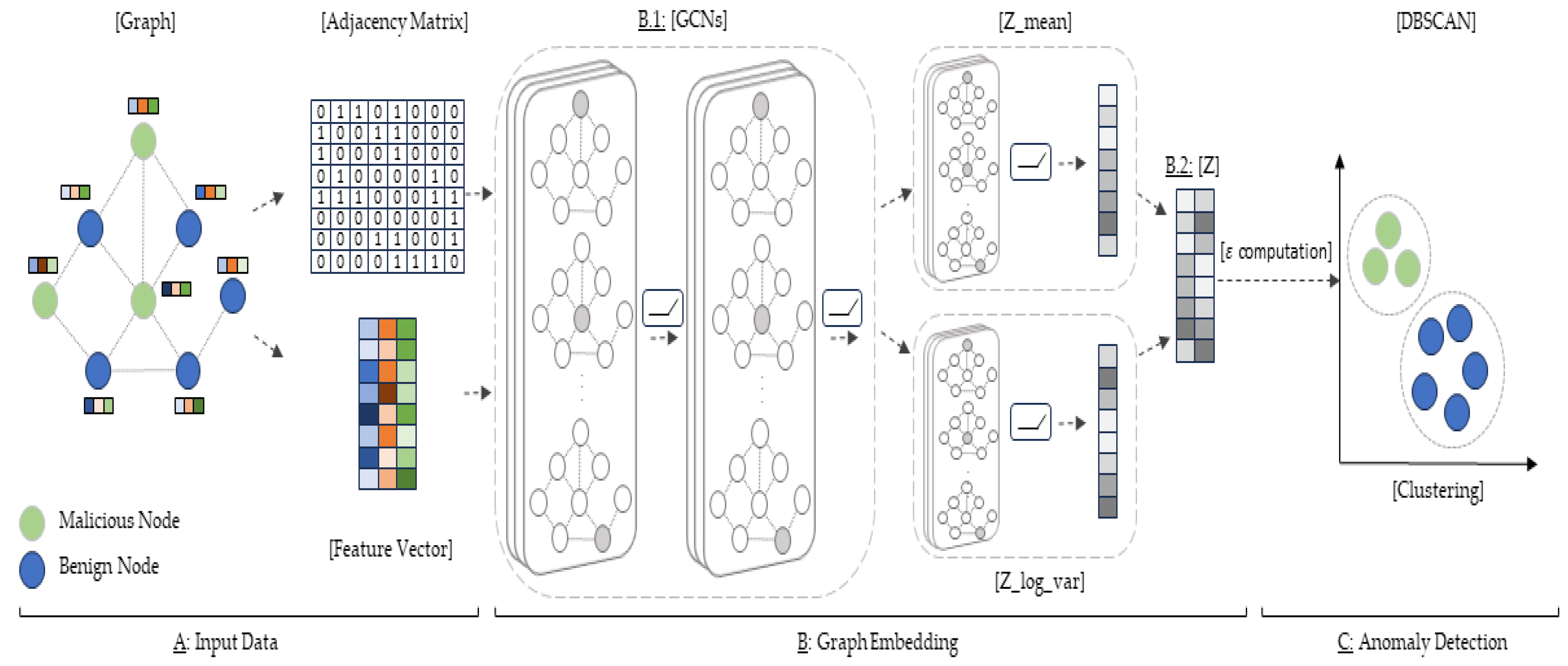
Figure 1 shows the overall structure of the proposed method. Given an undirected static graph with node features $G=\left\{N,E,F\right\}$, $N=\left\{n_1,n_2, n_3,\dots \right\}$ is the node set, $E=\left\{e_1, e_2, e_3,\dots \right\}$ is the edge set, and $F=\left\{f_1, f_2, f_3, \dots \right\}$ is the attribute set of each node. The proposed method first encodes the nodes of the graph in a continuous vector space by the graph embedding module (Figure 1B). The graph embedding module is divided into two parts. Since the node identity information in a graph is very important, we use GCNs that learn to map each node or the entire graph into a low-dimensional vector space by capturing their local and global structures and allowing the detection of features of neighboring nodes (Figure 1(B.1)). The nodes’ low-dimensional vector is then passed to a variational model that calculates the mean and log variance of each node (Figure 1(B.2)), resulting in the final graph embedding, represented in a two-dimensional vector. The output of the graph embedding is fed into the clustering module (Figure 1C) to find normal and abnormal nodes. Specifically, we use DBSCAN to automatically classify whether a node is abnormal or not.

3.2. Graph Embedding

Our method combines GCNs and multivariate normal distribution for graph embedding. GCNs capture structural information, while the normal distribution (or Gaussian distribution) is defined by two variables, such as the mean and the variance, to transform the graph into a two-dimensional latent representation.

3.2.1. Graph Convolutional Networks (GCNs)

GCNs are a class of neural networks developed for processing graphically structured data. They extend the concept of convolutional neural networks (CNNs) to graphs and allow information to be passed between nodes in a graph. In this work, we use two hidden layers to learn node features and graph structures according to the graph $G$. In graph-structured data, nodes represent entities, and edges represent relationships or connections between these entities. GCNs aim to learn node representations by capturing both local and global graph information. The input for a GCN model usually consists of two main components: node features and the adjacency matrix [23,29]. Assume that a graph $G$ in Figure 1 consists of eight nodes connected by edges representing their behavioral relationships.

The adjacency matrix $A$ encodes the connectivity pattern between the nodes in the graph. For an undirected graph, $A$ is symmetric, and its elements $A_{ij}$ indicate whether there is an edge between the nodes $i$ and $j$. The adjacency matrix of $G$ is shown in Figure 1A, according to the input graph. In addition to the adjacency matrix, GCNs use the feature vector of the graph to accomplish their task. The node feature matrix $X$ contains the feature representations of each node in the graph. Each row of $X$ corresponds to the feature vector of a node.

The convolutional layer computes the new feature representations of the nodes by combining information from their neighbors. The output of the l-th graph convolutional layer is calculated as follows:

$$H^{(l+1)}= \mathsf{\sigma }\left({\tilde{D}}^{-\frac{1}{2}}\tilde{A}{\tilde{D}}^{-\frac{1}{2}}{H}^{\left(l\right)}{W}^{\left(l\right)}\right),$$

(1)

where $H^{\left(0\right)}$ is $X$, the feature vector of the graph, $H^{\left(l\right)}$ is the input feature matrix of the l-th layer, $W^{\left(l\right)}$ is the weight matrix of the l-th layer, and $\tilde{A}$ = $A$ + $I$ is the adjacency matrix with self-connections by adding an identity matrix $I$ to the adjacency matrix $A$. $\tilde{D}$ is the degree matrix of $\tilde{A}$, where ${\tilde{D}}_{ii}$= ${\sum }_j{\tilde{A}}_{ij}$, $\mathrm{a}\mathrm{n}\mathrm{d} \mathsf{\sigma }$ is the activation function.

To summarize, the input for a GCN model is a combination of node features and adjacency matrices, which enables the model to learn from both the attributes of each node and the relationships between them in the graph structure. The Graph Convolutional Network component of our method utilizes multiple graph convolutional layers to propagate information between nodes in the graph, while capturing the structural and relational information of the graph. The concept of GCNs in graph embedding is illustrated in Figure 1(B.1).

3.2.2. The Multivariate Normal Distribution

In this section, we introduce the multivariate normal distribution component [30] of our proposed method, which plays a central role in learning the latent representations of graph structures. A multivariate normal distribution is a probability distribution that describes the joint probability distribution of multiple random variables. In other words, it characterizes the probability that certain combinations of values for multiple variables are observed simultaneously. The multivariate normal distribution serves as a crucial component for performing the two-dimensional latent representations of graph structures using the expressive power of Graph Convolutional Networks. The encoder network takes the structural information of the graph as input and maps it to a distribution over latent variable. Specifically, it processes the graph data through the multiple layers of Graph Convolutional Networks to capture structural features, aggregates information from neighboring nodes (Figure 1(B.1)) and uses its output to calculate the mean ($\mu$) and log variance ($\log \left({\mathsf{\sigma }}^2\right)$) that form the latent space distribution represented in Figure 1(B.2). In other words, to calculate the mean vector (${\mathrm{Z}}_{\mathrm{m}\mathrm{e}\mathrm{a}\mathrm{n}}$) and the log variance vector (${\mathrm{Z}}_{\mathrm{l}\mathrm{o}\mathrm{g}\_\mathrm{v}\mathrm{a}\mathrm{r}}$), we use the encoder network resulting from GCNs. The result of the graph embedding step is a two-dimensional vector which is a sampled point $Z$ (Figure 1(B.2)) from the normal distribution, defined by the $Z_{\mathrm{m}\mathrm{e}\mathrm{a}\mathrm{n}}$ and $Z_{\mathrm{l}\mathrm{o}\mathrm{g}\_\mathrm{v}\mathrm{a}\mathrm{r}}$ parameters.

3.3. Anomaly Detection with Density Based Spatial Clustering of Applications with Noise (DBSCAN)

Anomaly detection with clustering involves the use of clustering techniques to identify anomalous patterns or outliers in a dataset [12,13,24]. Clustering algorithms group similar data points together based on certain characteristics or properties and attempt to divide the dataset into related clusters. Anomalies are data points or clusters that deviate significantly from the normative patterns observed in the dataset.

Anomaly detection with clustering offers several advantages, including the ability to detect anomalies in an unsupervised manner, scalability for large datasets, and the flexibility to accommodate different data types and structures. However, there are also challenges, such as selecting appropriate clustering algorithms, determining suitable distance or similarity measures, and handling high-dimensional or noisy data. Effective anomaly detection with clustering requires careful consideration of these factors and the application of appropriate techniques tailored to the specific characteristics of the dataset and the requirements of the anomaly detection task. In this work, we chose DBSCAN as a clustering method because of its remarkable ability to deal with complex data structures and noisy environments. DBSCAN stands for Density-Based Spatial Clustering of Applications with Noise and offers several key advantages that make it an ideal choice for our anomaly detection task.

DBSCAN is primarily characterized by the identification of clusters of any shape and size in our dataset. Unlike traditional clustering methods such as K-means, which assume that clusters are spherical and have uniform density, DBSCAN can recognize clusters with different shapes, densities, and spatial distributions. This capability is crucial for our analysis, since we are dealing with graph data where clusters may have irregular connectivity patterns and densities. In addition, DBSCAN is inherently robust to noise and outliers. By defining clusters based on density rather than proximity, DBSCAN can effectively distinguish between meaningful clusters and noisy data points. This robustness is particularly beneficial in real-world datasets, where noise and outliers are common. This allows us to focus our attention on the most noticeable patterns and anomalies in the data. In addition, DBSCAN offers the advantage of automatically determining the number of clusters. Unlike many other clustering algorithms, where the number of clusters must be determined in advance, DBSCAN automatically determines the appropriate number of clusters based on the density of the data. This eliminates the need for manual parameter setting and ensures that we can detect all meaningful clusters within the dataset, regardless of their number or size.

Furthermore, DBSCAN has proven to be highly scalable, with a time complexity that is linear to the size of the dataset. This scalability is crucial for our analysis, as we work with large graph data containing thousands or even millions of nodes and edges. With DBSCAN, we can efficiently cluster the entire dataset, without sacrificing performance or accuracy. However, the effectiveness of clustering algorithms such as DBSCAN depends heavily on the correct choice of parameters to accurately detect anomalies within the dataset. The choice of parameters can have a significant impact on the performance and reliability of the clustering results, and finding the optimal parameters is often a difficult and iterative process. One of the most important parameters that needs to be carefully tuned is the epsilon parameter ($\mathsf{\epsilon }$) in DBSCAN, which defines the size of the neighborhood used to determine the density of points. In our approach to tuning the epsilon value for DBSCAN clustering, we use quartiles [31], which are statistical measures that divide a dataset into four equal parts, each representing 25% of the data. The quartiles we focus on are the first quartile ($Q_1$), the second quartile ($Q_2$) and the third quartile ($Q_3$), as well as the interquartile range ($IQR$). The first quartile ($Q_1$) stands for the value below which 25% of the data fall, the second quartile ($Q_2$) corresponds to the median and divides the dataset into two equal parts, the third quartile ($Q_3$) stands for the value below which 75% of the data fall, and the interquartile range ($IQR$) stands for the dispersion of the dataset. It is calculated as the difference between the third quartile ($Q_3$) and the first quartile ($Q_1$). Langford, in [31], listed various methods to compute each quartile. The equations we will use to calculate the value epsilon of our approach can be found below.

$$Quartiles, \left\{\begin{array}{c}{Q}_1=\raisebox{1ex}{$\left(\mathrm{N}+1\right)$}\!\left/ \!\raisebox{-1ex}{$4$}\right.,\\ Q_2=\raisebox{1ex}{$\left(\mathrm{N}+1\right)$}\!\left/ \!\raisebox{-1ex}{$2$}\right.,\\ Q_3=\raisebox{1ex}{$3\ast \left(\mathrm{N}+1\right)$}\!\left/ \!\raisebox{-1ex}{$4$}\right.\end{array}\right.,$$

(2)

where N is the k-nearest neighbor distances for each point of the two-dimensional data Z. Using Equation (2), we can calculate the interquartile range (IQR), the upper bound (upper_bound) and the lower bound (lower_bound), which are important for finding the value of Epsilon. These calculations can be expressed mathematically as follows:

$$IQR=Q_3-Q_1,$$

(3)

$$upper\_bound=Q_3+(1.5\ast IQR),$$

(4)

$$lower\_bound=Q_1-(1.5\ast IQR),$$

(5)

Putting the formulas above together, the equation to calculate the value of epsilon is as follows:

$$\mathsf{\epsilon }=IQR+upper\_bound+\left|lower\_bound\right|.$$

(6)

Finally, using the calculated value of epsilon ($\epsilon$) and a value of 2× two-dimensional data for the minimum points, as recommended by Sander et al. in [32], we can divide our data into clusters and separate the normal data from the abnormal data. In DBSCAN, the abnormal points are all grouped into one cluster, while all the normal points are distributed in multiple clusters. Therefore, in this paper, all clusters are grouped into one, which is considered normal. The following equation summarizes our approach:

$$Clusters, \left\{\begin{array}{c}\mathrm{Abnormal} if DBSCAN cluster=-1,\\ \mathrm{Normal} if DBSCAN cluster\ne -1.\end{array}\right..$$

(7)

Algorithm 1 summarizes the process of anomaly detection. The two-dimensional vector resulting from the graph-embedding section is entered as input. Step 1 calculates the distances of the k-nearest neighbors for each point in the two-dimensional vector and stores them in a variable $N$ (lines 1 to 5). Step 2 calculates the quartiles (2) and the interquartile range (3) of the k-nearest neighbor distances stored in the variable $N$ (lines 6 to 11). In step 3, we then use Equations (4) and (5) to calculate the upper and lower bounds for detecting outliers (line 12 to 14). Then, in step 4 (lines 15 and 16), we calculate the DBSCAN parameter epsilon based on Equation (6). In step 5, we perform DBSCAN clustering using the two-dimensional dataset $Z$, the value of epsilon calculated in the previous step, and the minimum points parameter recommended in previous research on clustering with DBSCAN (lines 17 to 19). After running our clustering algorithm on the dataset using the calculated epsilon and minimum points, we assign each point to a cluster (lines 20 to 28). Each point in the dataset is regrouped into normal and abnormal clusters according to Equation (7). Finally, in step 6, the algorithm outputs the clusters with the points labeled as normal and the separate group of points labeled as abnormal. This final step returns the identified clusters and the detected anomalies in the dataset.

Algorithm 1: Anomaly detection with DBSCAN

Input:  Z (two-dimensional dataset)  Output: Normal and abnormal clusters

1  Step 1: Compute k-nearest neighbor distances, D, for each point in Z; 2   for each point z in Z do 3  Compute the distance to all other points in Z; 4  Select the k-nearest distances and store them in N; 5  end

6  Step 2: Calculate quartiles (Q1, Q2, Q3) and interquartile range (IQR) of the distances in N; 7  Sort the distances in N in ascending order; 8  Compute Q1: Q1 = (N + 1) ×1/4; 9  Compute Q2 (median): Q2 = (N + 1) × 1/2; 10 Compute Q3: Q3 = 3 × (N + 1)/4; 11 Compute IQR: IQR = Q3 − Q1;

12 Step 3: Calculate upper and lower bounds for outlier detection; 13 Calculate upper bound: upper bound = Q3 + (1.5 × IQR); 14 Calculate lower bound: lower bound = Q1 − (1.5 × IQR);

15 Step 4: Compute epsilon for DBSCAN clustering; 16 Compute epsilon: epsilon = IQR + upper bound + |lower bound|;

17 Step 5: Perform DBSCAN clustering; 18 Set minimum points: min points = 4; 19 Run DBSCAN with parameters: Z, epsilon, min points; 20 Get clusters: Assign each point in Z to a cluster; 21 for each point z in Z do 22  if DBSCAN cluster(z) = −1 then 23   Label z as abnormal; 24  end 25  else 26   Label z as normal; 27  end 28 end

29 Step 6: Return normal and abnormal clusters;

4. Performance Evaluations

In this section, we show the validity of the proposed anomaly detection method through our performance evaluations. The optimal model was derived from a performance evaluation of the proposed anomaly detection method and compared with the existing methods. The experiments were conducted using Python 3.10.11 (CPU) and CUDA 11.7 (GPU) languages on an Intel(R) Core(TM) i7-9700 CPU @ 3.6 GHz and a GeForce RTX 4070 device. We performed the experimental evaluation using three outlier detection datasets: YelpChi [33], Amazon [34], and ACM [35]. YelpChi, Amazon, and ACM are multi-relational graph datasets, respectively, built upon the Yelp spam review dataset, the Amazon review dataset, and papers published in international conferences.

Table 1. Dataset.

Datasets	# of Vertices (Fraud%)	# of Edges	Relations	#Relations
YelpChi	45,954 (14.5%)	3,846,979	R-U-R	49,315
			R-S-R	3,402,743
			R-T-R	573,616
Amazon	11,944 (9.5%)	4,398,392	U-P-U	175,608
			U-S-U	3,566,479
			U-V-U	1,036,737
ACM	16,484 (3.6%)	164,350	-	-

summarizes the brief information about these datasets.

We aim to validate the effectiveness of our novel approach in detecting anomalies in graph structures. To achieve this, we intend to perform a comparative analysis with established anomaly detection methods. We will compare our method with two state-of-the-art techniques: CARE-GNN [36] and RioGNN [37]. Moreover, we will investigate the integration of K-means clustering [24] with our graph embedding method to emphasize the importance of DBSCAN in improving the accuracy of anomaly detection. In addition, we will evaluate the efficiency of our approach to automatically determine epsilon, a critical parameter in DBSCAN for anomaly detection. With this comprehensive evaluation, we aim to demonstrate the effectiveness and efficiency of our proposed anomaly detection approach.

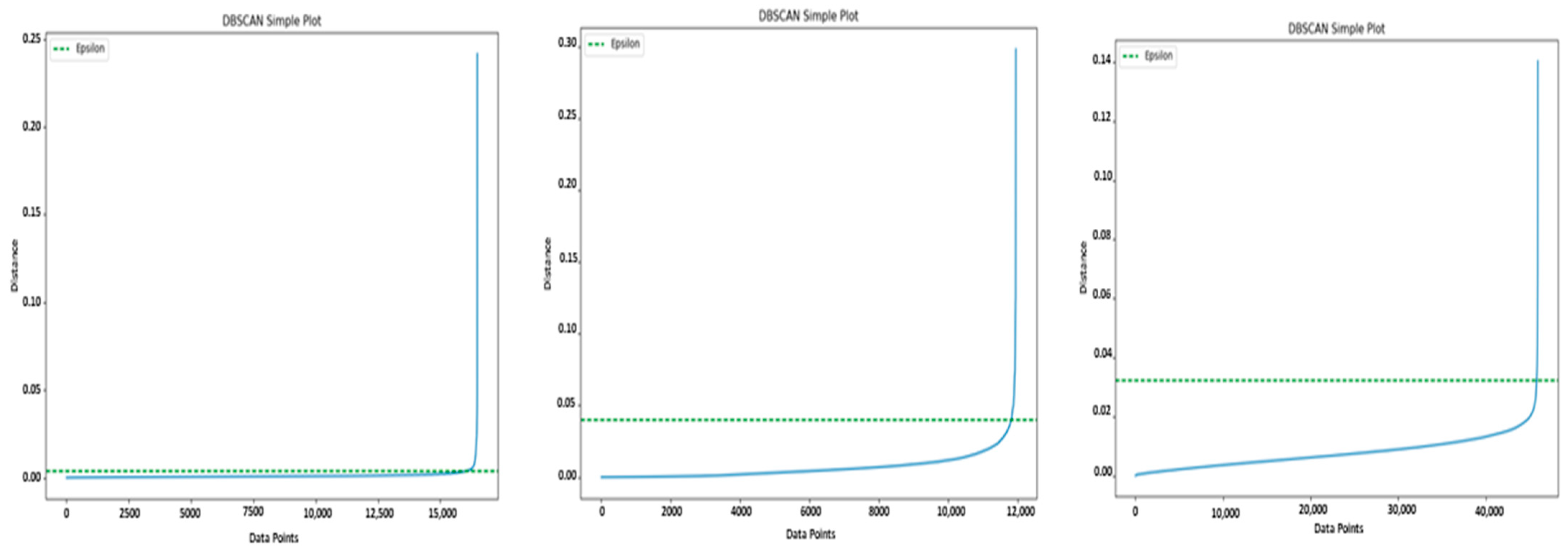
Figure 2 shows the data points of the graph, ordered by their distance to the fourth nearest neighbor and the corresponding $\mathsf{\epsilon }\text{-}\mathrm{v}\mathrm{a}\mathrm{l}\mathrm{u}\mathrm{e}\mathrm{s}$ calculated with our method. As described in [2], determining the ideal $\mathsf{\epsilon }\text{-}\mathrm{v}\mathrm{a}\mathrm{l}\mathrm{u}\mathrm{e}\mathrm{s}$ involves identifying the distance value at the point of curvature of the elbow within the plot. However, it is worth noting that the user usually sets this parameter to optimize the effectiveness of the DBSCAN algorithm. Our method introduces a novel approach that enables the automatic determination of an appropriate $\mathsf{\epsilon }\text{-}\mathrm{v}\mathrm{a}\mathrm{l}\mathrm{u}\mathrm{e}$ by identifying the point on the plot where a curvature occurs that indicates a meaningful change in the structure of the data density.

To demonstrate the superiority of DBSCAN in detecting anomalies, we used other clustering algorithms in the clustering step of our method. The aim of the experiment was to emphasize the importance of using DBSCAN within the proposed method, in comparison to alternative clustering techniques, especially K-means and OPTICS, in conjunction with the results of the embedding stage. The evaluation criteria used for comparison included precision, recall, the F1 score, and accuracy. The results, which are summarized in

Table 2. Comparison with other clustering methods.

Datasets	Metrics	K-Means	OPTICS	DBSCAN
Amazon	Precision	0.96	0.93	0.93
	Recall	0.72	0.60	0.96
	F1 score	0.82	0.73	0.95
	Accuracy	0.71	0.59	0.90
ACM	Precision	0.85	0.96	0.98
	Recall	0.12	0.79	0.85
	F1 score	0.21	0.87	0.91
	Accuracy	0.13	0.77	0.84
YelpChi	Precision	0.85	0.85	0.86
	Recall	0.99	0.59	0.89
	F1 score	0.92	0.70	0.87
	Accuracy	0.85	0.57	0.78

, provide information on the differences in performance between the various methods. In particular, the precision metric quantifies the proportion of correctly identified positive instances out of all predicted positive instances and indicates the model’s ability to avoid false-positive instances. Recall, on the other hand, measures the proportion of true positive instances correctly identified by the model and illustrates its ability to capture all relevant instances. The F1 score, which combines precision and recall, provides a balanced assessment of the overall effectiveness of the model. Finally, accuracy indicates the proportion of correctly classified instances in the entire dataset and provides a general overview of the model’s performance. The analysis of the results shows that the proposed method using DBSCAN, in conjunction with the embedding results, outperforms both K-means and OPTICS in all evaluation metrics. This superiority emphasizes the effectiveness of DBSCAN in accurately identifying clusters within the dataset, especially in scenarios where the clusters have different densities and irregular shapes. The robustness of DBSCAN in handling noise and effectively partitioning the dataset into different groups contributes to its superior performance compared to K-means and OPTICS.

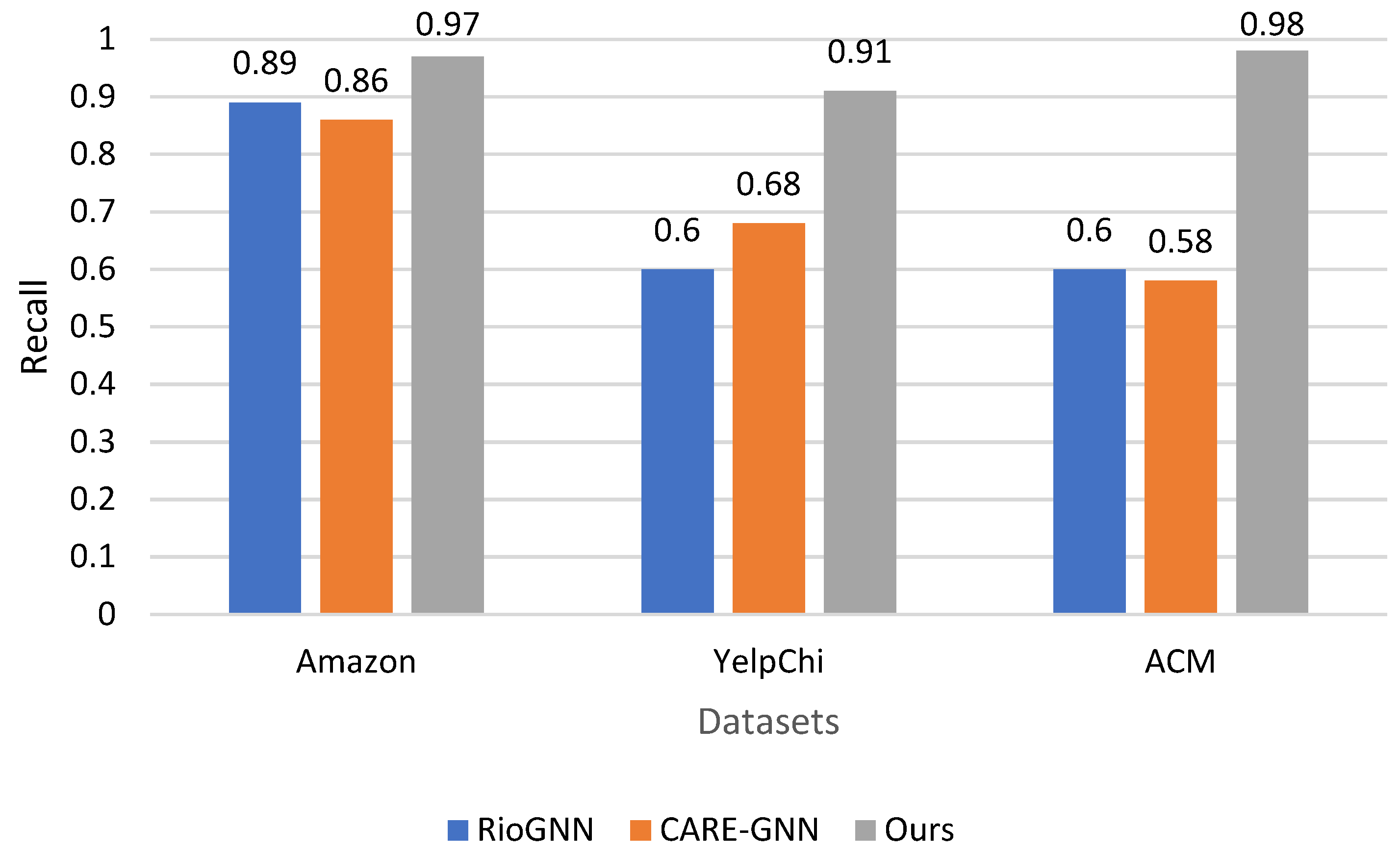
The primary metric used for evaluation is recall, which measures the proportion of true anomalies correctly identified by each method. As shown in Figure 3, our results are convincing evidence of the superiority of our method in detecting anomalies in all datasets. On the Amazon dataset, our method outperforms both RioGNN and CARE-GNN, with a recall of 0.97, compared to 0.89 and 0.86, respectively. On the YelpChi dataset, our method also shows a significantly higher detectability of 0.91, compared to 0.6 for RioGNN and 0.68 for CARE-GNN. This trend also continues in the ACM dataset, where our method achieves a recall of 0.98, exceeding the recall values of 0.6 for RioGNN and 0.58 for CARE-GNN.

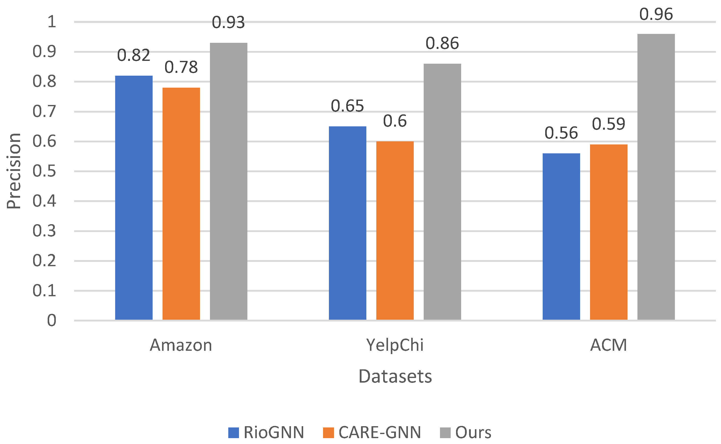
Precision is used as a secondary metric to quantify the accuracy of anomaly detection by measuring the proportion of correctly identified anomalies out of all instances labeled as anomalous. As can be seen in Figure 4, our investigation of the precision values shows a consistent trend where our method outperforms both RioGNN and CARE-GNN on all datasets. On the Amazon dataset, our method achieves a precision of 0.93, outperforming the precision values of 0.82 for RioGNN and 0.78 for CARE-GNN. A similar pattern can be observed in the YelpChi dataset, where our method has an accuracy of 0.86, outperforming RioGNN’s accuracy of 0.65 and CARE-GNN’s accuracy of 0.6. Furthermore, on the ACM dataset, our method outperforms the accuracy values of 0.56 for RioGNN and 0.59 for CARE-GNN, with an accuracy of 0.96. The superiority of our method in accuracy emphasizes its effectiveness in accurately identifying anomalies in different datasets. This higher precision is particularly beneficial in anomaly detection, where accurate identification of anomalies is of paramount importance for minimizing the number of false positives and ensuring the reliability of detected anomalies.

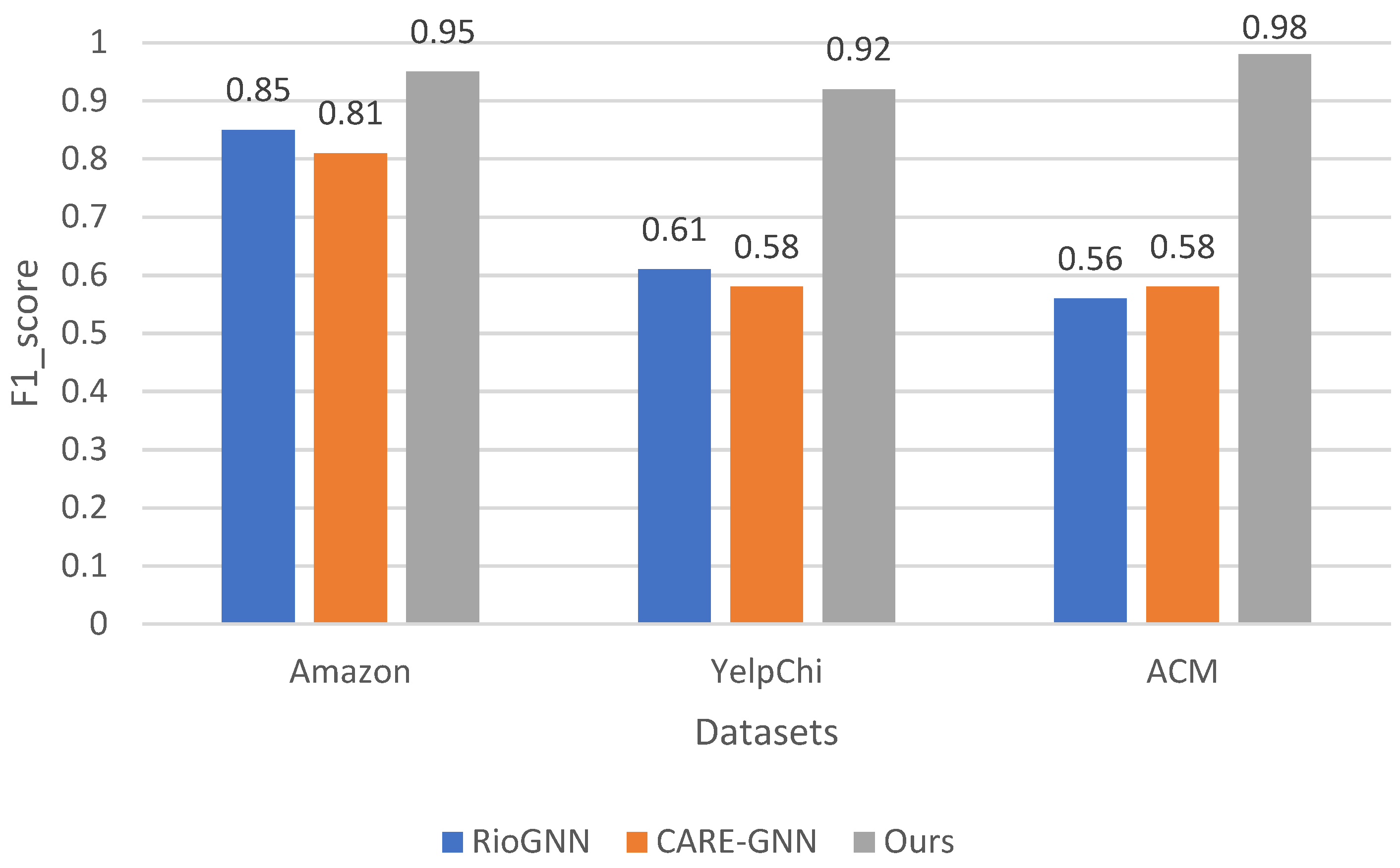
The third metric for performance evaluation is the F1 score, which provides a balanced measure of the precision and recognition value of a model. This is particularly valuable in anomaly detection, where the goal is to accurately identify anomalies while minimizing false positives and false negatives. As shown in Figure 5, when looking at the F1 score values, our method consistently outperforms both RioGNN and CARE-GNN in all datasets. On the Amazon dataset, our method achieves an F1 score of 0.95, outperforming the F1 scores of 0.85 for RioGNN and 0.81 for CARE-GNN. On the YelpChi dataset, our method also achieves a remarkable F1 score of 0.92, outperforming RioGNN’s F1 score of 0.61 and CARE-GNN’s F1 score of 0.58. On the ACM dataset, our method also outperforms RioGNN’s F1 score of 0.56 and CARE-GNN’s F1 score of 0.58 with an impressive F1 score of 0.98. The superiority of our method in terms of the F1 score underscores its effectiveness in achieving a balance between precision and recall, which is critical for accurate detection of abnormalities. By achieving higher F1 scores on different datasets, our method demonstrates its ability to reliably detect abnormalities while minimizing both false-positive and false-negative results.

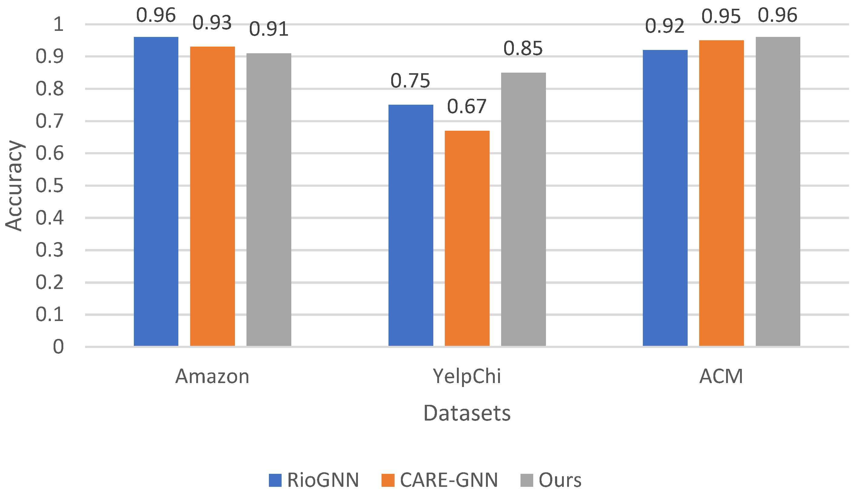
The final metric for performance evaluations is accuracy, which indicates the general correctness of the anomaly detection results. A look at the accuracy values in Figure 6 shows that our method consistently outperforms both RioGNN and CARE-GNN in all datasets. On the Amazon dataset, our method achieves an accuracy of 0.91, which is slightly lower than the accuracies of 0.96 for RioGNN and 0.93 for CARE-GNN. On the YelpChi dataset, our method also has a remarkable accuracy of 0.85, outperforming RioGNN’s accuracy of 0.75 and CARE-GNN’s accuracy of 0.67. Moreover, on the ACM dataset, our method outperforms RioGNN’s accuracy of 0.92 and CARE-GNN’s accuracy of 0.95, with an impressive accuracy of 0.96. The superiority of our method in terms of accuracy emphasizes its effectiveness in accurately detecting anomalies in different datasets. By consistently achieving higher accuracy scores, our method demonstrates its ability to accurately detect anomalies and correctly classify instances. Furthermore, the robust performance of our method across multiple datasets highlights its reliability and generalizability.

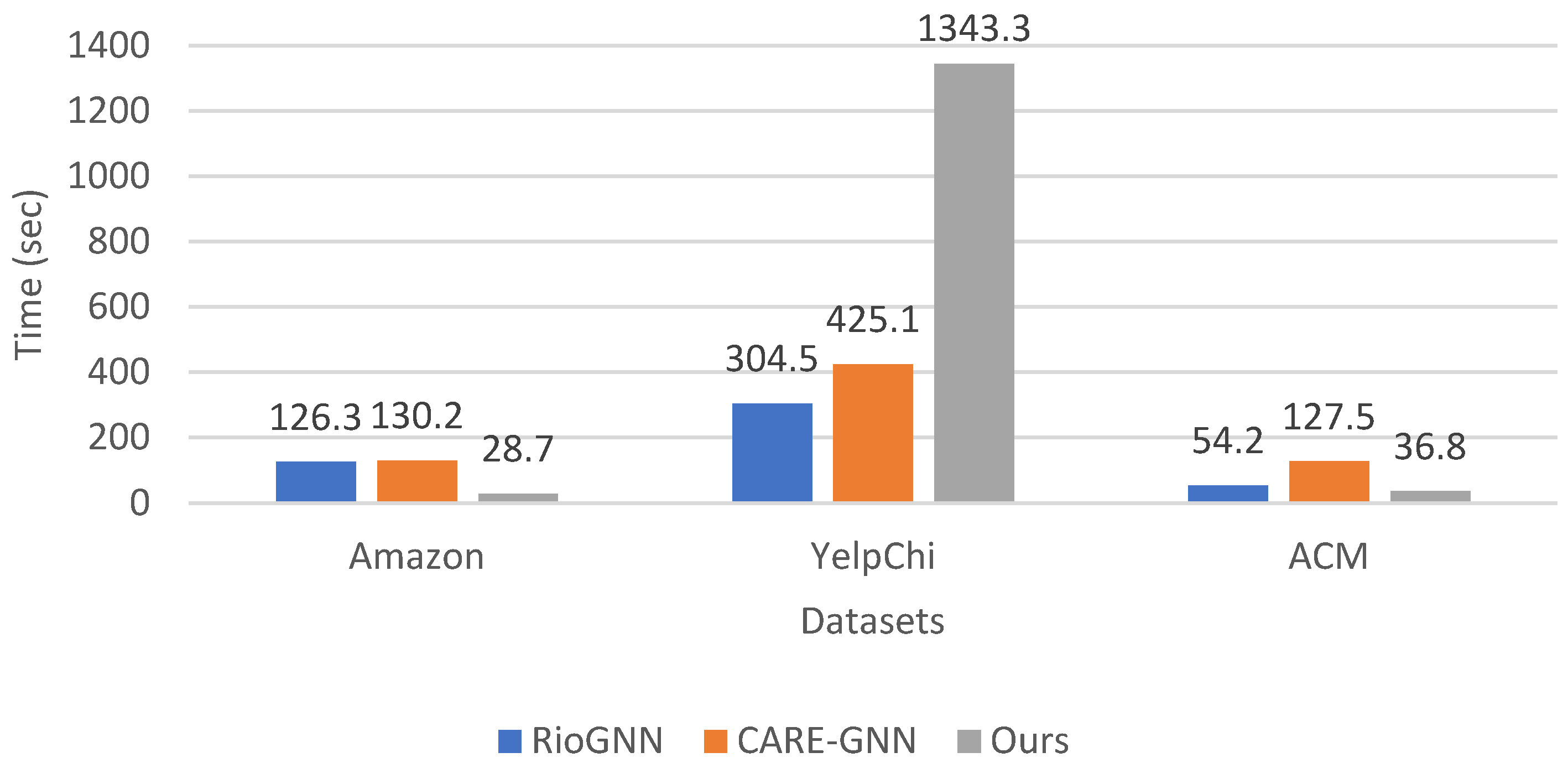
We analyzed the execution time of our proposed anomaly detection method compared to RioGNN and CARE-GNN on the datasets Amazon, YelpChi, and ACM. The execution time metric provides valuable insights into the computational efficiency of each method, which is a crucial factor in real-world applications. As illustrated in Figure 7, the re-evaluation of the execution time values shows that our method has a higher execution time compared to RioGNN and CARE-GNN, in some cases. For the Amazon dataset, our method has an execution time of 28.7 s, which is significantly lower than the execution times of 126.3 s for RioGNN and 130.2 s for CARE-GNN. For the ACM dataset, our method also outperforms the execution time of RioGNN (54.2 s) and CARE-GNN (127.5 s), with an execution time of 36.8 s. However, for the YelpChi dataset, the execution time of our method is 1343.3 s, which is significantly higher than the execution time of RioGNN (304.5 s) and CARE-GNN (425.1 s). This suggests that our method may not be as computationally intensive as the other methods in this scenario. However, it is important to note that a balance between computational efficiency and other performance metrics, such as accuracy and effectiveness should be considered when interpreting the execution time results. Even though our method has a higher execution time in some cases, it may still provide higher accuracy or other benefits that outweigh the longer computation time. In summary, while our method may have higher execution times in certain scenarios, its overall performance should be evaluated comprehensively, by considering multiple metrics and their respective trade-offs.

5. Conclusions

In this paper, we proposed an anomaly detection method based on Graph Convolutional Networks to learn discriminative node embedding and DBSCAN to distinguish abnormal nodes from normal nodes. We designed a neural network that learns features by inspecting neighboring nodes and exploited their structural information. In addition, we added a multivariate normal distribution component to represent our learned graph as latent two-dimensional data. To efficiently detect anomalies, we also developed an automated DBSCAN that computes a value of the hyper parameter epsilon based on the node embedding result and returns normal and abnormal clusters. The experiments conducted on three real-world benchmark datasets have shown that our method consistently outperforms state-of-the-art alternatives on all datasets. Furthermore, we have demonstrated the importance of DBSCAN compared to two other very popular clustering methods.

Despite the promising results of the proposed method in detecting anomalies in large graphs using GCNs and an automated method to determine the DBSCAN hyperparameter’s epsilon, some limitations need to be considered. First, the performance of GCNs strongly depends on the hyperparameter settings, such as the number of layers and the learning rate. This means that our study may not have explored the entire space of hyperparameters, which could limit the robustness of the results. Although we have automated the determination of epsilon, DBSCAN still requires another important parameter, namely the minimum number of points required to form a dense region ($\mathrm{m}\mathrm{i}\mathrm{n}\mathrm{P}\mathrm{t}\mathrm{s}$), which we have defined according to the recommendations of previous studies.

From a computational point of view, large graphs require significant computational resources for both GCN training and DBSCAN clustering. The scalability of our method might be limited by the available computational infrastructure. Moreover, the generalizability of our results to other domains and dynamic graphs is not guaranteed, as performance may vary, and additional adaptations may be required for evolving graphs.

Finally, the evaluation metrics used in this paper may not capture all aspects of anomaly detection effectiveness in different applications. Future work should consider additional metrics and case-specific developments to provide a more comprehensive evaluation. We also plan to further develop our method to adaptively detect anomalies on edges and subgraphs in dynamic network environments.