Article

N-Dimensional Non-Degenerate Chaos Based on Two-Parameter Gain with Application to Hash Function

School of Electronic Engineering, Heilongjiang University, Harbin 150080, China
*
Author to whom correspondence should be addressed.
Electronics 2024, 13(13), 2627; https://doi.org/10.3390/electronics13132627
Submission received: 2 May 2024 / Revised: 21 June 2024 / Accepted: 2 July 2024 / Published: 4 July 2024
(This article belongs to the Special Issue Nonlinear Circuits and Systems: Latest Advances and Prospects)

Abstract

:
The Lyapunov exponent serves as a measure of the average divergence or convergence between chaotic trajectories from the perspective of Lyapunov exponents (LEs). Chaotic systems with more and larger positive LEs have more complex dynamical behavior and can weaken the degeneration of digital chaos. Some existing control algorithms for chaos need more and larger preset parameters, which are not favorable for practical application; others require the original system to satisfy specific conditions, which lack generality. To address the deficiencies of these algorithms, this paper proposes a construction algorithm of N-dimensional discrete non-degenerate chaos based on two-parameter gain (ND-NCTG), which can realize the non-degenerate or non-chaotic control of chaotic systems by only two control parameters. We take a 3D chaotic system as an example and analyze the relationship between control parameters and LEs, as well as the characteristics of chaotic sequences, to verify the effectiveness and reliability of the algorithm. In addition, since the initial value sensitivity of the chaotic system coincides with the sensitivity in input information for the hash function, this paper takes the proposed chaotic construction algorithm as the basis to design a bidirectional diffusion chaotic hash function. The effectiveness and security of this hash algorithm are verified by sensitivity, statistical distribution and collision analysis. Compared with similar algorithms, both the non-degenerate chaotic construction algorithm and the hash function algorithm proposed in this paper have better performance and can meet the application requirements of secure communication.

1. Introduction

Over the past half-century, research on chaos has evolved from the study of phenomena [1,2,3] to theoretical and applied research [4,5]. Chaotic systems possess unique dynamic characteristics, including pseudo-randomness, ergodicity and sensitivity to initial conditions. Due to these properties, chaotic systems have been widely applied in fields of image encryption, chaos synchronization, weak signal detection and differential chaos shift keying [6,7,8,9].
Systems with excellent chaotic characteristics in the continuous domain may exhibit completely opposite behavior after implementation on finite-precision hardware. The reason for this is sensitivity to initial conditions in chaotic systems, ensuring that trajectories gradually diverge with even tiny differences. However, the truncation effect of finite precision causes the loss of tiny differences, resulting in the overlapping of initially distinct chaotic trajectories and the transition to periodic orbits, leading the system into a periodic state. This means that chaotic sequences under finite precision must be periodic [10], and their dynamical characteristics will deteriorate or even disappear. Additionally, Addabbo et al. [11] propose to increase the period of the Renyi map under finite precision by optimizing its mathematical model. With further research on chaotic theory [12,13,14], low-dimensional chaotic systems are susceptible to threats such as time-series prediction methods and phase space reconstruction algorithms due to their small key space and low complexity [15,16,17]. Traditional low-dimensional chaos can no longer meet the demands of secure communication.
The Lyapunov exponent serves as a numerical index used to measure the average level of convergence or divergence between chaotic trajectories. From the perspective of LEs, low-dimensional chaotic mappings or high-dimensional degenerate chaotic systems, the number of positive LEs cannot reach the theoretical maximum [18,19]. On the other hand, high-dimensional non-degenerate chaotic systems with more and larger positive LEs exhibit more complex structures and richer dynamical characteristics. Consequently, scholars have focused on the enhancement and control of high-dimensional chaos in recent years, proposing numerous efficient algorithms [20,21,22,23,24].
Among these excellent algorithms, some control algorithms require further improvement. The controlled matrices constructed in the literature [25] are strictly diagonally dominant matrices, and the special structure of this matrix leads to smaller off-diagonal elements compared to diagonal elements, causing the chaotic sequences to be mainly controlled by the diagonal elements. Wang et al. [26] use matrix similarity transformation to construct the coefficient matrix inversely, but numerical overflow issues arise in the matrix inversion operation. Fan et al. [27] utilize singular value decomposition (SVD) to avoid matrix inversion, yet it suffers from high computational complexity and the requirement of many preset parameters. Literature [28] is based on the upper triangular matrices approach, resulting in numerous zero elements in the coefficient matrix, thereby reducing the correlation between chaotic variables and weakening the chaotic properties. Similarly, Fan et al. [29,30] utilize the property of upper triangular matrices to achieve non-degenerate chaotic systems, where the highest-dimensional chaotic mapping degenerates into a Renyi map with poor chaotic characteristics. Additionally, Ding et al. [31] cascade and transform multiple chaotic mappings into upper triangular matrices, which suffers from the same drawbacks of the two aforementioned methods. He et al. [32] introduce a construction algorithm for continuous chaotic systems that requires the original coefficient matrix to be a nominal matrix and heavily relies on debugging parameters, lacking generality. The construction algorithm proposed in reference [33], based on Pascal matrices, lacks flexibility due to the fixed rules for constructing Pascal matrices and cannot achieve non-degeneration. Wang et al. [34] propose a control algorithm based on nonlinear autoregressive filter structures; since the chaotic sequence of the kth dimension is a time delay of the k + 1 th dimension, the sequences are almost identical to each other and the chaotic system is actually one-dimensional chaos. Hua et al. [35] iteratively expand block matrices to gradually obtain the desired dimensional coefficient matrix, which retains numerous zero elements due to the characteristics of the chunked upper or lower triangular matrix.
Therefore, we propose a construction algorithm of ND-NCTG, where parameter σ controls the coefficient matrix to meet the non-degenerate condition and parameter γ further adjusts the magnitude of positive LEs. Taking a 3D chaotic system as an example, we analyze the phase portrait, bifurcation diagram, sequence joint entropy, etc. The parameters for all comparison algorithms are set according to the original literature, and adjustments are made to ensure that the systems have the same level of LEs. The experimental results demonstrate that the algorithm proposed exhibits superior performance compared to similar studies and can meet the practical requirements of secure communication. Furthermore, this algorithm has no special restrictions on the original matrix and the constructed coefficient matrices are not special matrices, resulting in greater generality.
With the successful cracking of MD5 and SHA-1 [36,37], SHA-2, with a similar structure to SHA-1, also faces the risk of being cracked. In recent years, many scholars have worked on the hash function and have proposed some excellent hash algorithms, which have greater advantages in speed and security compared with traditional hash algorithms such as SHA-1 and SHA-2 [38,39,40]. Since the sensitivity to initial conditions of chaotic systems matches the sensitivity requirement of the hash function to the input information, chaotic systems have been used as a sponge function to absorb the information [41,42].
Consequently, we propose a new chaotic hash function algorithm based on ND-NCTG. To resist differential attacks, this algorithm employs a bidirectional diffusion mechanism to spread differential bits throughout the entire plaintext, making it difficult for attackers to correlate changes in hash codes with differences in the plaintext. Comprehensive experimental analyses are conducted on the constructed hash algorithm, including sensitivity analysis, collision analysis, statistical analysis and speed comparisons. The experimental results demonstrate that, compared to existing algorithms, this algorithm exhibits superior performance across various metrics, meeting practical application requirements.

2. Construction Algorithm

We consider a discrete linear chaotic model as shown in Equation (1) and conduct an in-depth analysis of such chaotic systems:
X ( n + 1 ) = A · X ( n ) m o d M ,
where M represents the modulus for the modulo function, the state variable is represented by a one-dimensional vector X ( n ) = [ x 1 ( n ) , x 2 ( n ) x N ( n ) ] T and A is an N × N coefficient matrix.
For chaotic systems only containing linear terms, the Jacobian matrix for the k-th iteration of the chaotic system equals the coefficient matrix A with only constant terms, i.e., J k = A , k = 1 , 2 L , obtain matrix Φ as Equation (2):
Φ = J 1 · J 2 J L = A L ,
where L represents the number of iterations for the chaotic mapping.
We adopt the eigenvalue-based method to calculate the LEs. Let the N eigenvalues of matrix Φ be λ 1 ( Φ ) , λ 2 ( Φ ) λ N ( Φ ) ; then, the formula for calculating the LEs is Equation (3):
L E k = l i m L 1 L · l n | λ k ( Φ ) | = l n | λ k | , k = 1 , 2 N ,
where λ k represents the k-th eigenvalue of matrix A.
To further control the eigenvalue λ k of the matrix and the Lyapunov exponent L E k of the chaotic system, according to the following theorem, we establish the relationship between LEs and control parameters σ , α in this paper:
Lemma 1
([43]). when multiplying matrix A by a coefficient α 1 > 0 and satisfying condition λ k 0 , the corresponding eigenvalue λ k will change by a factor of α 1 .
Lemma 2
([43]). when adding a scaled identity matrix σ 1 · E to matrix A, the corresponding eigenvalue will become λ k + σ 1 .
By combining Theorems 1 and 2, we set two control parameters γ and σ to address the requirement that eigenvalues of the original coefficient matrix A must satisfy condition λ k 0 . Firstly, we extract the Jacobi matrix A of the original system, calculate its minimum eigenvalue λ m i n and set matrix B = ( A + ( | λ k ( A ) + σ | ) · E ) / σ , σ > 0 to shift all eigenvalues of matrix A such that they satisfy condition λ k ( B ) > 1 . Then, we set C = B · e γ , γ > 0 to control the magnitude of LEs while ensuring that the controlled system satisfies the non-degenerate condition. In summary, the controlled coefficient matrix C and its eigenvalues are given by Equation (4):
C = ( | λ m i n ( A ) | · E + A + σ · E σ ) · e γ λ k = ( | λ m i n ( A ) | + A + σ σ ) · e γ ,
where E represents the identity matrix.
Using the matrix C to construct a non-degenerate chaotic system inversely, we determine the relationship between the Lyapunov exponent and the eigenvalues as L E k = l n ( ( | λ m i n | + λ k + σ ) / σ ) + γ . Since the eigenvalues are shifted and scaled, the LEs always satisfy the condition L E k > 0 ; below are specific details of the algorithm (Algorithm 1).
Algorithm 1 Construction Algorithm of Non-degenerate Chaotic System
Input: A = [ a i j ] N × N , X ( n ) = ( x 1 ( n ) , x 2 ( n ) x N ( n ) ) T , γ > 0 , M, σ > 0 ;
where A serves as the N × N Jacobi matrix, X ( n ) is the initial value of chaotic system,
γ and σ are using to obtain desired LEs, M is the modulus of modulo function.
Step 1: α = e x p ( γ ) , λ = e i g ( A ) ;
where e i g ( · ) is the function to obtain the eigvalues of matrix A.
Step 2: λ m i n = m i n ( λ ) ;
where the λ m i n is the minimum of λ .
Step 3: C = α · ( | λ m i n | · E + A + σ · E ) / σ ;
where the E is an identity matrix.
Output:the chaotic system X ( n + 1 ) = C · X ( n ) m o d M .
The above algorithm only uses two control parameters, γ and σ . It can reduce the number of control parameters while effectively controlling LEs, and does not require the original chaotic system to satisfy restrictive conditions, thus demonstrating greater universality.

3. Characteristic Testing of Chaotic System

3.1. The Relationship between LEs and Control Parameters γ , σ

Firstly, in order to analyze the role of the parameter γ in controlling the non-degeneracy of chaotic systems, we fix the parameter σ = 0.01 and calculate the relationship curve between the LEs and the parameter γ . Secondly, we also examine the relationship curve between the LEs and the parameter σ ; since the control parameter must satisfy the non-degenerate condition γ > 0 , we fix γ = 0.01 . The results are shown in Figure 1. The purple ‘*’ represents the LEs obtained using the matrix A as the chaotic coefficient matrix, where A refers to a randomly generated matrix or a coefficient matrix obtained by solving the Jacobi matrix of a discrete degenerate chaotic system that satisfies Equation (1), while the green ‘*’ represents the minimum LEs when the controlled system realizes non-degenerate conditions.
From Figure 1, it is evident that the relationship between LEs and parameter σ follows a decreasing trend in natural logarithmic form. Since ( λ k + | λ m i n | + σ ) / σ is always not less than 1, the minimum LEs of chaotic systems always satisfy the non-degenerate condition. Therefore, by configuring the control parameter σ , we can ensure that all LEs are greater than 0. Additionally, the LEs exhibit a linear growth relationship with the control parameter γ , indicating that γ can further adjust the magnitude of the Lyapunov exponent in the chaotic system. As a result, the control parameters γ and σ can effectively regulate the LEs, avoiding the situations where setting larger parameters results in smaller gains in LEs and mitigating the risk of numerical overflow.
The relationship between LEs and control parameters for the algorithm proposed in this paper is compared and analyzed with existing construction algorithms of chaos, as shown in Table 1.
From the table above, it is evident that the other algorithms proposed, except for method [44], have a number of control parameters related to the dimension of chaotic systems. Although the number of control parameters is lower, the algorithm proposed in [44] fails when the eigenvalue of the original systems equals 0. The algorithm proposed in this paper always only has two control parameters, which are independent of the dimension. This has some advantages over the existing non-degenerate chaotic construction algorithms in terms of effectiveness, number of parameters and universality.

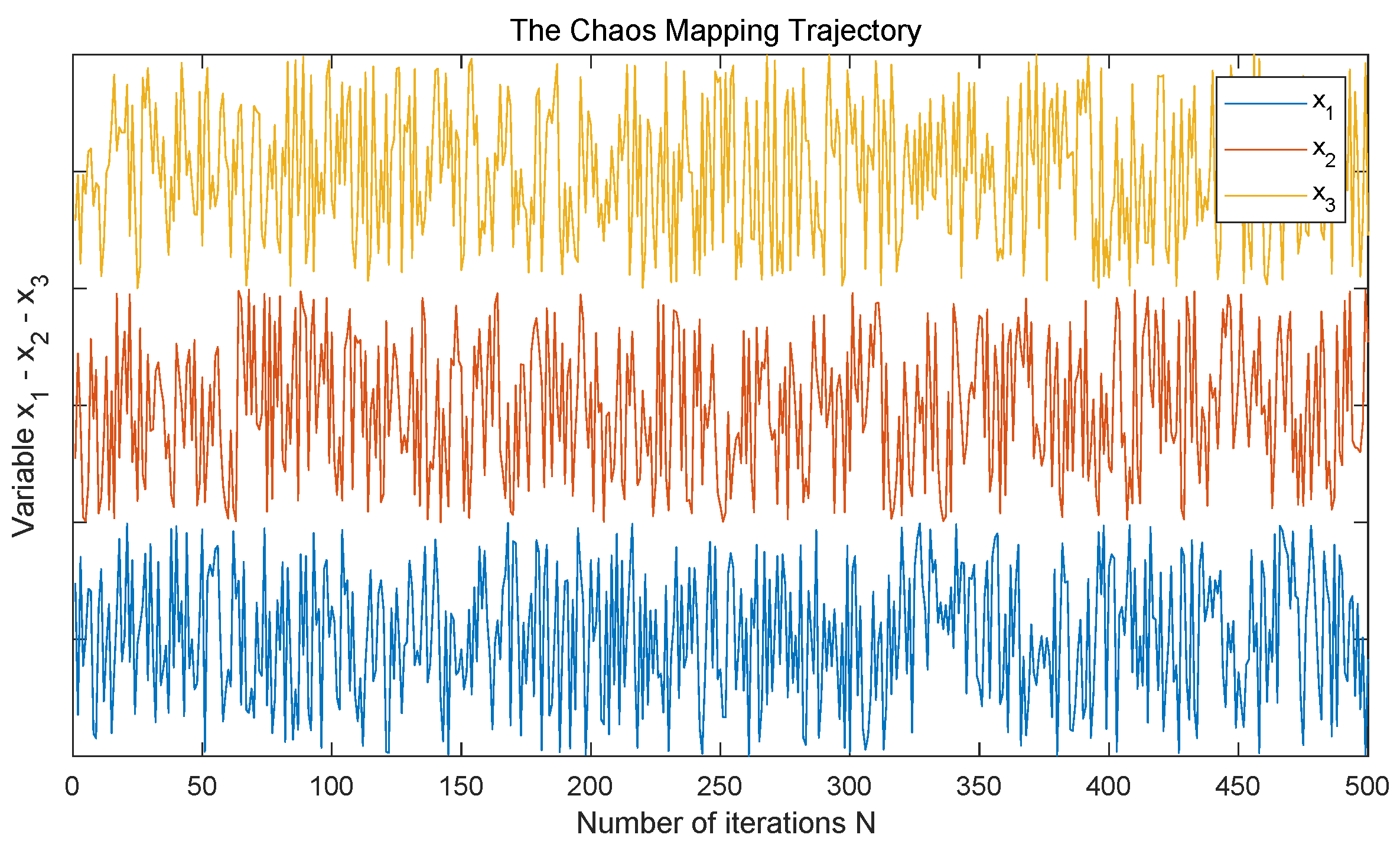
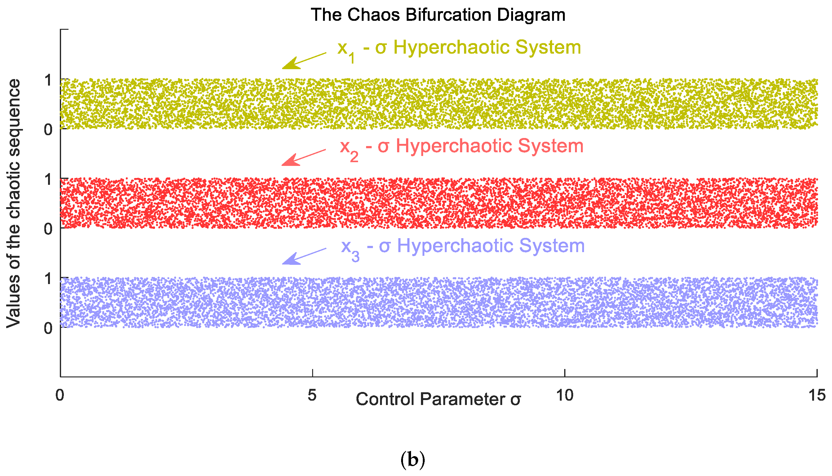
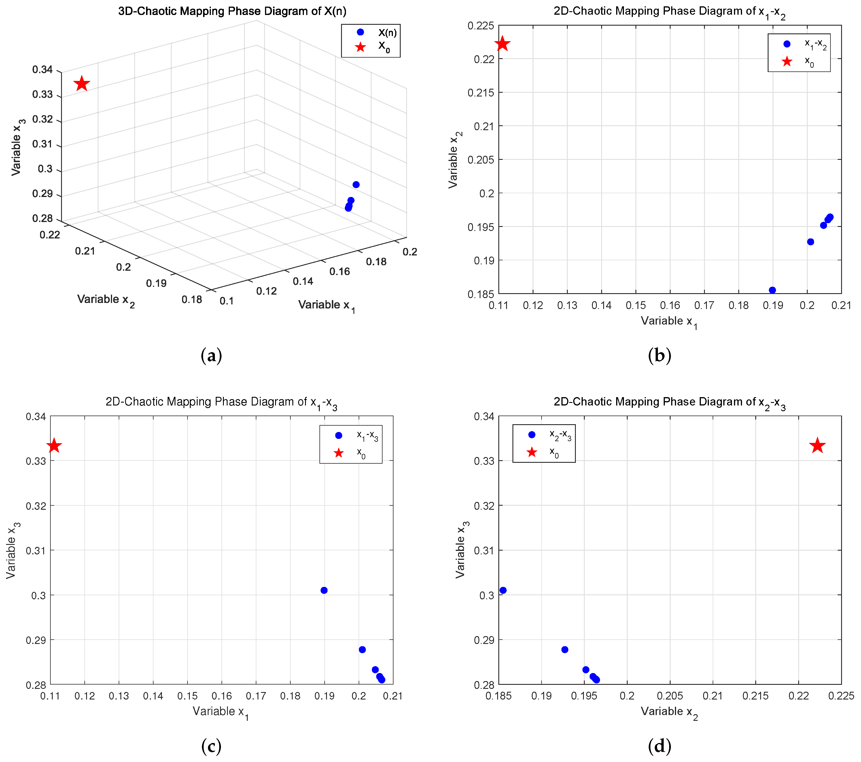
3.2. Chaotic Phase Diagrams and Bifurcation Diagrams

In order to verify the effectiveness of the proposed algorithm, a 3D non-degenerate chaotic system is constructed using a 3 × 3 matrix A generated randomly as an example, as shown in Equation (5):
A = 49 42 28 42 37 32 28 32 84 ,
using A as coefficient matrix of the chaotic system, its Lyapunov exponent is calculated as L E = [ 3.3269 , 3.7610 , 4.8440 ] T , and since there exists L E 1 < 0 , the original system is degenerate chaos. In order to realize chaos without degeneracy, the minimum eigenvalue of the coefficient matrix A is first calculated as λ m i n = 0.0359 . Then, the control parameters are set as γ = 2.1 , σ = 0.01 . According to the construction algorithm proposed, we obtain the controlled coefficient matrix C, as shown in Equation (6). To enhance clarity, matrix elements are shown to one decimal place.
C = 40 , 051.7 34 , 297.9 22 , 865.2 34 , 297.9 30 , 252.3 26 , 131.7 22 , 865.2 22 , 131.7 68 , 633.3 ,
We set the modulus coefficient as M = 1 and use the coefficient matrix C to construct the desired non-degenerate chaotic system inversely, as shown in Equation (7):
x 1 ( n + 1 ) = 40 , 051.7 · x 1 ( n ) + 34 , 297.9 · x 2 ( n ) + 22 , 865.2 · x 3 ( n ) m o d 1 x 2 ( n + 1 ) = 34 , 297.9 · x 1 ( n ) + 30 , 252.3 · x 2 ( n ) + 26 , 131.7 · x 3 ( n ) m o d 1 x 3 ( n + 1 ) = 22 , 865.2 · x 1 ( n ) + 22 , 131.7 · x 2 ( n ) + 68 , 633.3 · x 3 ( n ) m o d 1 ,
According to Equation (4), the LEs of this controlled chaotic system are calculated as L E = [ 4.2018 , 10.4673 , 11.5495 ] T . Since LEs of this chaotic system are all greater than 0, it is a non-degenerate chaotic map.
The phase diagram of chaos is an important tool for the study of chaotic phenomena in nonlinear systems and is used to analyze the system’s dynamical behavior, stability and complexity. In order to verify the properties of the constructed 3D non-degenerate chaotic system, we set the initial states as X 0 = [ 0.1111 , 0.2222 , 0.3333 ] T and the number of iterations to be L = 10,000. Using the generated chaotic sequence S e q , the phase diagrams are calculated as shown in Figure 2. From the chaotic phase diagrams, there is no obvious aggregation or chunking of discrete points in the phase space. The chaotic sequence can be uniformly dispersed throughout the phase space, indicating that the chaos has good ergodicity and randomness in all directions.
The chaotic trajectory map is another important tool in dynamical systems, and can directly show the trajectory of systems throughout the iteration process. We take the first 500 values of S e q and draw its chaotic trajectory map, as shown in Figure 3. From the map, the chaotic sequence has no obvious period, and its trajectory exhibits noise-like characteristics, indicating that it has good pseudo-randomness. Comparing the three trajectories of this chaotic system, it can be seen that, unlike the literature [34], there is no obvious similarity between the chaotic trajectories of different dimensions in this paper, and all the chaotic sequences generated are valid.
The bifurcation diagram is one of the characteristics of nonlinear systems, through which one can visualize the complex behaviors exhibited by chaotic systems with parameters. At the same time, it is possible to determine whether there is a periodic window in the system that leads to defects in the structure, weakening properties of dynamics, resulting in a risk of being cracked. From Figure 1, it can be seen that as the control parameter σ grows, the minimum LEs of the system are always greater than 0. Since there is no fixed range of values for σ and γ , we set σ , γ [ 0.01 , 15 ] as an example, and the bifurcation diagram for the remaining cases of σ , γ > 0 is no different from the sample range. We adjust the control parameter σ , γ separately and calculate the bifurcation diagrams; the results are shown in Figure 4. It shows that the chaotic bifurcation diagrams in all dimensions are dense scattering maps within the range of values for the control parameters. Since there is no obvious periodic window, the constructed chaotic system exhibits a high degree of complexity, good pseudo-randomness and low risk of being cracked.

3.3. Periodization of Chaotic Systems

We apply this algorithm to realize no chaos, transforming systems originally in chaotic states into periodic or fixed-point states, demonstrating the universality of our proposed algorithm. Based on Equation (4), we provide the condition for de-chaoticization, as shown in Equation (8):
γ l n ( σ / ( λ m a x + | λ m i n | + σ ) ) ,
where λ m a x is the largest eigenvalue of the coefficient matrix A and σ > 0 .
Similarly, taking the aforementioned matrix A as an example, its maximum eigenvalue is computed to be γ m a x = 126.9707 . We set the control parameter as σ = 0.01 . According to the non-chaotic condition, the maximum value of the control parameter is calculated to be λ m a x = 9.4495 . Setting the control parameter as γ = γ m a x , we use Equation (4) to compute the coefficient matrix C and construct the non-chaotic system inversely. Calculating its LEs using Equation (3), we obtain L E = [ 7.3477 , 1.0822 , 0 ] T . Since all LEs are not greater than 0, it indicates that this system is in a non-chaotic state. Keeping the initial state constant, we iterate the system to generate a discrete sequence with length L = 10,000, denoted as S e q . The phase diagrams of the discrete mapping are illustrated in Figure 5; it can be seen that the phase diagrams consist of only a finite number of discrete points, indicating that the system has a short-period characteristic. This validates the transformation of the system from a chaotic state to a periodic state, aligning with theoretical analysis.
In addition, in order to analyze the role played by the parameters γ in controlling the chaotic system to achieve being chaos-free, we fix the parameter σ and analyze the relationship between γ and LEs, as shown in Figure 6. The purple ‘*’ is LEs calculated from the original matrix A as a chaotic coefficients matrix, and the green ‘*’ is maximum LEs of the controlled system when the control parameters are satisfied γ l n ( σ / ( λ m a x + | λ m i n | + σ ) ) . From the results above, it can be seen that LEs show a linear relationship with the change in control parameter γ that is effective in achieving chaos-free systems.

3.4. Periodic Testing of Digital Chaotic System

When a chaotic system is implemented on hardware with limited precision, it is referred to as digital chaos. Due to precision limitations, there must be periods of digital chaos. However, systems with relatively good chaotic characteristics can resist this degradation to some extent, resulting in longer periods. Therefore, we transform the constructed chaotic system into digital chaos and use the chaotic cycle-finding algorithm (CCFA) [20] to find its cycles. Since chaotic sequences generated under different initial conditions and hardware precision settings may have different periodic lengths, we set 1000 sets of random initial values X 0 and 6 different precision levels Q, and iterate CCFA to search for the average period under different precision conditions. The periods of chaotic systems constructed by our algorithm are compared with those proposed by other researchers, as shown in Table 2.
From the table above, it can be seen that, compared with other construction algorithms, the chaotic system that we constructed exhibits longer digital periods. Implemented on hardware with limited precision, it can resist the degeneration of chaotic characteristics, promoting the practical applications of chaos in life.

3.5. Joint Entropy

The joint entropy (JE) of high-dimensional chaotic sequences can measure the uncertainty in the joint distribution among dimensions of a chaotic system. An N-dimensional chaotic system can generate N sets of different chaotic sequences. If the range of values for state variable values is evenly divided into I sub-intervals, then JE of the N sets of chaotic sequences can be calculated by Equation (9):
JE = k 1 I k 2 I k N I P ( b k 1 b k 2 b k N ) · l o g 2 P ( b k 1 b k 2 b k N ) ,
where P ( b k 1 b k 2 b k N ) represents the joint probability of the N states of the chaotic system taking values in I intervals. When the conditions P ( b k 1 b k 2 b k N ) = P ( b k 1 ) · P ( b k 2 ) P ( b k N ) and P ( b k 1 ) = P ( b k 2 ) P ( b k N ) = 1 / I are met, the probability of N states independently taking values and falling within I intervals is the same. JE reaches its theoretical maximum, which can be calculated by Equation (10). The larger the JE of the sequence, the fewer limiting factors that affect the values of N chaotic state variables. This allows for a more random selection of values within the range, resulting in a distribution of sequences across intervals that is closer to a uniform distribution.
JE m a x = N · l o g 2 ( I ) ,
To test the variation in JE with the division interval I, while fixing the dimension N = 3 , we randomly generated 100 sets of initial values for 3D chaotic mappings, and iterated to obtain chaotic sequences with length L = I 5 under different numbers of partition intervals I = { 3 , 5 , 7 , 9 , 11 } . For each set of sequences, we calculated the average joint entropy J E I . The results are shown in Table 3.
Additionally, we analyzed JE with the variation in the matrix dimension N while fixing the number of partition intervals as I = 3 . We randomly generated 100 sets of initial values for 3D chaotic mappings. Under different dimensions N = { 4 , 6 , 8 , 10 , 12 } , we iterated them to obtain chaotic sequences of length L = 3 N + 1 and calculated the average joint entropy J E N for each set of sequences. The results are shown in Table 4.
Based on the above results, compared to similar chaotic construction algorithms, the JE of the algorithm proposed in this paper is closer to the theoretical maxima of J E I and J E N . The chaotic variables of the system can take on values more randomly within their range, demonstrating a high degree of uncertainty and uniformity.

3.6. Standard Uniform Distribution Test

To test whether the distribution of generated chaotic sequences satisfies U(0 1), we conduct statistical tests on the chaotic mapping sequences with length N = 1 × 10 6 . Statistical characteristics include mean, median, variance, skewness, kurtosis, probability density function (PDF), cumulative distribution function (CDF) and histogram distribution. The histogram distribution divides the range of values for the three state variables into intervals S = { 10 , 100 , 1000 } and then performs statistical analysis. The test results are shown in Table 5 and Figure 7.
The test results of our system shown in Table 5 are very close to the ideal values, indicating statistical characteristics consistent with a standard uniform distribution U(0 1). As depicted in the figure above, the cumulative distribution function of the chaotic variable X ( n ) exhibits an approximately linear relationship, with a slope close to 1, meeting CDF = x , x [ 0 , 1 ] for a uniform distribution. Uniformity is further evidenced by nearly identical histogram values across all statistical subintervals, suggesting standard uniform distribution characteristics. Moreover, the PDF curve aligns with the probability density function of a uniform distribution. Chaotic sequences with uniform distribution properties demonstrate better performance in practical applications, such as pseudo-random number generators.

3.7. Sequence Sample Entropy

Sample entropy (SE) is commonly used to analyze the nonlinear dynamic properties by quantifying the complexity of time series through comparing the similarity between adjacent sub-sequences. SE involves two parameters: the pattern dimension m and the similarity tolerance threshold r. Compared with other nonlinear dynamic methods such as the Lyapunov exponent, information entropy and correlation dimension, SE exhibits better consistency, especially with sequences having higher SE. Changing the values of m and r also results in relatively higher sample entropy values. Therefore, we set parameter m = 2 , r = 0.2 , vary the two control parameters of the system, σ and γ , and plot the 3D SE against the changes in both parameters, as shown in Figure 8. The figures indicate that the SE of the proposed chaotic system remains relatively stable across the entire parameter space without significant fluctuations. This suggests that the SE of the chaotic sequence is robust to changes in the control parameters.
Furthermore, to analyze the influence of dimension N for the chaotic system on the SE, we construct chaotic systems with different dimensions N = { 2 , 3 15 } using our proposed algorithm and existing algorithms. Starting from 100 sets of random initial values, sequences with length L = 1 × 10 4 are generated iteratively, and the average SE of each set of sequences is calculated. The results are shown in Figure 9. The results clearly indicate that, across different dimensions, the chaotic systems proposed in this paper exhibit higher average sample entropy than the excellent research works of other scholars, indicating a higher complexity of the chaotic systems. Furthermore, compared to other algorithms, SE has no significant fluctuation with changes in the chaotic dimension, demonstrating strong robustness.

3.8. Correlation Dimension

The correlation dimension (CD) is an indicator used to describe the randomness and complexity in dynamical systems or time series. It quantifies the dimensional properties of a system in phase space. If a nonlinear system has positive attractors, it implies a larger correlation dimension, further indicating a higher singularity of the strange attractor. Comparing our algorithm with existing algorithms, in order to obtain stable results, each method randomly generates 100 sets of chaotic mapping sequences with a length L = 1 × 10 4 , and their average CD is calculated. The statistical results are shown in Table 6. The data in the table indicate that the chaotic systems constructed in this paper have a larger CD, implying the presence of more coupling relationships and interaction modes within them, as well as greater degrees of freedom, making the dynamical characteristics of chaotic systems more complex and rich. Consequently, the complexity of the sequences is higher.

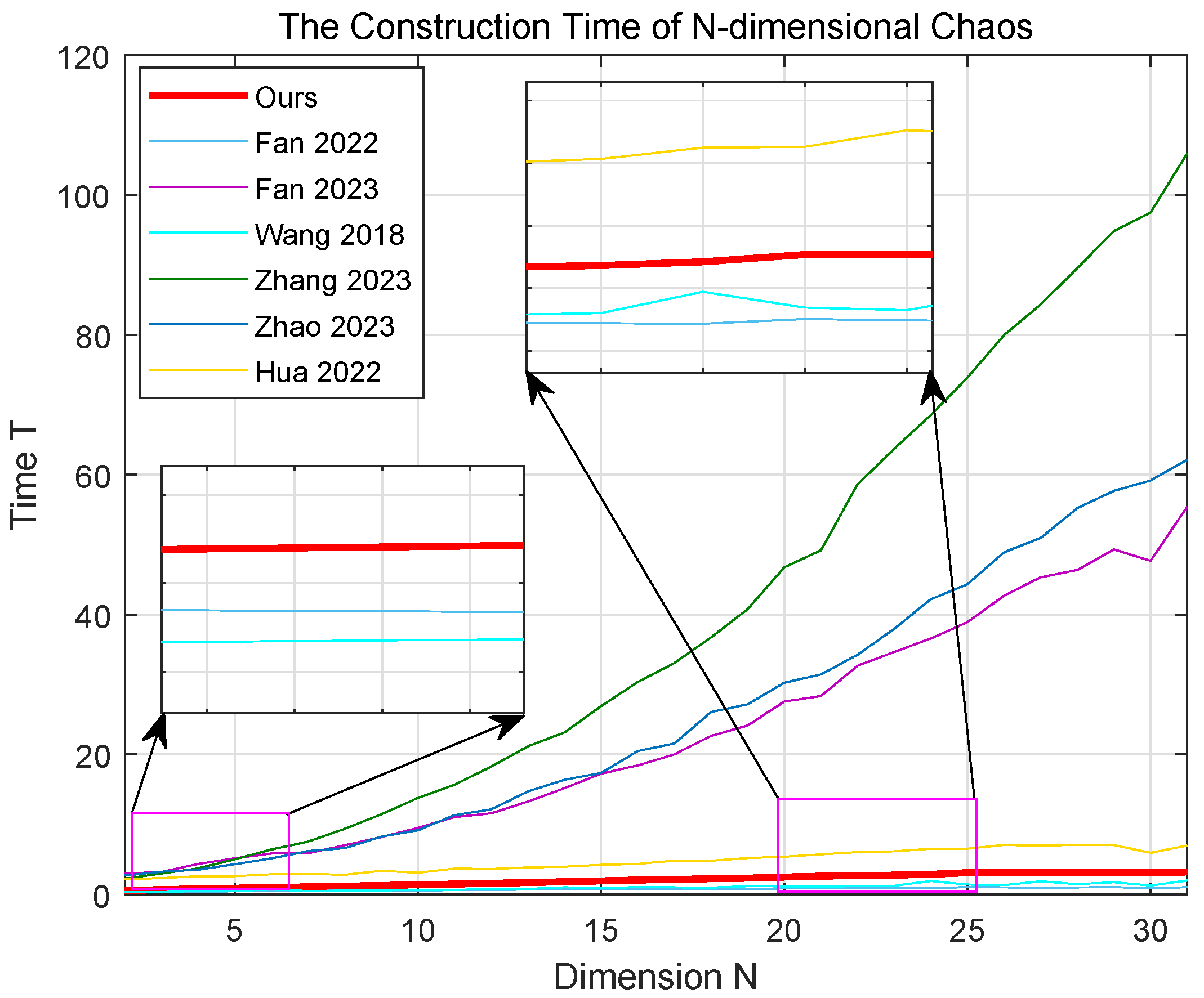
3.9. Time Complexity of Algorithms

The time complexity of an algorithm can measure whether a chaotic construction method is suitable for practical applications. To analyze the effectiveness of our algorithm proposed in practical applications, we select several similar construction algorithms. The algorithm complexity of the method proposed is compared with existing algorithms, and the results are shown in Table 7. It can be seen that the main complexity of our algorithm lies in the eigenvalue solving process, while the rest of the processes only involves simple matrix entity addtion and matrix entity multiplication. The algorithm complexity is relatively low and can meet the requirements in practical applications.
The time cost of an algorithm is not only related to its complexity but also to the types of operations and data involved. To evaluate the practical efficiency of the ND-NCTG algorithm, we run all N-dimensional chaotic generation algorithms 1 × 10 4 times, calculating their total time cost for N [ 2 , 31 ] . The results are shown in Figure 10. From the figure, it can be observed that, unlike the comparison results of algorithm complexity, the average time curve indicates that our algorithm has a faster construction speed compared to other algorithms in the case of low dimensions. As the dimension increases, the algorithm proposed in this paper can still construct chaotic systems at a relatively fast speed.

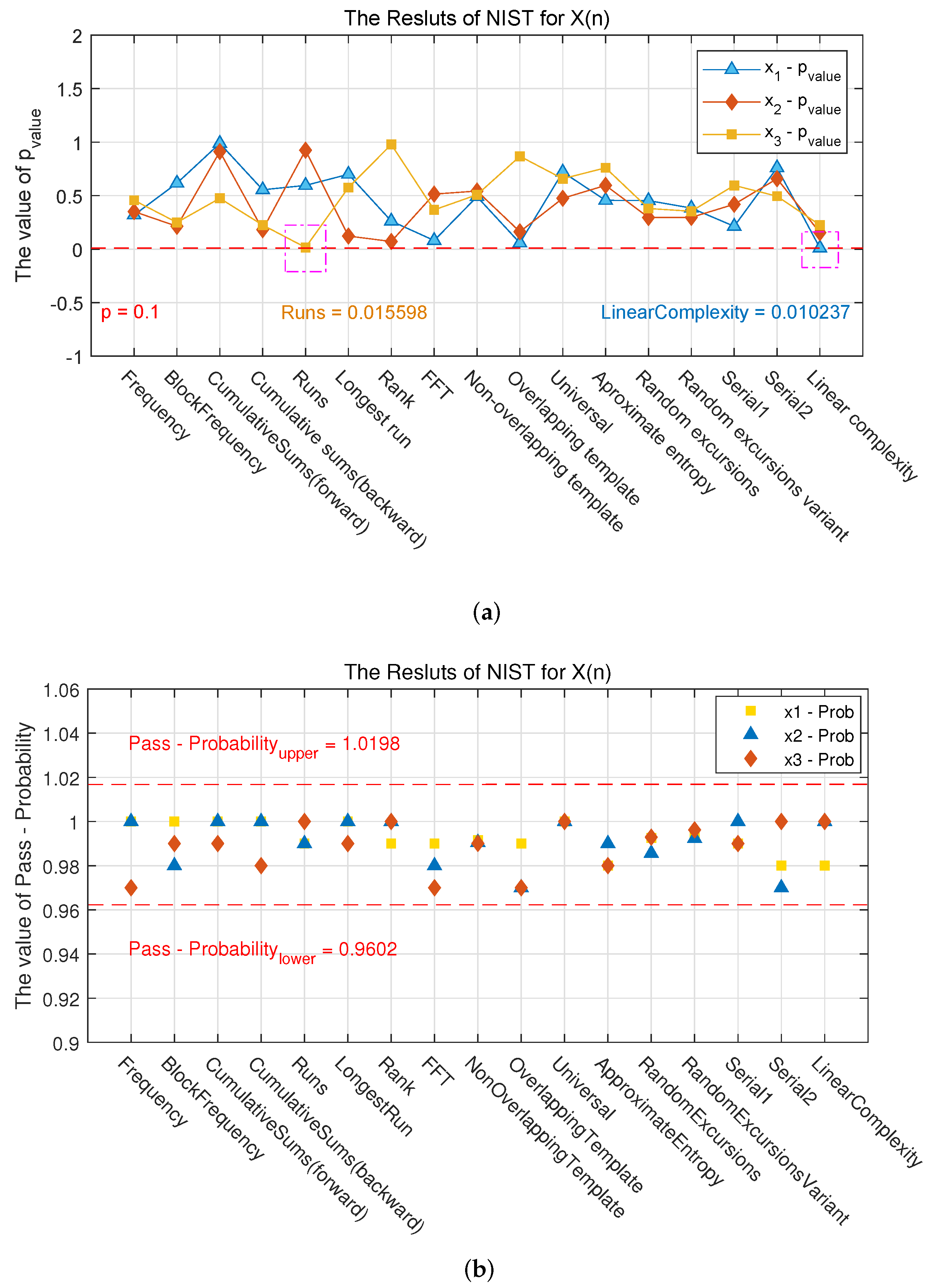
3.10. NIST SP800-22 Testing

In this section, we employ a shift-round quantization method to quantize discrete chaotic sequences [29], generating chaotic binary sequences for NIST testing. The system proposed in this paper is a high-dimensional discrete chaotic system, which differs from Renyi map in terms of chaotic structure and characteristics. Under finite precision conditions, it is distinct from PRNG implemented by the linear congruential generator [47]. The definition of shift-round quantization is given by Equation (11):
s k ( n ) = { f l o o r ( x k ( n ) m ) } 2 , n { 1 , 2 L } ,
where f l o o r ( · ) denotes the floor function, ≪ denotes the left shift operation, m represents the bit shift amount and s k ( n ) denotes the quantized sequence. Each chaotic sequence is quantized to generate a m-bit binary sequence. Then, we perform NIST tests on binary sequences; sub-test items output the confidence level p of passing the test, where, if p 0.01 , the hypothesis is accepted. When all p 0.01 and the pass probability P r o b fall within the interval [ 0.9602 , 1.0198 ] , it indicates that the generated binary sequence exhibits good statistical characteristics. Chaotic sequences S e q are converted into binary sequences and subjected to NIST random testing, and the NIST test results are shown in Figure 11. From the figure, it is observed that the pseudo-random numbers generated from the chaotic sequences have passed all the sub-test items of the NIST test suite. The binary sequences exhibit strong randomness, indicating that this chaotic system can meet the requirements for randomness in practical applications.

4. Hash Functions Based on Non-Degenerate Chaotic System

The algorithms proposed in this paper are implemented on the MATLAB R2019a software platform, running on a computer with an Intel i5-12400f CPU and 16 GB RAM. In this section, we will integrate the chaotic construction methods to propose a new hash function algorithm and analyze its performance.

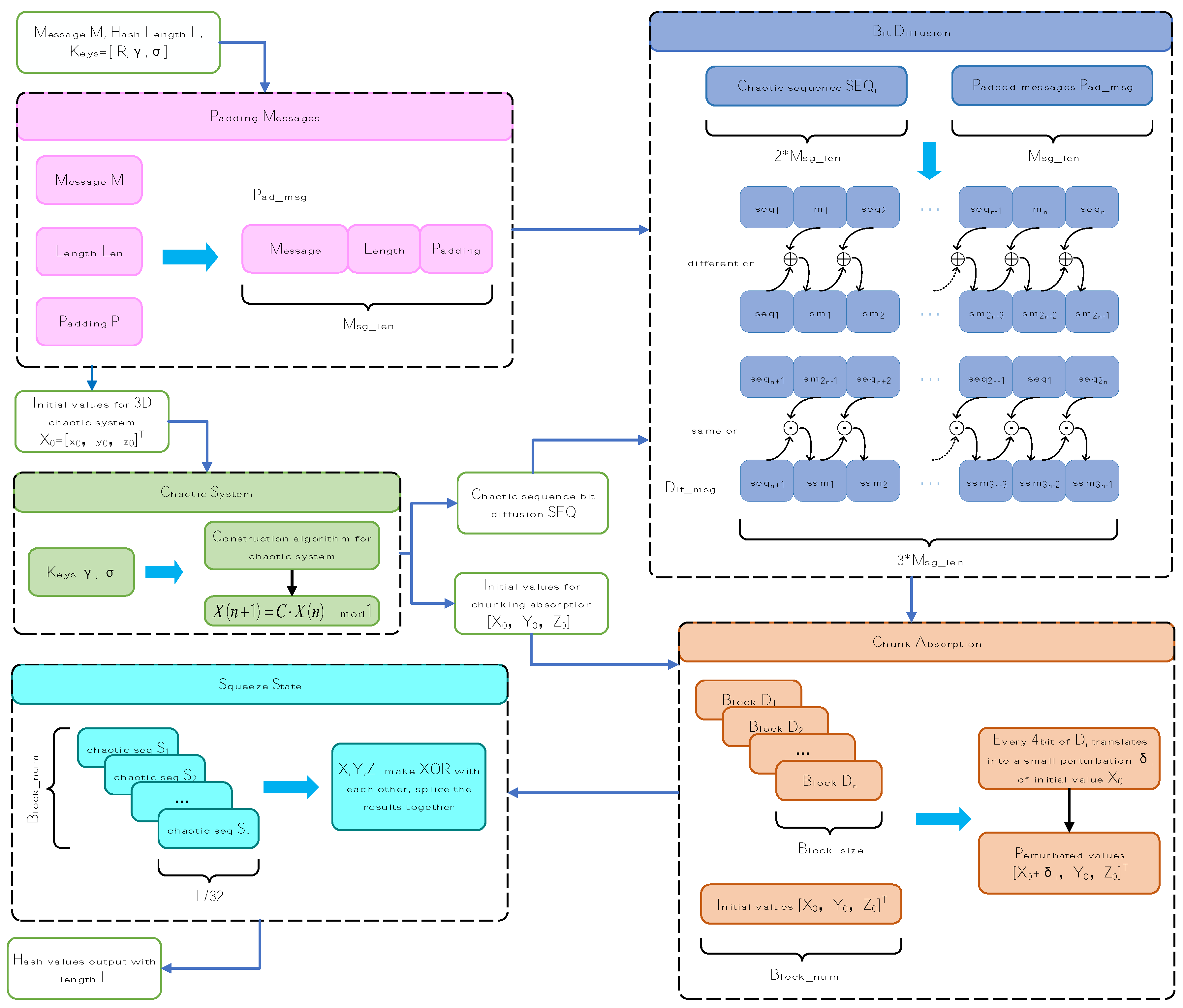
4.1. Hash Function Construction Algorithm

In response to the problems existing in existing chaotic-based hash functions, we introduce high-dimensional non-degenerate chaotic systems into the construction algorithm to address the issues of low-dimensional chaos while increasing the complexity of the hash algorithm. In order to design chaotic-based hash functions with improved properties, we follow the following recommendations [48]:
  • Include the length of messages in the padding to resist length extension attacks;
  • Significantly increase the number of iterations of the compression function to increase the difficulty of cryptanalysis;
  • Adopt mature structures in the design of the compression function to avoid security risks;
  • Ensure rapid diffusion of input differentials in algorithm design to resist arithmetic differential analysis methods.
Incorporating the above suggestions, we append the length information to the end of the plaintext message. Additionally, we design a bidirectional bit diffusion mechanism to rapidly spread differential bits throughout the entire message. We adopt the sponge function structure for absorbing and compressing information. The iteration rounds R and chaos control parameters γ , σ are used as keys, and we control the hash function using k e y s and hash length L, ultimately outputting a hash value with length L. The implementation block diagram for the proposed hash algorithm H a s h ( M , L , k e y s ) in this paper is shown in Figure 12.
Step 1: converting the input message M into binary bits and appending the length information L e n to the end, resulting in the extended message M . If the message M does not meet m o d ( M , B l o c k _ s i z e ) = 0 , it is padded with 0 bits to obtain the padded message P a d _ m s g with a length of M s g _ l e n .
Step 2: utilizing Equation (12), the length M s g _ l e n of the padded message is used as input to compute m s g _ v a l u e ; additionally, the first 24 bits of m s g _ v a l u e are separately used to generate x , y , z , obtaining the initial values [ x 0 , y 0 , z 0 ] T = [ x , y , z ] T / 255 of the chaotic system within the range of [ 0 , 1 ] :
m s g _ v a l u e = 1 + s i n ( 1 / 3.999 ( 1 / M s g _ l e n ) ( 1 + 1 / ( M s g _ l e n + σ 1 ) ) ) ,
where we set the parameter as σ 1 = 0.001 .
Step 3: utilizing the input keys γ and σ to construct the required 3D non-degenerate chaotic system. Iterating the chaotic system N = 9 M s g _ l e n / B l o c k _ s i z e times to obtain the chaotic sequence S e q . Dividing the sequence Z of S e q into 3 M s g _ l e n / B l o c k _ s i z e sets for the initial values [ X 0 , Y 0 , Z 0 ] T of the chaotic absorption stage. The sequences X and Y are taken from the end to the front to extract the first 8 bits of the sequence values with length M s g _ l e n / 8 , which are then combined into a binary sequence S E Q i . Utilizing S E Q i for forward XOR diffusion and backward XNOR diffusion to obtain the final binary diffusion sequence D i f _ m s g , with a length of 3 M s g _ l e n .
Step 4: the diffusion sequence D i f _ m a g is divided into B l o c k _ s i z e sub-sequences based on the block length B l o c k _ n u m . The sub-sequences are partitioned into 4-bit regions, where the 4 bits in odd regions are converted to δ i ( X ) and the 4 bits in even regions are converted to δ i ( Y ) . The initial values X 0 and Y 0 of the chaos are perturbed according to the following Equation (13):
X 0 ( n + 1 ) = X 0 ( n ) + δ n ( X ) Y 0 ( n + 1 ) = Y 0 ( n ) + δ n ( Y ) ,
where X 0 ( n + 1 ) and Y 0 ( n + 1 ) represent the initial values for the next iteration. After perturbing the chaotic state through iteration, the final state [ X n , Y n , Z n ] T is taken as the initial value for generating the absorption phase chaos. After N = R + L iterations, a chaotic sequence of length L / 32 is taken from the end, and the first 32 bits of the sequence values are extracted and converted into a binary sequence S i .
Step 5: the three sets of sequences in S i make XOR with each other to obtain the sequence X O R _ S i . Then, XOR operations are performed between B l o c k _ n u m sub-sequences to obtain the final hash value as Equation (14).
X O R _ S i = x o r ( x o r ( X i , Y i ) , Z i ) H a s h i = x o r ( X O R _ S i , H a s h i 1 ) ,
For subsequent experimental analysis, we use the aforementioned hash algorithm to compute hash values, with the hash length sets to L { 32 , 64 , 128 , 160 , 256 , 512 , 1024 } and each experiment repeated N { 256 , 512 , 1024 , 2048 , 10 , 000 } times. For each experiment, a randomly generated message M of length L e n = 50 × L is computed to obtain the corresponding original hash value H. Then, 1 bit is randomly selected from M for modification, resulting in a new hash value H l , n . This process is repeated N times for each experiment.

4.2. The Key Space of Algorithm

In encryption systems, the key space needs to be greater than 2 128 to avoid the possibility of brute-force attacks. Our system has three types of keys: the control parameters γ , σ and the iteration rounds R. The chaotic system is sensitive to small variations in the control parameters. Since the control parameters of this chaotic system do not have a fixed range, for ease of analysis, we fix γ ( 0 , 16 ] and σ ( 0 , 1 ] . Assuming that the precision is 1 × 10 14 for all values, the range of iteration rounds can be taken as R [ 1 , 10 14 ] , The total key space of the entire hash function is approximately 2 50 + 46 + 46 = 2 142 . At this point, the key space already satisfies the condition for resistance against brute-force attacks. However, since the chaotic control parameters do not have a fixed range of values, the actual key space of the hash function will be even larger, making it capable of resisting more powerful brute-force attacks.

4.3. Hash Sensitivity Analysis

In this subsection, we evaluate the sensitivity of the proposed hash algorithm to small changes in input messages. We make alterations to both the input message M and the key k e y s , calculate the hash value H of the original message and hash value C l , n of messages changed for different conditions and compute the Hamming distance between H and C l , n .
The six types of changes named C 1 C 6 are shown in Table 8. Specifically, C 1 replaces the first letter ‘T’ of the original message with ‘t’; C 2 replaces the symbol ‘a’ in the word ‘ c h a o t i c ’ with the symbol ‘e’; C 3 replaces the symbol ‘.’ at the end of the original message M with ‘,’; C 4 adds a space ‘’ at the end of the original message; C 5 introduces a slight modification to γ by altering γ = γ + 0.001 ; and C 6 introduces a slight modification to σ by altering σ = σ + 0.001 .
We set the hash lengths to L = { 32 , 64 , 128 , 160 , 256 , 512 , 1024 } , and the keys are set to [ γ , σ ] = [ 2.1 , 0.01 ] . The results of the hash value calculated are shown in Table 8. Additionally, the Hamming distances of all hash values are calculated, as shown in Figure 13. From the figure, it is evident that the Hamming distance HD between the computed hash values H l , n and the original hash values H, for slight modifications in the original message M and the k e y s , fluctuates slightly around the ideal value curve L / 2 .

4.4. Statistical Analysis of Scrambling and Diffusion

Scrambling and diffusion are two crucial operations in hash function design. Regarding the diffusion operation, ideally, modifying 1 bit of the input information should result in a 50 % change in the output hash bit. Meanwhile, scrambling operations create a complex relationship between input and output. In this subsection, statistical tests are conducted on the scrambling and diffusion operations in the hash function. By calculating the Hamming distance B l , n between H and H l , n , we plot the distribution histogram of B l , n , as shown in Figure 14.
In addition, for each set of experiments according to the hash length L and the number of repetitions N, the following statistical test items for B l , n are calculated.
  • The minimum number of changed bits as Equation (15);
    B m i n = m i n ( B i )
  • The maximum number of changed bits as Equation (16);
    B m a x = m a x ( B i )
  • The average number of changed bits as Equation (17);
    B ¯ = 1 N i = 1 N B i
  • The average rate of changed bits as Equation (18);
    P = B ¯ L × 100 %
  • The standard deviation of changed bits as Equation (19);
    Δ B = 1 N 1 i = 1 N ( B i B ¯ ) 2
  • The average rate of change in standard deviation as Equation (20).
    Δ P = 1 N 1 i = 1 N ( B i L P ) 2 × 100 %
The statistical test results obtained from the above equations are shown in Table 9. From the table, it is evident that the average changed bits B ¯ is close to the expected value L / 2 . By observing the average rate of changed bits P in different hash lengths L and iteration counts N, it can be noted that P is close to the ideal value of 50%. Therefore, the hash values generated by this algorithm result in an excellent performance in statistical tests for scrambling and diffusion. The small standard deviations of both the changed bits and the average rate of changed bits indicate the stability of the statistical results mentioned.

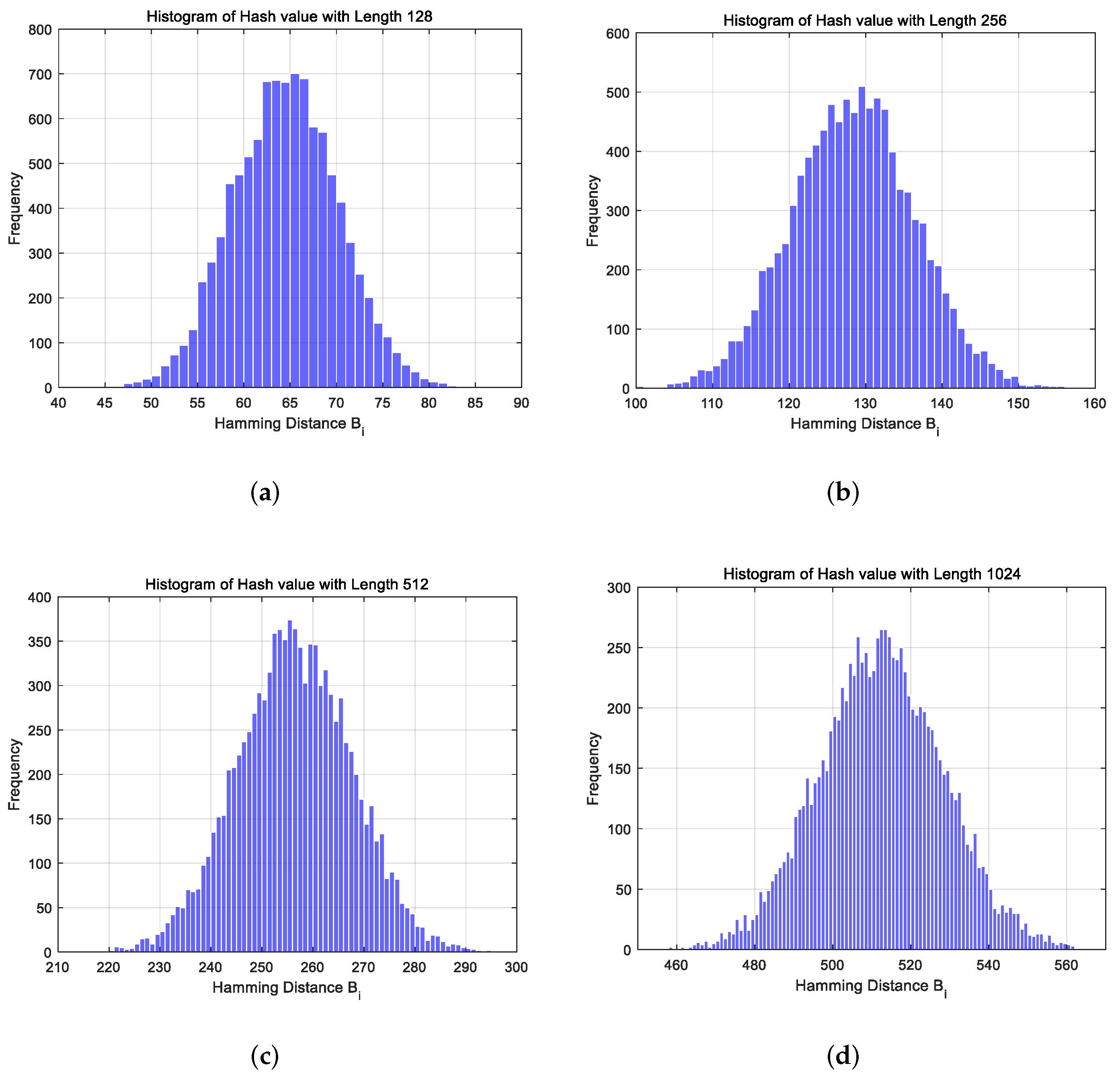
4.5. Uniform Distribution Analysis of Hash Values

The uniform distribution of hash values is directly related to the security of the hash function. This implies that the hash value must be uniformly distributed, and the probability of each bit taking the value of 0 or 1 is equally close to 50%. To achieve this, we count the number of hash values H where the corresponding bit is different from H l , n and count the maximum value M a x , minimum value M i n , mean M e a n and standard deviation S t d . The results are shown in Table 10.
The χ 2 test can verify the uniformity of sequence distribution. Therefore, for different hash lengths L and repetition counts N, we calculate the χ 2 value of the hash value using Equation (21):
χ 2 = k = 1 n ( O k E k ) 2 E k ,
where the observation O k is H l , n , corresponding to the case of length L and number of times N. The expected value E k = L / 2 and the significant level of the χ 2 test is set as α = 0.05 , and the statistical results are shown in Figure 15. The figure observes that the calculation results clearly satisfy χ 2 < χ α = 0.05 2 , indicating that the algorithm proposed in this paper has successfully passed the test and that the calculated hash value conforms to the uniform distribution.

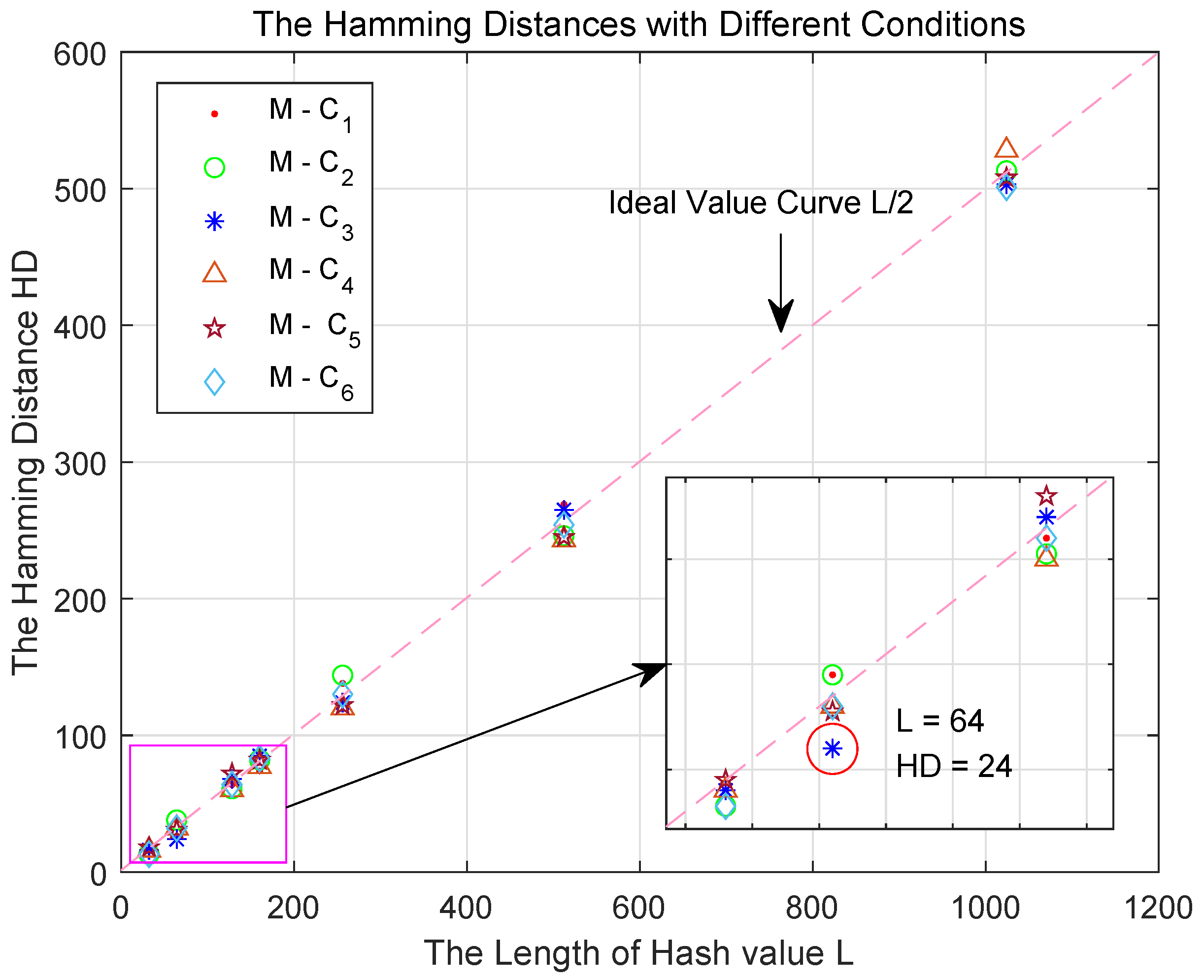
4.6. Collision Analysis of the Hash Function

A collision occurs when different messages M 1 and M 2 are computed to obtain the same hash value, and if it is difficult to find the pair of different plaintext, which means that the proposed algorithm is a robust hash function. In order to perform collision analysis, H l , n and H are converted into ASCII format (8 bits for each character) to obtain E l , n and E. Equation (22) is used to calculate the absolute difference between two hash values. The values e i and e i denote the ith ASCII character of two hash values, and the function d e c ( · ) maps the ASCII characters to the corresponding integer values.
d = i = 1 l e n / 8 | d e c ( e i ) d e c ( e i ) | ,
We calculate the absolute difference in H and H l , n , the maximum value M a x , the minimum value M i n , the average value M e a n and the average absolute difference in each character P c = M e a n / L ; the ideal value of P c is 85.3333, and the results are shown in Table 11. From the table, it can be seen that the absolute difference grows with the growth in hash length L; the average of the absolute difference for each character P c shows that the pattern of change for absolute difference under different hash lengths L is consistent.
If a character in the hash value H matches the corresponding character in H l , n , it is termed as a hit. We calculate the hit rate of hash values for different hash lengths L and numbers of experiments N and compare them with the ideal values [38], as shown in Table 12. From the table, the hit rate is very close to the ideal value under different conditions, indicating that the hash function has good anti-collision properties.

4.7. Comparative Analysis of Hash Performance and Speed

In this section, we compare the security and efficiency of the hash algorithm proposed with other similar works by means of statistical analyses of disruption and diffusion as well as speed, where the results of the statistical analyses are shown in Table 13. Hash function speed is an important indicator; for this reason, we generate messages with different lengths L e n , calculate the corresponding hash value, record the time spent and repeat N = 10,000 times to obtain the average computation time and compare with other types of hash functions; the results are shown in Figure 16. From the figure, it can be seen that the chaotic hash function proposed has a shorter computation time and can satisfy more practical applications.

5. Conclusions

The combination of a chaotic system and hash function promotes the development of the hash function on the one hand and extends the application scene of chaotic theory on the other hand. In this paper, an N-dimensional discrete non-degenerate chaotic system construction method based on two-parameter gain is proposed. The method is used to construct a 3D chaotic system as an example, which is analyzed from various perspectives, and the results show that the chaotic system has excellent properties. In addition, the chaotic system is used to construct an efficient keyed hash function algorithm that is capable of generating hash codes from 32 bits to 2048 bits. The security and effectiveness of the algorithm are experimentally proved through standard tests such as statistical analysis, collision analysis, key space analysis and comparative analysis. The key space of the algorithm is much larger than 2 234 , and thus it is considered to be a secure and fast algorithm. In our future work, we will apply this hash algorithm to more secure communication scenarios, including image, audio and video encryption.

Author Contributions

Conceptualization, X.D., X.W., H.H. and E.W.; methodology, X.D.; software, X.D.; validation, X.D., E.W. and X.W.; investigation, H.H. and E.W.; writing—original draft preparation, X.D.; writing—review and editing, X.D. All authors have read and agreed to the published version of the manuscript.

Funding

This research was funded by Heilongjiang Natural Science Foundation (No. JJ2019LH1317).

Informed Consent Statement

Not applicable.

Data Availability Statement

The data can be shared up on request.

Conflicts of Interest

The authors declare no conflicts of interest.

References

  1. Din, Q.; Naseem, R.; Shabbi, M. Predator-Prey Interaction with Fear Effects: Stability, Bifurcation and Two-Parameter Analysis Incorporating Complex and Fractal Behavior. Fractal Fract. 2024, 8, 221. [Google Scholar] [CrossRef]
  2. Pacheco, P.; Mera, E.; Navarro, G.; Parodi, C. Urban Meteorology, Pollutants, Geomorphology, Fractality, and Anomalous Diffusion. Fractal Fract. 2024, 8, 204. [Google Scholar] [CrossRef]
  3. Han, H.; Xu, J.; Cheng, X.; Jia, Z.; Zhang, J.; Shore, K. Simulation of Gb/s free space optical secure communication using interband cascade laser chaos. Opt. Commun. 2024, 559, 130424. [Google Scholar] [CrossRef]
  4. Cui, Z.; Zhou, Y.; Li, R. Complex Dynamics Analysis and Chaos Control of a Fractional-Order Three-Population Food Chain Model. Fractal Fract. 2023, 7, 548. [Google Scholar] [CrossRef]
  5. Chen, Z. Nonlinear dynamics of thin plates excited by a high-power ultrasonic transducer. Nonlinear Dyn. 2016, 84, 355–370. [Google Scholar] [CrossRef]
  6. Chang, H.; Wang, E.; Liu, J. Research on Image Encryption Based on Fractional Seed Chaos Generator and Fractal Theory. Fractal Fract. 2023, 7, 221. [Google Scholar] [CrossRef]
  7. Qi, F.; Qu, J.; Chai, Y.; Chen, L.; Lopes, A. Synchronization of Incommensurate Fractional-Order Chaotic Systems Based on Linear Feedback Control. Fractal Fract. 2023, 6, 221. [Google Scholar] [CrossRef]
  8. Pancóatl-Bortolotti, P.; Costa, A.H.; Enríquez-Caldera, R.A.; Guerrero-Castellanos, J.F.; Tello-Bello, M. Time-frequency high-resolution for weak signal detection using chaotic intermittenceImage 1. Digit. Signal Process. 2023, 141, 1051–2004. [Google Scholar]
  9. Tan, Y.; Xu, W.; Huang, T.; Wang, L. A Multilevel Code Shifted Differential Chaos Shift Keying Scheme With Code Index Modulation. IEEE Trans. Circuits Syst. II Express Briefs 2018, 65, 1743–1747. [Google Scholar] [CrossRef]
  10. Fan, C.; Ding, Q. A novel algorithm to analyze the dynamics of digital chaotic maps in finite-precision domain. Chin. Phys. B 2023, 32, 010501. [Google Scholar] [CrossRef]
  11. Addabbo, T.; Alioto, M.; Fort, A.; Pasini, A.; Rocchi, S.; Vignoli, V. A Class of Maximum-Period Nonlinear Congruential Generators Derived From the Rényi Chaotic Map. IEEE Trans. Circuits Syst. I Regul. Pap. 2007, 54, 816–828. [Google Scholar] [CrossRef]
  12. Bhatnagar, G.; Wu, Q. Chaos-Based Security Solution for Fingerprint Data During Communication and Transmission. IEEE Trans. Instrum. Meas. 2021, 61, 876–887. [Google Scholar] [CrossRef]
  13. Solak, E. Partial identification of Lorenz system and its application to key space reduction of chaotic cryptosystems. IEEE Trans. Circuits Syst. II Express Briefs 2004, 51, 557–560. [Google Scholar] [CrossRef]
  14. Xie, E.; Li, C.; Yu, S.; Lu, J. On the cryptanalysis of Fridrich’s chaotic image encryption scheme. Signal Process. 2017, 132, 150–154. [Google Scholar] [CrossRef]
  15. Feng, S.; Han, M.; Zhang, J.; Qiu, T.; Ren, W. Learning Both Dynamic-Shared and Dynamic-Specific Patterns for Chaotic Time-Series Prediction. IEEE Trans. Cybern. 2022, 52, 4115–4125. [Google Scholar] [CrossRef] [PubMed]
  16. You, R.; Huang, X. Phase space reconstruction of chaotic dynamical system based on wavelet decomposition. Chin. Phys. B 2011, 20, 020505. [Google Scholar] [CrossRef]
  17. Li, Y. Parameters identification of nonlinear Lorenz chaotic system for high-precision model reference synchronization. Nonlinear Dyn. 2022, 108, 1733–1754. [Google Scholar]
  18. Moastsum, A.; Azman, S.; Je, S. Enhanced digital chaotic maps based on bit reversal with applications in random bit generators. Inf. Sci. 2020, 512, 1155–1169. [Google Scholar]
  19. Zheng, J.; Hu, H. Bit cyclic shift method to reinforce digital chaotic maps and its application in pseudorandom number generator. Appl. Math. Comput. 2022, 420, 126788. [Google Scholar] [CrossRef]
  20. Fan, C.; Ding, Q. Counteracting the dynamic degradation of high-dimensional digital chaotic systems via a stochastic jump mechanism. Digit. Signal Process. 2022, 129, 103651. [Google Scholar] [CrossRef]
  21. Zhu, M.; Wang, C. A novel parallel chaotic system with greatly improved Lyapunov exponent and chaotic range. Int. J. Mod. Phys. B 2020, 34, 2050048. [Google Scholar] [CrossRef]
  22. Chen, G.; Lai, D. Making a dynamical system chaotic: Feedback control of Lyapunov exponents for discrete-time dynamical systems. IEEE Trans. Circuits Syst. Fundam. Theory Appl. 1997, 44, 250–253. [Google Scholar] [CrossRef]
  23. Chen, G.; Lai, D. Feedback Control of Lyapunov Exponents For Discrete-Time Dynamical Systems. Int. J. Bifurc. Chaos 1996, 6, 1341–1349. [Google Scholar] [CrossRef]
  24. Peng, H.; Ji’e, M.; Du, X.; Duan, S.; Wang, L. Design of pseudorandom number generator based on a controllable multi-double-scroll chaotic system. Chaos Solitons Fractals 2023, 174, 113803. [Google Scholar] [CrossRef]
  25. Zhang, Y.; Hua, Z.; Bao, H.; Huang, H.; Zhou, Y. Generation of n-Dimensional Hyperchaotic Maps Using Gershgorin-Type Theorem and its Application. IEEE Trans. Syst. Man, Cybern. Syst. 2023, 53, 6516–6529. [Google Scholar] [CrossRef]
  26. Wang, C.; Fan, C.; Ding, Q. Constructing Discrete Chaotic Systems with Positive Lyapunov Exponents. Int. J. Bifurc. Chaos 2018, 28, 1850084. [Google Scholar] [CrossRef]
  27. Fan, C.; Ding, Q. A universal method for constructing non-degenerate hyperchaotic systems with any desired number of positive Lyapunov exponents. Chaos Solitons Fractals 2022, 161, 112323. [Google Scholar] [CrossRef]
  28. Huang, L.; Liu, J.; Xiang, J.; Zhang, Z.; Du, X. A construction method of N-dimensional non-degenerate discrete memristive hyperchaotic map. Chaos Solitons Fractals 2022, 160, 112248. [Google Scholar] [CrossRef]
  29. Fan, C.; Ding, Q. Constructing n-dimensional discrete non-degenerate hyperchaotic maps using QR decomposition. Chaos Solitons Fractals 2023, 174, 113915. [Google Scholar] [CrossRef]
  30. Fan, C.; Ding, Q. Design and geometric control of polynomial chaotic maps with any desired positive Lyapunov exponents. Chaos Solitons Fractals 2023, 169, 113258. [Google Scholar] [CrossRef]
  31. Ding, D.; Wang, W.; Yang, Z.; Hu, Y.; Wang, J.; Wang, M.; Niu, Y.; Zhu, H. An n-dimensional modulo chaotic system with expected Lyapunov exponents and its application in image encryption. Chaos Solitons Fractals 2023, 174, 113841. [Google Scholar] [CrossRef]
  32. He, J.; Yu, S.; Lü, J. Constructing Higher-Dimensional Nondegenerate Hyperchaotic Systems with Multiple Controllers. Int. J. Bifurc. Chaos 2023, 27, 1750146. [Google Scholar] [CrossRef]
  33. Zhang, Y.; Hua, Z.; Bao, H.; Huang, H.; Zhou, Y. An n-Dimensional Chaotic System Generation Method Using Parametric Pascal Matrix. IEEE Trans. Ind. Inform. 2022, 18, 8434–8444. [Google Scholar] [CrossRef]
  34. Wang, X.; Zhang, W.; Guo, W.; Zhang, J. Secure chaotic system with application to chaotic ciphers. Inf. Sci. 2013, 221, 555–570. [Google Scholar] [CrossRef]
  35. Hua, Z.; Zhang, Y.; Bao, H.; Huang, H.; Zhou, Y. n-Dimensional Polynomial Chaotic System with Applications. IEEE Trans. Circuits Syst. I Regul. Pap. 2022, 69, 784–797. [Google Scholar] [CrossRef]
  36. Sotirov, A.; Stevens, M.; Appelbaum, J.; Lenstra, A.; Molnar, D.; Osvik, D.; Weger, B. MD5 considered harmful today: Creating a rogue CA certificate. In Proceedings of the 25th Chaos Communications Congress, Berlin, Germany, 28–30 December 2008. EPFL-CONF-164547. [Google Scholar]
  37. Wang, X.; Yu, H. Finding Collisions in the Full SHA-1; Springer: Berlin/Heidelberg, Germany, 2005; Volume 3621, pp. 17–36. [Google Scholar]
  38. Ayubi, P.; Saeed, S.; Amir, M. Chaotic Complex Hashing: A simple chaotic keyed hash function based on complex quadratic map. Chaos Solitons Fractals 2023, 173, 113647. [Google Scholar] [CrossRef]
  39. Masrat, R.; Samir, B. From Collatz Conjecture to chaos and hash function. Chaos Solitons Fractals 2023, 176, 114103. [Google Scholar]
  40. Teh, J.; Alawida, M.; Ho, J. Unkeyed hash function based on chaotic sponge construction and fixed-point arithmetic. Nonlinear Dyn. 2020, 100, 713–729. [Google Scholar] [CrossRef]
  41. Li, Y.; Li, X.; Liu, X. A fast and efficient hash function based on generalized chaotic mapping with variable parameters. Neural Comput. Appl. 2017, 28, 1405–1415. [Google Scholar] [CrossRef]
  42. Liu, H.; Wang, X.; Kadir, A. Constructing chaos-based hash function via parallel impulse perturbation. Soft Comput. 2021, 25, 11077–11086. [Google Scholar] [CrossRef]
  43. Strang, G. The Properties of Eigenvalues and Eigenvectors. In Linear Algebra and Its Applications; Brooks Cole: Boston, MA, USA, 2016; pp. 290–295. [Google Scholar]
  44. Ablay, G. Lyapunov Exponent Enhancement in Chaotic Maps with Uniform Distribution Modulo One Transformation. Chaos Theory Appl. 2022, 4, 45–58. [Google Scholar] [CrossRef]
  45. Zhao, M.; Liu, H. A Nondegenerate n-Dimensional Hyperchaotic Map Model with Application in a Keyed Parallel Hash Function. Int. J. Bifurc. Chaos 2023, 33, 2350070. [Google Scholar] [CrossRef]
  46. Natiq, H.; Santo, B.; Shaobo, H.; M, R.; Adem, K. Designing an M-dimensional nonlinear model for producing hyperchaos. Chaos Solitons Fractals 2018, 114, 506–515. [Google Scholar] [CrossRef]
  47. Addabbo, T.; Fort, A.; Rocchi, S.; Vignoli, V. Digitized Chaos for Pseudo-Random Number Generation in Cryptography; Springer: Berlin/Heidelberg, Germany, 2011; Volume 354, pp. 67–97. [Google Scholar]
  48. Guo, W. Cryptoanalysis and Construction of Chaotic Hash Functions; Southwest Jiaotong University: Chengdu, China, 2012. [Google Scholar]
  49. Lin, C.; Yeh, Y.; Lee, C. Keyed/Unkeyed SHA-2. J. Discret. Math. Sci. Cryptogr. 2003, 6, 45–58. [Google Scholar] [CrossRef]
  50. Morris, D. SHA-3 Standard: Permutation-Based Hash and Extendable-Output Functions; Federal Inf. Process. Stds. (NIST FIPS); National Institute of Standards and Technology: Gaithersburg, MD, USA, 2015. [Google Scholar]
  51. Alawida, M.; Teh, J.; Oyinloye, D.; Alshoura, W.; Ahmad, M.; Alkhawaldeh, R. A New Hash Function Based on Chaotic Maps and Deterministic Finite State Automata. IEEE Access 2020, 8, 113163–113174. [Google Scholar] [CrossRef]
  52. Chenaghlu, M.; Jamali, S.; Khasmakhi, N. A novel keyed parallel hashing scheme based on a new chaotic system. Chaos Solitons Fractals 2016, 87, 216–225. [Google Scholar] [CrossRef]
  53. Dong, C. Constructing a discrete memristor chaotic map and application to hash function with dynamic S-Box. Eur. Phys. J. Spec. Top. 2022, 231, 3239–3247. [Google Scholar] [CrossRef]
Figure 1. The relationship between LEs and control parameters shown as (a) the relationship curve between LEs and σ ; (b) the relationship curve between LEs and γ .
Electronics 13 02627 g001
Figure 2. The phase diagrams for 3D chaotic system shown as (a) phase diagram of x 1 x 2 x 3 ; (b) phase diagram of x 1 x 2 ; (c) phase diagram of x 1 x 3 ; (d) phase diagram of x 2 x 3 .
Electronics 13 02627 g002
Figure 3. The chaotic mapping trajectory of x 1 x 2 x 3 .
Electronics 13 02627 g003
Figure 4. The chaotic bifurcation diagrams of 3D chaotic system shown as (a) the bifurcation diagram of X ( n ) γ ; (b) the bifurcation diagram of X ( n ) σ .
Electronics 13 02627 g004aElectronics 13 02627 g004b
Figure 5. The phase diagrams for 3D discrete system shown as (a) phase diagram of x 1 x 2 x 3 ; (b) phase diagram of x 1 x 2 ; (c) phase diagram of x 1 x 3 ; (d) phase diagram of x 2 x 3 .
Electronics 13 02627 g005
Figure 6. The relationship curve between γ and LEs for achieving non-chaos.
Electronics 13 02627 g006
Figure 7. The CDF, PDF and histogram of chaotic variables x 1 x 2 x 3 shown as (a) chaotic variable x 1 ; (b) chaotic variable x 2 ; (c) chaotic variable x 3 .
Electronics 13 02627 g007
Figure 8. The SE surfaces of sequences x 1 x 2 x 3 as the parameters changed shown as (a) chaotic variable x 1 ; (b) chaotic variable x 2 ; (c) chaotic variable x 3 .
Electronics 13 02627 g008
Figure 9. The variation curve of SE with chaotic dimension N for references [25,26,27,30,34,35,45].
Electronics 13 02627 g009
Figure 10. The time spent for constructing chaotic systems with different dimensions N for references [25,26,27,30,34,35,45].
Electronics 13 02627 g010
Figure 11. The results of NIST testing shown as (a) statistical p-values of test items for 100 sets of sequences; (b) test item pass probability P r o b for 100 sets of sequences.
Electronics 13 02627 g011
Figure 12. The block diagram of hash function based on non-degenerate chaotic system.
Electronics 13 02627 g012
Figure 13. The Hamming distances HD between hash values H and H l , n .
Electronics 13 02627 g013
Figure 14. The statistical histogram of Hamming distance B l , n has shown as: (a) the histogram of B i , L = 128 . (b) the histogram of B i , L = 256 . (c) the histogram of B i , L = 512 . (d) the histogram of B i , L = 1024 .
Electronics 13 02627 g014
Figure 15. The comparison of χ 2 test results with ideal values.
Electronics 13 02627 g015
Figure 16. Time spent curve of hash functions as input message length changes.
Electronics 13 02627 g016
Table 1. The relationship between LEs and control parameters.
ND Discrete Chaotic SystemFunction RelationshipRemark
Zhang [25] L E k > l n ( δ ) | a k k | m a x ( R k , C k ) > δ R k , C k is the sum of the non-primary diagonal elements of the kth row or column, respectively, a k k is the control parameter, δ is a constant greater than 1
Wang [26] L E k = l n | λ k | λ k is the eigenvalue of the constructed coefficient matrix
Fan [27] L E k = l n | s k | s k is the singular value of the constructed coefficient matrix
Fan [30] L E k = l n | a k | a k is the control parameter
Wang [34] L E k = l n | ζ k | ζ k is control eigenvalue for construction of matrix
Hua [35] L E k = l n | a k | a k is the control parameter for diagonal elements of matrix
Ablay [44] L E k = L E c + l o g α L E c is the LEs of the original system and α is the control gain
Zhao [45] L E k > 0 | r · a k · c o s ( f k ( X ) ) | > 1 a k , r are control parameters and f k ( X ) is chaotic mapping function
Natiq [46] L E k = 1 L i = 1 L l n | R i ( k , k ) | R i ( k , k ) is the upper triangular matrix of the controlled matrix undergoing QR decomposition
Ours L E k = l n ( | λ m i n | + λ k + σ σ ) + γ both σ and γ are control parameters and λ k is the eigenvalue of the original matrix, where γ , σ > 0
Table 2. The average period of digital chaotic systems.
Q 2 4 2 8 2 10 2 12 2 15
Logistic05.323.1617.31139.54
Zhang [25]2.63117.25404.1930,982.07157,539.81
Wang [26]22.722327.0334,303.8093,032.75264,198.62
Fan [27]18.81530.899949.62154,844.12U
Fan [30]4.58884.1215,725.72274,758.68U
Wang [34]5.85114.68440.601808.9214,137.88
Hua [35]2.04917.551038.3673,567.63171,460.61
Zhao [45]0.5021.8879.92313.416,008.89
Ours159.683077.4819,565.24131,474.3U
U represents undetected periods.
Table 3. The variation in J E I with the division intervals I.
I357911
Zhang [25]4.72256.94658.41019.502010.3729
Wang [26]4.71796.93938.40118.484410.3499
Fan [27]4.73476.95888.41659.504610.3732
Fan [30]2.51532.47112.84563.18303.4649
Wang [34]2.16950.37720.097490.033850.01409
Hua [35]3.15844.64195.61416.33976.9188
Zhao [45]4.58566.63057.98128.99649.8108
Ours4.74866.96238.42139.509410.3782
Ideal Value4.75496.96588.42219.509810.3783
Table 4. The variation in J E N with the dimension of chaotic system N.
I4681012
Zhang [25]6.17469.270212.425915.589918.7601
Wang [26]6.30829.505212.679115.849519.0195
Fan [27]6.31789.505912.679115.849519.0195
Fan [30]2.19348.04027.997214.267119.0192
Wang [34]2.83029.506312.679015.849519.0195
Hua [35]5.39935.109411.104215.849519.0195
Zhao [45]6.12719.219312.280215.370018.4455
Ours6.31679.505712.679115.849519.0195
Ideal Value6.33999.509812.679715.849619.0196
Table 5. The results of standard uniform distribution tests on chaotic sequences.
ItemsMeanMedianVarianceSkewnessKurtosisRange
Ideal Value0.50.50.083301.8*
Sinh Map0.00237960.00502344.50680.0087511.6078[−4, 3]
LE-Sinh Map [44]0.499670.499200.0835280.00262491.7977[0, 1]
Zhang [25]0.500010.500590.082348−0.00979791.807[0, 1]
0.499870.493480.0839160.0183661.7872[0, 1]
0.504450.507040.083995−0.0165061.7863[0, 1]
Wang [26]0.502470.499670.0838710.00441821.7855[0, 1]
0.500950.5050.083448−0.0109641.7928[0, 1]
0.503220.504530.0836910.000884881.7908[0, 1]
Fan [27]0.499920.495530.085190.0034841.7747[0, 1]
0.495610.491270.0835110.0348341.7853[0, 1]
0.503850.502630.083448−0.0034641.7995[0, 1]
Fan [30]10.504010.50600.083473−0.0168951.8046[ P 1 , P 1 + 1 ]
5.002950.001953316.416286.9[ P 2 , P 2 + 1 ]
10.003100.001854517.906340.62[ P 3 , P 3 + 1 ]
Wang [34]−0.0075109−0.0139690.330910.012841.8076[−1, 1]
−0.0074616−0.0139690.330970.0129321.8075[−1, 1]
−0.0073961−0.0139690.331030.0127931.8072[−1, 1]
Hua [35]0.500650.498240.083753−0.00072371.7914[0, 1]
0.502180.502950.084684−0.0131391.7906[0, 1]
0.496540.491730.0827410.0225621.8088[0, 1]
Zhao [45]−0.00137440.00573370.50272−0.00285071.4966[−1, 1]
0.0028256−0.0012820.49867−0.00437361.5004[−1, 1]
0.00837040.0211240.50525−0.0135161.4899[−1, 1]
Ours0.499960.499850.0832880.00107261.8010[0, 1]
0.500350.500560.083396−0.00195461.8005[0, 1]
0.499980.500150.083362−0.00043691.8012[0, 1]
* P i is the control parameter corresponding to the reference.
Table 6. The calculated CD of chaotic sequence.
Reference CD 1 CD 2 CD 3
Zhang [25]1.97821.86761.9149
Wang [26]1.97481.97521.9746
Fan [27]1.96741.97961.9709
Fan [30]1.99301.98931.0486
Wang [34]0.99710.99720.9972
Hua [35]1.98291.42121.9776
Zhao [45]1.76561.36311.7059
Ours1.98411.98971.9800
Table 7. The complexity of algorithms for the construction of N-dimensional chaotic systems.
Chaotic MapsMatrix Entity AdditionMatrix Entity MultiplicationMatrix MultiplicationTime Complexity
Zhang [25] n 2 2 n 2 n 2 O ( n 2 )
Wang [26]00 O ( 2 n 3 ) + n 2 O ( n 3 )
Fan [27]00 O ( 4 n 3 ) + n 2 O ( n 3 )
Fan [30] 2 n + ( n 2 + n ) / 2 O ( 2 n 3 ) 0 O ( n 3 )
Wang [34] k = 1 n k k = 1 n C ( n , k ) n 2 O ( n · 2 n )
Hua [35] n 1 + ( n 2 + n ) / 2 O ( 2 n 3 ) n 2 O ( n 3 )
Zhao [45] n + ( n 2 2 ) 0 n 2 O ( n 2 )
Ours n 2 n 2 n 2 + O ( n 3 ) O ( n 3 )
Table 8. The hash value corresponding to message M and conditions C 1 C 6 .
TextsHash LengthHash Values
‘This is my hash function based on non-degeneracy chaotic system.’32#460253AB
64#2D67BF5A677C80EA
128#22F1A4BC39FA9C6F52D8771E06DB06DD
160#74D5B1150B3964970B7784492C1D5914F74374BB
256#CEE721F92A4B2AF8A170E8B521BBE17CCA5EC4A2B9FF279EC81B91C184660A08
512#E0FF8DB02955A8FA2E3A9B62E2A6B57E0FEDE5F472C80E49C844E4319ED06CB9B48CC338194
5993D1D78A6D5A49D53D8B0CCBA2990EC4D2ED395DBBCFF857E12
1024#FE2298023B45A7E3ABAF87FB841625934A0D20FF5B451233FEDF07257058EEF9B207B0AE91EB
7A7678B879070F6B1DECB0DB02F49DFE1316EE4F909883474E7858376284F61CE3C1B53C3AB2C
10779B66186025BCC0CF656E20EBAF385DE06B699F89047E26885F9240B63CF29AF8314C1C5253
A69F9C9B012416DDCF01712E5
‘this is my hash function based on non-degeneracy chaotic system.’32#F5711BF1
64#E02355ED92C11821
128#B089C84953E6864C478320AFF3B07259
160#60EA997D08E51DAB644DA647998D146F73103821
256#4D78F7C78E59B31DC78B69207E570CDE880462ADCB6B985E24473E7B0803ABF7
512#0D56911B38EB5CDA7FBF049D5D81C31014AF5AD9ECF0360D0FC65F4DD7D2A405FB6C16EB
0EC6A6BFC7A4653D09E12ABC4F77B2BBD7A9ECDBE152A2382316CD95
‘this is my hash function based on non-degeneracy cheotic system.’32#3F804107
64#B6B1678BBA624937
128#621750DD7573FAF57847BED8B7134FA6
160#33F68A1ED5D305D2A041D9CB86E72FA668CCB4A3
256#70A9CD20D962AEC304ED813E0F71161884EBC76AE3C8BD69F22548A7E9DCB673
512#2EB4817E0C5375877BFA0BDFDB1C1E23EC784EA73088F6FBFD6CF57B20BDF3AF320101F5225
5DF92A703F640F7FC33926C80A113183AC8E79BBE41106626160D
‘This is my hash function based on non-degeneracy chaotic system,’32#5B431614
64#6A75EDC0043DC8C6
128#59F43060DE8737E25B8F7D71E2FC5707
160#4B6468110DE4DA6CABBA854172D030C212F402C9
256#E51CC9CF028B1000B72F8CB526A9981127093514A23D083A94F3DCF7C562C1F0
512#6710CD43557C6FC7EC74B4D604CD1ADC4CA15BC5FA0CC0C6B88ADBEEDD4DB8E15B063E
2E935EFE0ADE1A27FFEEF703717D240643ACD820BDCDB7ED01C2B433A6
‘This is my hash function based on non-degeneracy chaotic system. ’32#6B9EA22D
64#B3E9F9C9AE093428
128#7D88D061ECB3ADC9C759FED83652000C
160#F439813134751F87FADB50307291081F89DDCF2B
256#486E86F73DC7825DB375496D2B1B9E720101839D071A26EB093059820ED786C7
512#AB6C198CDCEF3E348778B5060B0FD2557EF571DED5EFBFE3249C56ABB75CCD081E72717B47
94B4024DB44C96F0B4399C7486F79828DC69A98FC9B892F020CE96
‘This is my hash function based on non-degeneracy chaotic system.’32#2D913059
64#1CF30D69EB50DE64
128#55319D52E7038DCC04CBFCD76BE2FC51
160#D026A6C438F1022BA278DF3DF6C6E2E7BF9DD551
256#EDD1E9BB6EA2B4E8AEEBA803FD1A7CDFE2D02229BEE98BB2524177BD8C436B49
512#778F7BC923E28FEFA1973D457B5BD95780196376236CAB17C9AEDBA4F1F546BDD8523B456E8
E96873042D3A6F5E1771BF500690DE5CEF3695C4A2ABC0E426681
‘This is my hash function based on non-degeneracy chaotic system.’32#58BFC20A
64#E95C6C0997BA8CFA
128#B0DDC0E8BEB632105366797E05FFDF15
160#536559C9609BE57039D77DAF1DDC82DA8675C15E
256#42FDEB8E43E6C1A883C7F31DF392F59A1A6794711AC4A16E1985B997E54CEB2C
512#B55A6C422F83693BA3FA318A9C43D6DF7CF162D1DD5735479256A8A40E18ADBF97A4237EC
C4689287E1CBE49AB15CF1076FEF55A5B0659C917AE67FC6ED3171C
Table 9. Results of statistical analysis of Hamming distance for N replicated experiments.
Hash SizeStatisticN
2565121024204810,000
L = 32 B m i n 98866
B m a x 2424242427
B ¯ 25.957016.117216.018615.968815.9811
P % 49.8657%50.3662%50.0580%49.9023%49.9409%
Δ B 2.81862.82882.86422.88162.8320
Δ P % 8.8082%8.8401%8.9505%9.0049%8.8444%
L = 64 B m i n 2221211616
B m a x 4248484848
B ¯ 31.898432.105531.985431.898432.0450
P % 49.8413%50.1647%49.9771%49.8413%50.0703%
Δ B 4.03604.05294.04203.96183.9801
Δ P % 6.3063%6.3326%6.3157%6.1903%6.2190%
L = 128 B m i n 5147474543
B m a x 8282828384
B ¯ 64.058663.832063.986363.978564.0005
P % 50.0458%49.8688%49.9893%49.9832%50.0004%
Δ B 5.55215.63875.83645.76915.6550
Δ P % 4.3376%4.4052%4.5597%4.5071%4.4180%
L = 160 B m i n 6060605756
B m a x 96999999103
B ¯ 79.668079.798879.782279.870679.9557
P % 4.9792%4.9874%4.9864%4.9929%4.9971%
Δ B 6.53796.44206.34586.30126.2929
Δ P % 4.0862%4.0263%3.9661%3.9382%3.9330%
L = 256 B m i n 105105100100100
B m a x 145153153153161
B ¯ 126.7383127.5742127.9424127.850127.8563
P % 49.5071%49.8337%49.9775%49.9416%49.9439%
Δ B 8.11658.10457.86367.81348.0326
Δ P % 3.1705%3.1658%3.0717%3.0521%3.1378%
L = 512 B m i n 227221221221204
B m a x 286288293293300
B ¯ 255.2891255.2090255.6074255.4736255.8933
P % 49.8611%49.8455%49.9233%49.8972%49.9792%
Δ B 10.437110.803411.143911.129411.2280
Δ P % 2.0385%2.1100%2.1765%2.1737%2.1930%
L = 1024 B m i n 474461461459449
B m a x 558574574574580
B ¯ 510.2578510.5312510.8643511.7490511.8808
P % 49.8297%49.8566%49.8891%49.9755%49.9884%
Δ B 16.356615.970316.258215.954816.0323
Δ P % 1.5973%1.5596%1.5877%1.5581%1.5657%
Table 10. The statistical results for uniform distribution of hash values.
NHash LengthThe Change in Each Bit
Min Max Mean Std
N = 2048 3298710671022.000023.4369
6496510901020.750024.1477
12896110941023.656323.1641
16095010851022.343825.1146
25696410831022.804723.4334
51295510791021.894722.5991
102494811031023.498023.0450
204894511101023.541522.9031
N = 10,00032486350514994.093839.8945
64487451135007.031349.6812
128488451285000.039146.6701
160488551354997.231348.1530
256482351484994.386754.3185
512485751564997.916049.7407
1024486551764998.835950.8643
2048485151895000.688050.2703
Table 11. The statistical results on the absolute difference in hash values.
NHash LengthThe Absolute Difference d in Hash Value
Min Max Mean Pc
N = 2048 325069736.773091.9326
641891140631.841778.9802
12868121781352.785184.5491
16083226861612.694780.6347
256167938342738.619485.5819
512376971875577.746987.1523
1024916313,64411,223.855987.6864
204818,42924,25421,555.169084.1999
N = 10,000322977336.768591.6921
641791173635.329879.4162
12864221781353.149684.5719
16082826861621.851481.0926
256140839402732.969585.4053
512376977335569.501587.0235
1024870613,64411,200.417787.5033
204818,33625,25121,558.555684.2131
Table 12. The hit rate for different hash lengths L.
NHash LengthThe Number of Hash Collisions
The Statistics ValuesThe Ideal Values
W 0 W 1 W 2 W 3 W 4 W 5 W 6 W 0 W 1 W 2 W 3 W 4 W 5 W 6
N = 2048 322009380000020163200000
641976701000019856210000
128191612650000192412040000
160189914620000189414860000
25617752541800001807226141000
51216103864452001594400504000
1024126858816222700124163215526300
204877073636812839517527553781253161
N = 10,00032983916000000984515410000
64968231520000969230440000
12893716052210009393589170000
16092487302010009247725271000
2568766116271000088231107673000
5127803194223319200605930427571251520
1024611529377981301900605930427571251520
2048371636531832597165332367236861843612152305
Table 13. The statistical results of our algorithm in comparison with other similar algorithms.
Hash LengthNMethodStatistical Analysis
B min B max B ¯ P % Δ B Δ P %
L = 256 N = 2048 Ideal--12850.00%--
Ayubi [38]107146127.1749.68%7.793.05
Masrat [39]12313112850.00%8.1323.00
Liu [42]102156128.3450.13%8.263.23
Sha2 [49]104153128.0550.02%7.943.10
Sha3 [50]101153128.0550.02%8.013.13
Alawida [51]101155128.150.04%7.963.11
Chenaghlu [52]101153126.7549.51%7.983.12
Dong [53]108147128.7850.31%8.193.10
Ours100153127.8549.94%7.813.05
Disclaimer/Publisher’s Note: The statements, opinions and data contained in all publications are solely those of the individual author(s) and contributor(s) and not of MDPI and/or the editor(s). MDPI and/or the editor(s) disclaim responsibility for any injury to people or property resulting from any ideas, methods, instructions or products referred to in the content.

