HA-Net: A Hybrid Algorithm Model for Underwater Image Color Restoration and Texture Enhancement

Abstract

Due to the extremely irregular nonlinear degradation of images obtained in real underwater environments, it is difficult for existing underwater image enhancement methods to stably restore degraded underwater images, thus making it challenging to improve the efficiency of marine work. We propose a hybrid algorithm model for underwater image color restoration and texture enhancement, termed HA-Net. First, we introduce a dynamic color correction algorithm based on depth estimation to restore degraded images and mitigate color attenuation in underwater images by calculating the depth of targets and backgrounds. Then, we propose a multi-scale U-Net to enhance the network’s feature extraction capability and introduce a parallel attention module to capture image spatial information, thereby improving the model’s accuracy in recognizing deep semantics such as fine texture. Finally, we propose a global information compensation algorithm to enhance the output image’s integrity and boost the network’s learning ability. Experimental results on synthetic standard data sets and real data demonstrate that our method produces images with clear texture and bright colors, outperforming other algorithms in both subjective and objective evaluations, making it more suitable for real marine environments.

1. Introduction

Internet of Things technology, along with rapid advancements in science and technology, have found widespread application in marine engineering [1]. For instance, it is used to consistently monitor and collect real-time marine environmental data, thereby providing accurate data support for marine engineering endeavors. However, images captured in the actual marine environment are frequently impacted by nonlinear and intricate degradation phenomena. Moreover, prevalent underwater image restoration and enhancement techniques often exhibit less than satisfactory efficiency, thereby impeding the consistent enhancement of underwater operational efficiency to some extent. Furthermore, both traditional and deep learning algorithms face challenges in continuously improving the quality of degraded images, mainly due to their inherent limitations [2]. Therefore, the ongoing restoration and enhancement of genuine degraded underwater images holds significant practical value for current marine engineering.

Conventional enhancement techniques primarily involve histogram equalization, color correction, noise reduction, and other technical procedures. For example, Iqbal et al. [3] proposed an Integrated Color Model (ICM), which enhanced the contrast of the input image in RGB space and adjusted the brightness and saturation in HSI space, effectively improving the brightness of underwater images and partially correcting color cast. The information-carrying capacity of the output image prompted Ancuti et al. [4] to propose an image fusion algorithm to enhance a single underwater image. First, the algorithm performs contrast enhancement and color correction on the input image to generate two intermediate result images. Then, according to the distinct characteristics of these two intermediate results, four weighting factors are defined. Finally, the fused image and these weight factors are further fused on a multi-scale, thereby enriching the final results. This method can effectively alleviate the color cast and blur of underwater scenes but can sometimes lead to local supersaturation. Nomura et al. [5] proposed an underwater image color correction method based on exposure enveloping imaging. First, long-exposure images and short-exposure images are fused to provide gray information about underwater scenes. Next, the extracted gray information is linearly regressed to remove the color cast. Zhang et al. [6] proposed a method based on color correction and adaptive contrast enhancement. This method uses a specific metric to compensate for RGB channels and enhance degraded images by combining background and foreground stretching to improve image contrast. Zhao et al. [7] proposed a wavelet-based Fourier frequency diffusion method to enhance underwater degraded images. This method consists of a wavelet-based Fourier information interaction module and a frequency residual diffusion adjustment module, which enhances the high-frequency and low-frequency information of input images by exploring the frequency domain. Although traditional non-physical model methods are effective in reducing color distortion in underwater degraded images, excessive focus on color correction can decrease the information-carrying capacity of output images, which can make it difficult to retain sufficient effective information for subsequent machine vision tasks.

Deep learning primarily trains the network through the design of efficient convolutional neural networks (CNNs) and the utilization of data sets tailored to actual degraded underwater images, enabling it to enhance degraded underwater images. Numerous studies have shown that CNNs are more suitable for underwater image enhancement than other methods. For example, Lu et al. [8] used a depth convolution neural network to estimate image depth, restored the underwater image using the underwater imaging model, and finally further corrected the color of the underwater image with a color correction method based on spectral characteristics. Gangisetty et al. [9] proposed FloodNet, which utilizes residual intensive learning, extracting low-level features from degraded underwater images, performing hierarchical feature fusion through densely connected residual blocks, and adaptively using local and global residual learning to obtain restored underwater images. Lu et al. [10] proposed an enhanced network based on dense connection, consisting of an encoder and three independent decoders, effectively recovering the distorted color. Yang et al. [11] proposed an augmented underwater image of a human based on a conditional generation network, which uses a multi-scale generator to produce natural underwater visual effects. Additionally, the double discriminator effectively integrates local and global semantic information, enhancing the reliability of the enhanced results. Wang et al. [12] proposed an underwater image enhancement network driven by human visual perception based on reinforcement learning. This method first utilizes a residual enhancement network combined with an attention mechanism to extract image features. Then, it employs various non-reference loss functions and evaluation metrics to enhance the stability of the network. Finally, it outputs a clear image.

Compared to traditional algorithms, the aforementioned deep learning networks exhibit significant advantages in mitigating underwater image degradation. However, the field of underwater image enhancement still faces several core challenges. At the algorithmic level, although traditional methods demonstrate a certain degree of stability in color correction, their performance often falls short when dealing with the complex and variable underwater environment. In contrast, deep learning algorithms continue to innovate and have made significant progress through methods such as supervised learning, transfer learning, and semi-supervised learning. Nevertheless, due to their reliance on synthetic data for training, their stability in color restoration still needs improvement. Taking Figure 1 as an example, (b) and (c) in the figure showcase the processing effects of traditional algorithms, while (d) and (e) present the processing results of deep learning networks. As can be seen from the figure, although traditional methods alleviate the color degradation problem of images to some extent, the background information in their gradient images is relatively sparse, indicating limited ability to capture valid information. Deep learning networks, although capable of generating images with richer information, demonstrate some instability in color restoration, and noise even appears in some gradient images. At the application level, many algorithms focused on color restoration often have deficiencies in detail processing, which restricts their practical application effects to some extent. Algorithms dedicated to detail and texture processing, although visually improved, still need enhancement in overall performance. Therefore, balancing the relationship between color restoration and detail preservation remains an urgent problem to be solved in the current field of underwater image enhancement.

Aiming to address the above problems, this paper proposes a hybrid algorithm model for underwater image color restoration and texture enhancement (HA-Net), which combines the advantages of traditional and deep learning methods perfectly to achieve the stable restoration and enhancement of real underwater degraded images. The main contributions are as follows:

(1)

We innovatively propose a new method that combines traditional technology with a deep learning network, thus leveraging the advantages of traditional technology and the powerful feature extraction capabilities of deep learning. This method addresses problems such as color cast, low illumination, and turbidity in underwater degraded images, providing reliable and high-quality image support for subsequent machine vision tasks.

(2)

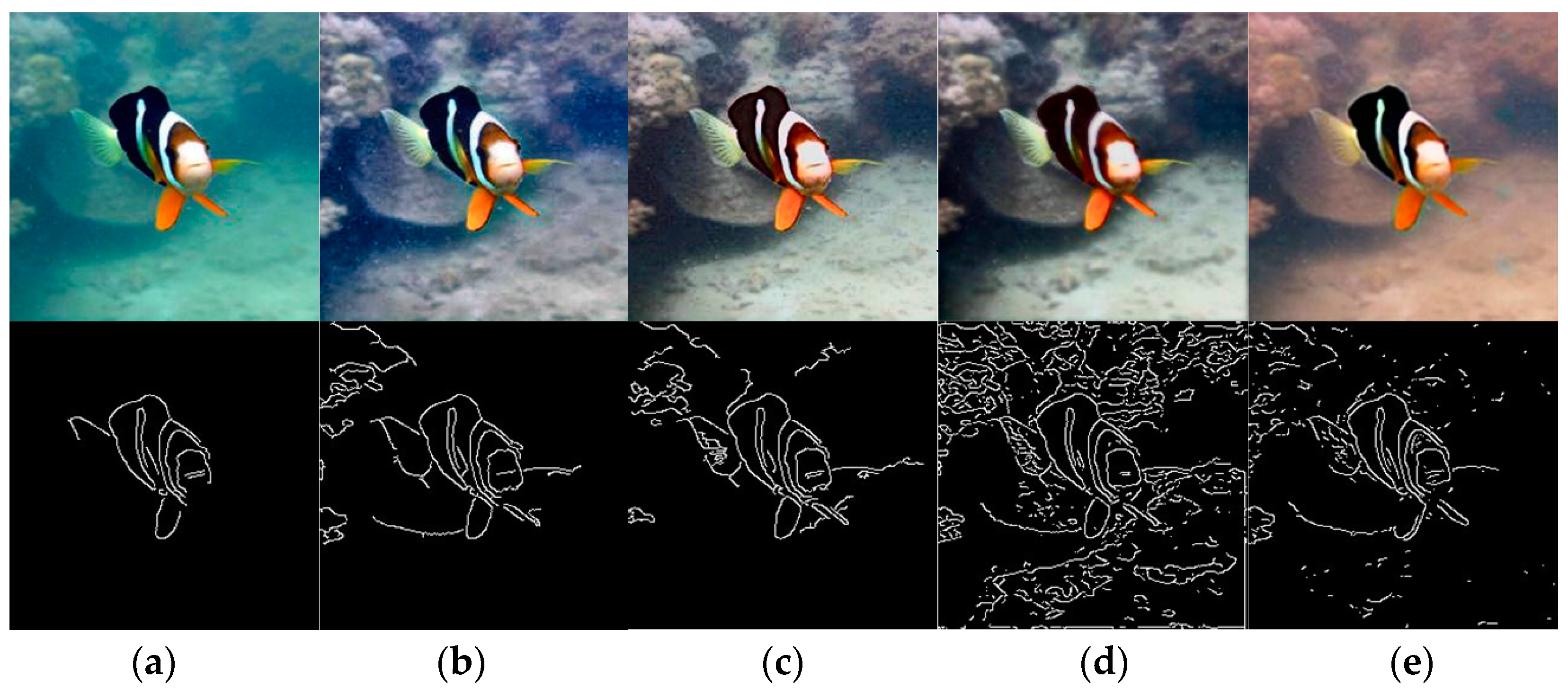
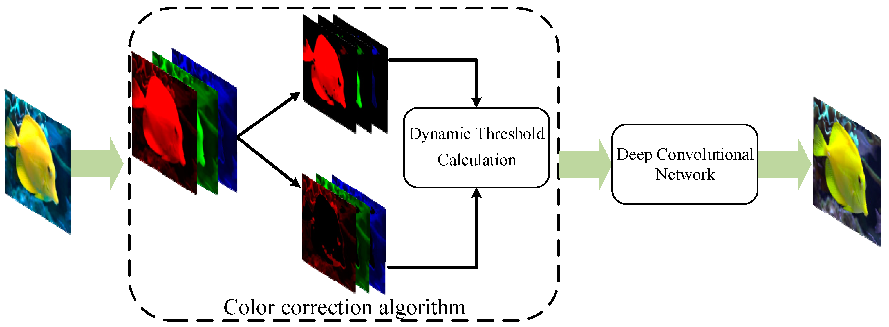
In terms of traditional methods, a novel dynamic color correction algorithm is developed based on the widely used gray world algorithm to restore the color of underwater image, which incorporates depth of field estimation. Initially, the depth of field for both the target and the background is estimated by analyzing the color attenuation difference. Subsequently, a dynamic threshold is devised for precise local segmentation. Finally, the degraded image is pretreated with the improved color correction method, thereby reducing the attenuation of underwater image color.

(3)

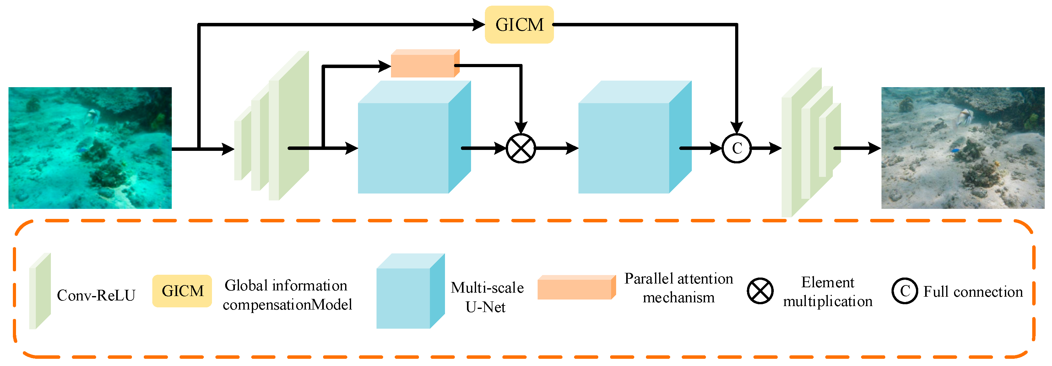
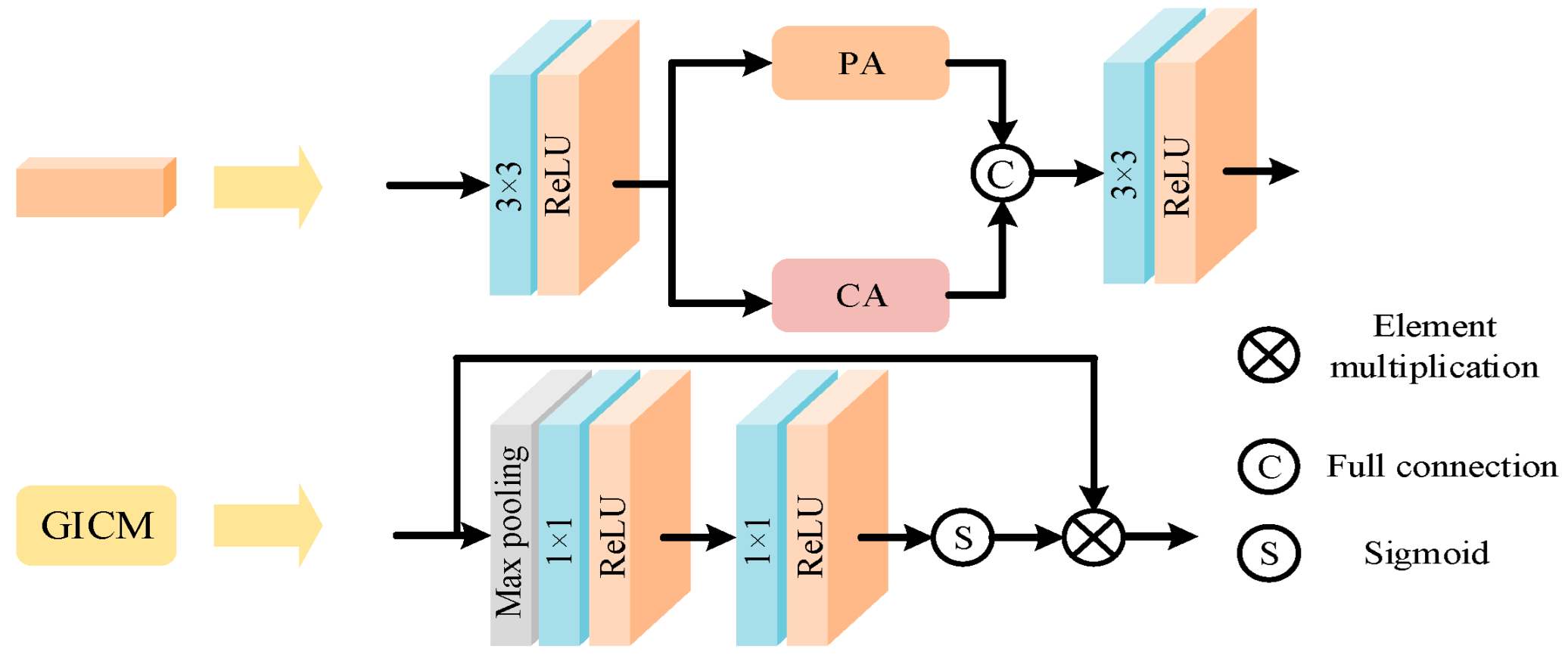
In deep learning networks, we have designed a multi-scale U-Net to increase the depth of convolutional networks and improve their ability to extract deep information from images. Additionally, we have introduced a parallel attention mechanism for adaptive learning of key spatial features, optimizing network parameters, and enhancing learning capabilities. This integration significantly boosts the model’s precision in distinguishing deep semantics, including intricate details and textures.

(4)

We propose a global information compensation algorithm to improve the network’s capacity to capture spatial information and enhance image integrity. By combining multiple loss functions, we also improve the network’s robustness and generalization ability for real underwater degraded images.

2. Related Work

In this section, we delve into the related algorithms for underwater image restoration and enhancement, ranging from the classical gray world theory to the recently popular channel and pixel attention mechanisms. These algorithms furnish us with a substantial theoretical and methodological foundation to tackle the complexities of the underwater environment.

2.1. Color Correcion Algorithm Based on Gray World Principle

According to the gray world principle, for an image with diverse colors, the average values of its three RGB components should theoretically converge to be equal. However, in special environments, such as underwater, specific color channels often experience attenuation because of light absorption or scattering by the medium. To address this issue, researchers have effectively utilized the gray world principle to develop a variety of efficient color correction algorithms. Among them, the most widely applied methods are as follows:

According to the Lambert reflection model, when a color image is captured using cameras, monitors, and other optical imaging-based equipment, the resulting image can be accurately represented by the physical model given by the following formula:

$$I_k(x)={\displaystyle \underset{F}{\int }[S_k(\lambda )E(\lambda )R(x,\lambda )]d\lambda k=R,G,B}$$

(1)

where I_k represents the image value of the k channel of the image. The integral ∫_F is the range of the visible spectrum (380~780 nm). S_k represents the response coefficient of the optical imaging equipment in the k channel. E is the spectral power distribution of the light source, and R is the reflectivity of the object surface reflected to the imaging equipment. The subscripts x and λ represent wavelength and spatial coordinates, respectively.

In normal circumstances, when a perceived white object is targeted for photography, it appears warm in color and the resulting image will exhibit a red color cast. Nevertheless, it will still be perceived as white by the human eye. The primary reason for this phenomenon is that the human visual system maintains a “color constancy” towards the object, whereas imaging equipment only truly records the light information reflected or transmitted by the object after light from the light source strikes it. However, subsequent machine vision tasks must be based on the actual recorded images, making the color cast image a significant obstacle to work efficiency. To address the reduced efficiency caused by the color cast issue, color correction algorithms are necessary to enhance image quality [17].

The gray world algorithm is a widely used color correction algorithm that relies on the “gray world hypothesis”. This hypothesis posits that, in images with numerous color variations, the average values of the three color components (red, green, and blue) tend towards a single gray value. It is assumed that, generally, the average reflection of natural scenery on light has a constant average value, which is approximately “gray” [18]. The gray world algorithm applies this assumption to the image being processed. By doing so, it can eliminate the influence of ambient light from the image and reconstruct the original scene image. Subsequently, it adjusts the color according to Von Kries’s diagonal theory. The formula for this adjustment is

$$E={\displaystyle \underset{F}{\int }{S}_k(\lambda )E(\lambda )}.$$

(2)

Among them, $S_k(\lambda )$ and $E(\lambda )$ are generally unknown; that is, there is no further assumption that this will be a “pathological” problem. Therefore, the gray world algorithm assumes that the average reflectivity coefficient in the scene is a gray value k, expressed as

$$k={\displaystyle \int R(x,\lambda )dx}/{\displaystyle \int dx}$$

(3)

where k is a constant; it can be obtained in two ways:

(1)

Direct reference: take half of the maximum value of each channel, that is, k = 128;

(2)

$k=(\overline{R}+\overline{G}+\overline{B})/3$, $\overline{R}$, $\overline{G}$ and $\overline{B}$, respectively, represent the average values of the three channels of red, green, and blue.

In order to ensure the stable color distribution of the corrected image, the second method is usually used to calculate the k value, and then $E$ can be estimated by calculating the average value of three channels:

$$\begin{array}{l}{\displaystyle \int I_k(x)dx/}{\displaystyle \int dx}={\displaystyle \int {\displaystyle \underset{F}{\int }[S_k(\lambda )E(\lambda )R(x,\lambda )]d\lambda dx/}}{\displaystyle \int dx}\\ =({\displaystyle \int R(x,\lambda )dx}/{\displaystyle \int dx})\times {\displaystyle \underset{F}{\int }{S}_k(\lambda )}E(\lambda )\\ =k{\displaystyle \underset{k}{\int }{S}_k(\lambda )}E(\lambda )=kE\end{array}.$$

(4)

The specific calculation steps are as follows:

(a)

Calculating the average values ($\overline{R}$, $\overline{G}$, and $\overline{B}$) of the three channels of the image R, G, and B:

$$\{\begin{array}{l}\overline{R}=(1/N){\displaystyle \sum _{i=1}^N{R}_i}\\ \overline{G}=(1/N){\displaystyle \sum _{i=1}^N{G}_i}\\ \overline{B}=(1/N){\displaystyle \sum _{i=1}^N{B}_i}\end{array}$$

(5)

where N is the number of pixels in the image. Let the average gray value of the image be shown by

$$K=(\overline{R}+\overline{G}+\overline{B})/3.$$

(6)

(b)

The gain coefficients of R, G, and B channels are as follows:

$$K_r=K/\overline{R};K_g=K/\overline{G};K_b=K/\overline{B}.$$

(7)

$\overline{R}$, $\overline{G}$, and $\overline{B}$ are the corrected values of red, green, and blue components, respectively.

(c)

Adjust the pixel value of each R, G, and B channel of the image to an acceptable displayable range (0, 255).

2.2. Channel Attention Mechanism

The primary objective of channel attention is to establish channel weight information for feature images, ensuring that the network focuses its attention on the processing of significant channels. A notable example is the Squeeze-and-Exclusion network (SENet) introduced by Hu et al. [19] The structure, as illustrated in Figure 2, comprises three fundamental components: squeeze, excitation, and scale functions.

Squeeze: The feature size of a normal image is H × W × C, where H, W, and C represent the height, width, and number of channels of the feature image, respectively. When the network processes the image, the convolution layer takes into account its size and number of channels. To ensure the network focuses more on processing image channels, global average pooling is employed to modify the spatial dimensions of images from H × W × C to 1 × 1 × C. This adjustment allows subsequent convolutional processes to operate solely on the channels.

Excitation: After changing the image space size to 1 × 1 × C, this operation introduces a learnable multi-layer perceptron to generate corresponding weights for different channel features and reduces dimensions in the middle to reduce parameters.

Scale: This operation multiplies the weight output by the excitation part with the network input features, redistributes the weighted information to the original image features, and completes the re-calibration of the original features in the channel dimension.

2.3. Pixel Attention Mechanism

The pixel attention mechanism ensures the network’s concentration on pixel-level processing by establishing pixel weight information within the feature image. Among the various approaches, Qin et al. [20] provided a comprehensive explanation in their 2018 work on the FFA-net, which is schematically represented in Figure 3.

The method employed by this mechanism is akin to the channel attention approach. Specifically, the spatial dimensions of the feature image are modified from H × W × C to H × W × 1 through a convolution unit. This adjustment enables the subsequent network to focus on pixel-level processing within individual channels. Subsequently, the ReLU activation function is utilized to activate pixel features initially, which is followed by further extraction in conjunction with the convolution unit. Finally, the Sigmoid activation function is employed, and the pixel weight feature is combined with the original image feature weight through element multiplication. The processed pixel feature weight is then redistributed back to the original image. Compared with spatial attention, this module can provide more understanding and analysis at the pixel level, making it more suitable for pixel loss restoration tasks such as underwater image restoration.

3. Materials and Methods

This section mainly presents the method for underwater image color restoration and texture enhancement proposed in this paper. This method integrates an advanced theoretical framework and innovative algorithm design to more effectively address a series of inherent challenges in underwater imaging, as illustrated in Figure 4. Specifically, we first employ a color correction algorithm, which incorporates a dynamic threshold calculation strategy, to minimize color degradation and adaptively enhance color attenuation. Secondly, we design a dual-channel-based deep convolutional neural network to further enhance the degraded images. Finally, the enhanced image is generated. The following sections will elaborate on each component in detail.

3.1. Color Correction Method

Step 1: The attenuation formula of light propagation in water is

$${\overline{P}}_c=1/MH{\displaystyle \sum _{i=1}^H{\displaystyle \sum _{j=1}^M{P}_c(i,j)}},c\in \{R,G,B\}$$

(8)

where M and H are the length and width of the image; $P_c(i,j)$ is the pixel value of the image in row i and column j; and R, G, and B represent the red, green, and blue channels of the image. Then, according to the obtained numerical ranking, the channels corresponding to large, medium, and small average values are defined as $P_l$, $P_m$, and $P_t$, respectively, and are reserved for subsequent stretching channels.

Step 2: Calculate the segmentation threshold from the difference between $P_l$ and $P_m$(the number of pixels):

$$(P_l-\alpha )/(P_l-P_m)=P/MH$$

(9)

where P represents the number of pixels of the image within $[\alpha ,P_l]$ intervals. By sorting out the above formula, the threshold can be expressed as

$$\alpha =P_l-P(P_l-P_m)/MH$$

(10)

The specific calculation method is shown in Algorithm 1. Where R, G, and B, respectively, represent the three-channel pixels of the input image, R_mean, G_mean, and B_mean are the corresponding average values, and endpoint1 and endpoint2 represent the calculated dynamic threshold, that is, the algorithm first calculates the channel with large attenuation and then calculates the corresponding segmentation threshold by the method of Formula (10) and outputs it. RAM is used to calculate whether the image is blue or green, which is used for the statistics of future tasks.

Algorithm 1 Dynamic threshold calculation

Input: R_mean, G_mean, B_mean, R, G, B Output: endpoint1, endpoint2 1: if B_mean ≥G_mean:     big = B; mid = G; RAM = 1   else:     big = G; mid = B; RAM = 2 2: max = (big-mid).max() 3: min = (big-mid).min() 4: endpoint1 = (max-mid)/2 + min 5: endpoint2 = max return endpoint1, endpoint2

Step 3: According to the obtained threshold, the gain in the corresponding threshold interval is calculated as follows:

$$D_c^{1,2}={\displaystyle \sum _{i=1}^H{\displaystyle \sum _{j=1}^M{P}_c^{1,2}(i,j)}}/P_c,c\in \{P_m,P_t\}$$

(11)

where $D^1$ and $D^2$, respectively, correspond to the gains of ($\alpha -P_t$) and ($P_l-\alpha$) intervals, and $p_c^{1,2}$ is the average pixel value of the corresponding interval.

Step4: The final correction formula is as follows:

$$\begin{array}{l}{P}_c^{CR}=P_c(i,j)+D_c\times P_l(i,j),\\ \hspace{1em}\hspace{1em}c\in \{P_m,P_t\},D=Min(D^1,D^2)\end{array}$$

(12)

The correction effect is shown in Figure 5. It can be seen that this method can not only effectively stretch the range of color channels, but also segment the target and background more stably, to better realize color correction according to the segmentation results.

3.2. Deep Learning Network

In this paper, we present the design of a deep convolutional network structure consisting of two primary components. The primary branch is a deep convolutional network, whose essence lies in enhancing the capability of feature learning from both degraded and clear images, as well as facilitating nonlinear transformations of deep semantic information by increasing the depth of the network. Additionally, the second branch is the global information compensation algorithm that directly extracts global and shallow features from the input features, thus effectively mitigating the issue of information loss in the deep convolutional network. The detailed structure is illustrated in Figure 6.

In the main branch, the core components of the deep convolution network include a multi-scale U-Net and parallel attention module. Figure 7 shows the structure of the deep convolution block. Firstly, the module extracts the spatial information of the input image step by step through a series of convolution units, including 7 × 7, 5 × 5, 3 × 3, and 1 × 1. Then, these feature images are restored correspondingly at the restoration end, which ensures the integrity of spatial semantic information. To further optimize the network parameters and performance, we used a 1 × 1 convolution unit to reduce the dimension. In addition, we introduce the Leaky-ReLU activation function to prevent the loss of details caused by the necrosis of output neurons in the negative half and, at the same time, improve the activity of transmission. This is helpful for the effective transmission of the weights of deep convolutional neural networks.

In deep convolutional networks, with the increase in network depth, it becomes difficult to update the weight information, which may lead to over-fitting or gradient explosion problems. To solve these problems, we introduce parallel attention blocks into the network structure, as shown in Figure 8. The structure is composed of channel attention (CA) and pixel attention (PA) modules in parallel, and a convolution unit is added to it to further extract the weights of pixels and channels. The main function of CA is to calculate and distribute the weights of image information in three channels, while PA is responsible for distributing the weights between pixels.

As shown in Figure 8, our Global Information Compensation Model (GICM) aims to enhance the capabilities of the backbone network to maintain the integrity of the image. Initially, the module employs a max-pooling operation to aggregate prominent features from the neighboring regions, thus retaining the texture features of the image. To ensure the uniformity of the output image, we configured the feature map to have a single output channel. Subsequently, we applied the Sigmoid activation function for output generation. Finally, we fused the input and output images via element-wise multiplication. By multiplying elements, we can merge two feature graphs with different dimensions to ensure their consistency in spatial dimension. In addition, this operation can also make the output image smoother, thus maintaining visual integrity.

3.3. Loss Fusion

Given the serious problems of edge and texture in degraded underwater images, the Laplacian operator is used as the main loss function in this chapter, and the template is

$$\left(\begin{array}{ccc}1& 1& 1\\ 1& -8& 1\\ 1& 1& 1\end{array}\right)$$

(13)

for the operation on the output of this chapter’s algorithm, which obtains $L(J^{\prime }(i))$. Then, we performed the Laplace operation on the corresponding clear image to obtain $L(J(i))$. Finally, the mean square error was used to calculate the loss, and the formula is

$$V_{\mathrm{Lap}}=\frac{1}{N}{\displaystyle \sum _{i=1}^N(L{(J^{\prime }(i)-L(J(i)))}^2}$$

(14)

where N represents the total pixel amount of the image and i represents the pixel position. In addition to detail, the problem of content loss is usually regarded as consistent with pixels, so perceptual loss is added to evaluate the capacity for feature reconstruction of underwater images, and the formula is

$$V_{\mathrm{perceptual}}=\frac{1}{C_j{H}_j{W}_j}{\Vert {\phi }_j(J_{gt})-{\phi }_j(J)\Vert }_2^2.$$

(15)

The total loss function of the proposed algorithm can be obtained as follows:

$$L=\alpha (V_{\mathrm{Lap}}+\lambda V_{\mathrm{perceptual}}).$$

(16)

Here, α is used to further improve the regularization ability of the loss function and is set to 1.5. After many experiments, the coefficient of weight λ was set to 0.1.

3.4. Training Details

Experimental platform: The GPU was NVIDIA RTX A4000 (16 GB). The CPU was Intel Core i9 13900h (2.6–5.4 GHz)—32 GB of running memory and Ubuntu 20.04 system.

The network was trained using the RGB channel. To enhance data diversity, we randomly rotated the input images by 90, 180, and 270 degrees and horizontally flipped them during training. We set the batch size to 2 and the crop size to 256, meaning two 256 × 256 images were fed into the network simultaneously. To ensure rapid and stable convergence, we used Adam as the optimizer and employed a cosine annealing strategy to adjust the learning rate. Initially, the learning rate was set to 1 × 10⁻³, which was then periodically reduced following the cosine curve during subsequent training. According to reference [21], this method not only assists the model in escaping local optimum solutions but also enhances the convergence rate of the network. The specific formula for the cosine annealing strategy is as follows:

$$Ir=0.5\times Ir\_\max \times (1+\cos (\frac{epoch}{epoch\_\max \times \pi }\left)\right)$$

(17)

where Ir indicates the current learning rate, Ir_max indicates the maximum learning rate, epoch indicates the number of rounds currently trained, and epoch_max indicates the total number of rounds to be trained. To select the optimal solution for the network, this paper also selectively stores the training model according to the test results of the verification set in SSIM (Structural Similarity Index) [22] and PSNR (Peak Signal-to-Noise Ratio) [23], and the pseudocode is shown in Algorithm 2. The inputs J’(x) and J(x) represent the output of our method and the real clear image, respectively, and the output model represents the stored pre-training model. This method mainly chooses whether to store the pre-training model by calculating the output SSIM and PSNR indicators.

Algorithm 2 Threshold calculation strategy

Input: J’(x), J(x) Output: model 1: PSNR_max = 0, SSIM_max = 0 2: for i in epoch_max: 3:  PSNR = VPSNR(J’(x), J(x)) 4:  SSIM = VSSIM(J’(x), J(x)) 5:  if SSIM>SSIM_max and PSNR > PSNR_max 6:   SSIM_max > SSIM, PSNR_max = PSNR 7:   model = model(i) 8:  end if 9: end for 10: return model

4. Experiment and Analysis

To verify the effectiveness of the proposed algorithm, we made subjective and objective evaluations on UFO, EUVP, and UIEB (Under water Image Enhancement Benchmark) [24] data sets, respectively, to prove the learning ability of the proposed network and its robustness in real underwater degradation environments with features such as greenness, blueness, low illumination, and fog. UFO, a synthetic data set specifically designed to provide corresponding clear images as a standard reference, contrasts with EUVP and UIEB, which are data sets containing real underwater images. In the allocation of the training set and test set, we adopted the strategy as shown in

Table 1. Allocation strategy of the training and test set.

Data Set	EUVP	UIEB
Sun	3000	700
Training set	2500	660
Test set	500	40

. In this way, we could evaluate the performance of the algorithm more comprehensively and ensure its good robustness in various underwater degradation environments.

The comparison algorithms are as follows: traditional methods include ICCB (2019), BRUE (2021), ACDC [25] (2022), and ULV [26] (2023); the deep learning algorithms include UDNet [27] (2018), FunIE [28] (2020), BLTM [29] (2020), DLIFM (2021), UWCNN (2021), and Semi-Net [30] (2023).

4.1. Subjective Evaluation

Figure 9 shows the test results of the algorithm in the degraded color card from the comparison results.

It can be seen that various algorithms show different advantages and disadvantages when processing color card images. The color card processed by the ICCB algorithm has different degrees of color deviation, which leads to the influence of color accuracy. The result of the BRUE algorithm is dark, and it shows poor robustness when dealing with dark colors, so it is difficult to maintain the authenticity of colors. The ULV algorithm and ACDC algorithm distort the color information of the image, produce a lot of noise, and seriously reduce the visual quality of the image. The results of the UWCNN algorithm and UDNet algorithm are too dark and fuzzy, which affects color reproduction. The FUnIE and BLTM algorithms perform well in vision tasks, but their ability to distinguish between yellow and green color cards is limited, leading to unclear color discrimination. The DLIFM algorithm further degrades the quality of the resulting image, while the Semi-Net algorithm corrects the color of the color card image, but the resulting image is blurry. In contrast, our proposed algorithm generates images with a blue tint that does not accurately represent the true colors of the color card. The algorithm presented in this study excels in color card image processing. It ensures that the color card image is bright and that each series’ colors are clearly distinguishable. The processed image’s colors closely resemble those of the actual color card, preserving its authenticity and color accuracy. When compared to other algorithms, our algorithm demonstrates superior performance in processing color card images and provides more precise and distinct color information, thereby enhancing the visual impact of images

The test results of related algorithms on UFO data sets [30] are shown in Figure 10. The UFO data set comprises pairs of underwater images. Conducting tests on this data set provides insights into the algorithm’s learning ability, as well as its processing effectiveness and stability in a typical underwater degradation environment. Through comparative analysis, we can observe the advantages and disadvantages of various algorithms in processing underwater images. The resulting image of the ICCB algorithm shows obvious color deviation, which leads to serious color distortion. Although the color of the BRUE algorithm is cold, it does not control the introduction of noise. The ACDC algorithm does not perform well in restoring the normal color of the image, and the overall tone is gray. The ULV algorithm presents different degrees of color deviation problems, such as green and blue; the FUnIE algorithm can solve the problem of dark images, but the resulting image appears with a yellow color cast; and the UWCNN algorithm also has serious color cast problem. At the same time, the UDNet algorithm also shows the problem of green and yellow color deviation. However, although the BLTM algorithm has solved the problem of image color cast stably, and the resulting image brightness is appropriate, the green color cast still appears in some areas. In addition, the resulting image from Semi-Net is dark as a whole. Relatively speaking, the algorithm proposed in this paper not only significantly improves the color cast problem of degraded images but also makes the images more vivid in color and clearer in detail. In terms of visual effect, compared with other algorithms, the color of the image obtained by the proposed method is closer to a real and clear image, and it exhibits higher stability in environments with synthetic color shifts and blurred atomization.

In Figure 11 and Figure 12, we present the experimental results of underwater images degraded with a predominance of blue and green hues, selected from the real underwater degraded image data set UIEBD. It can be observed that the ICCB algorithm and ULV algorithm have some limitations in dealing with the degradation of blue and green, and it is difficult to effectively correct the color cast. Although the BRUE algorithm can alleviate the problem of a color cast to some extent, the overall image is dark, which affects the improvement of the visual effect. The resulting image of the ACDC algorithm tends to be gray, so fails to accurately restore the image color. There is obvious distortion in the processing of the UDNet algorithm, which leads to a decline in image quality.

Compared with the above algorithms, FUnIE, UWCNN, Semi-Net, and BLTM algorithms show superior performance in dealing with color cast problems. However, they also introduce extra color casting in some images, which affects their overall performance to some extent. In contrast, our proposed algorithm shows better performance when dealing with degraded underwater images with bluish and greenish colors. This algorithm can not only effectively correct the color cast but also further improve the visual quality of the image, making the processed image clearer and more colorful. This fully proves the superiority and practicality of the algorithm in dealing with underwater degraded images.

Figure 13 and Figure 14 show the experimental results of each correlation algorithm when processing the images under low illumination and foggy water in the real data set UIEBD. It can be observed that the ICCB algorithm performs well in dealing with slight fog phenomena and alleviating low illumination, but its effect is greatly reduced in the face of dense fog environments or poor lighting conditions, which are prone to overexposure. BRUE and ACDC algorithms show some effect in dealing with the fog problem of underwater images, but unfortunately they are all accompanied by different degrees of color deviation, which affects the color accuracy of the images. ULV, FUnIE, Semi-Net, and BLTM algorithms all had poor performance in processing fog-degraded images; at the same time, they also had color cast problems in processing degraded underwater images with low illumination, which undoubtedly limits their practical application effect. The UWCNN algorithm has made some achievements in solving the degradation problem of atomized images, but the contrast of the resulting images is too high, which leads to the loss of some image information, which also harms its overall effect.

Compared to other methods, the algorithm introduced in this study demonstrates superior performance in handling degraded images. It not only enhances the brightness and saturation of the image, making it easier to distinguish background and target information but also addresses the issue of image fogging more effectively. This leads to a significant improvement in the utilization of image information processed by this algorithm, providing a more reliable foundation for subsequent image processing and analysis. Based on the above comparison results, we can see that our algorithm not only performs well in the synthetic data set but also has a more stable and effective effect compared with the other algorithm when dealing with complex underwater conditions such as blue, green, fog, and low illumination. This demonstrates our algorithm’s superior stability across various underwater environments. The remarkable success of the HA-Net method in processing underwater images is attributed to its dynamic color correction algorithm. This algorithm effectively reduces color distortion in underwater images, enhancing color fidelity and visual quality. Additionally, the combination of multi-scale U-Net and the parallel attention mechanism significantly improves the network’s accuracy in recognizing deep semantics, especially when handling fine textures. Furthermore, the global information compensation algorithm, incorporating various loss functions, enhances image integrity and boosts the network’s ability to capture spatial information, as well as its robustness in handling real underwater images.

4.2. Objective Evaluation

To further validate the performance of the proposed algorithm, we conducted objective evaluations on the results obtained from the algorithm and comparison algorithms using UFO, EUVP, and UIEB data sets. Notably, UFO is a synthetic data set that provides corresponding clear images as a standard reference. Given this feature, we used SSIM and PSNR as reference indicators to evaluate the performance of the algorithm in image restoration. EUVP and UIEB are real underwater image data sets, which can better reflect the robustness of the algorithm in a real environment. For these two data sets, we used NIQE (Natural Image Quality Evaluation) [31], UIQM (Underwater Image Quality Measures [32]), and CEIQ (Color Enhanced Image Quality [33]) for evaluation. These non-reference indexes can objectively evaluate the image quality after algorithm processing without relying on the original clear image. To further increase the persuasiveness of the experiment, we also used the above-mentioned non-reference indicators for objective testing on UFO data sets. The purpose of doing this was to verify the consistency and effectiveness of non-reference indicators on different types of data sets, and to evaluate the performance of the algorithm in this paper more comprehensively. Through the application of this series of experimental design and evaluation indicators, we expect to measure the performance of the proposed algorithm in dealing with underwater degraded images more accurately.

The evaluation results for the UFO data set are presented in

Table 2. Evaluation index results of the UFO data set. (“↑” indicates that the bigger the index, the better; “↓” indicates that the smaller the index, the better; bold represents the optimal value.)

	SSIM↑	PSNR↑	NIQE↓	UIQM↑	CEIQ↑
Degraded	0.75	20.10	4.58	3.67	2.85
ICCB	0.69	18.31	4.99	4.16	3.66
BRUE	0.51	13.54	5.87	5.13	3.57
ACDC	0.60	18.71	6.51	5.14	3.47
ULV	0.71	17.95	5.98	5.84	3.14
UDNet	0.39	12.88	5.25	4.62	3.24
FUnIE	0.71	21.51	4.87	3.54	3.36
BLTM	0.79	22.94	3.77	6.11	3.44
UWCNN	0.73	20.58	4.95	4.97	3.54
Semi-Net	0.81	23.37	3.84	5.17	3.12
HA-Net	0.85	23.89	3.50	5.24	3.89

, where the bolded items represent optimal performance. Clearly, based on the evaluation results from the UFO data set, our proposed algorithm has achieved the highest scores in both SSIM and PSNR. This suggests that the output images closely resemble clear, realistic data, specifically in terms of their structural similarity and signal-to-noise ratio. Such results strongly demonstrate the excellence of our proposed algorithm in image processing. Compared to other methods, our algorithm excels in efficiently restoring high-quality underwater imagery. Furthermore, the assessment results for the non-reference metrics CEIQ, NIQE, and UIQM also indicate that our method has reached optimal levels in these areas. This underscores that our algorithm not only performs well in terms of natural authenticity, clarity, and color fidelity but also surpasses the benchmark algorithm in overall performance across all metrics. These objective assessments strongly endorse the efficacy and superiority of our proposed algorithm. Additionally, the evaluation results for the EUVP and UIEBD data sets are shown in

Table 3. valuation index results of the EUVP and UIEBD data set. (“↑” indicates that the bigger the index, the better; “↓” indicates that the smaller the index, the better; bold represents the optimal value.)

	EUVP			UIEBD
	NIQE↓	UIQM↑	CEIQ↑	NIQE↓	UIQM↑	CEIQ↑
Degraded	4.68	3.67	3.56	5.53	1.04	3.95
ICCB	6.63	4.25	3.66	6.85	1.26	3.69
BRUE	6.44	5.13	3.47	8.07	1.58	3.47
ACDC	4.02	5.10	3.14	6.47	2.01	3.44
ULV	7.84	2.14	3.74	9.89	2.32	3.14
UDNet	4.31	4.65	3.65	6.84	1.85	3.05
FUnIE	3.77	5.14	3.28	5.64	3.16	3.85
BLTM	4.26	4.81	3.77	6.12	3.02	3.62
UWCNN	3.81	5.22	3.55	5.71	4.22	3.42
Semi-Net	3.34	5.37	3.84	5.52	4.07	3.77
HA-Net	3.11	6.01	3.88	5.00	4.16	3.83

.

Judging from the evaluation results of EUVP data sets, all the indexes of our algorithm are better than those of the contrast algorithm, which demonstrates comprehensively that our method is more stable in real data sets. Although the UIEBD data set has not been clarified, which leads to our method being inferior to the original image in the CEIQ index, compared with other algorithms, our method still shows superiority. It is worth noting that the UIQM value of this method is 4.16, which is second only to the UWCNN algorithm but superior to other algorithms in other indexes. This result further proves the stability of this method in maintaining image quality. On the whole, the robustness and generalization ability of this algorithm in a real environment has been fully verified. Whether synthetic or real data sets are used, this method demonstrates excellent performance and offers an effective solution to the problem of underwater image degradation.

4.3. Ablation Study

To further verify the effectiveness of each module proposed in our method, we carefully designed ablation experiments on UFO data sets. By gradually introducing or removing specific modules, we can more accurately evaluate the contribution of each module to the overall performance. At the same time, to show the experimental results intuitively, we combined SSIM, PSNR, NIQE, and UIQM to comprehensively evaluate the image quality. The specific experimental arrangements are as follows. We introduced the ablation situation of each module one by one, and reveal the key role of each module in improving image quality by comparing the experimental data:

(1)

w/o CCM: the degraded image is directly input to the network for training and testing without using the color correction method for preprocessing.

(2)

w/o MSU-Net: instead of using multi-scale U-Net to extract cyberspace information, it is replaced by a six-layer general convolution structure.

(3)

w/o GICM: the Global Information Compensation Model is not applicable.

(4)

w/o PAM: do not use the parallel attention mechanism.

(5)

HA-Net: use the full structure of this paper network.

The experimental results are shown in

Table 4. Test results of the ablation experiment. (“↑” indicates that the bigger the index, the better; “↓” indicates that the smaller the index, the better; bold represents the optimal value.)

Method	SSIM↑	PSNR↑	NIQE↓	UIQM↑
w/o CCM	0.84	19.88	5.12	3.41
w/o MSU-Net	0.75	20.56	3.25	5.10
w/o GICM	0.83	21.85	4.55	4.84
w/o PAM	0.87	19.38	4.87	5.07
HA-Net	0.95	24.89	3.47	5.31

. It can be seen that due to the lack of data set preprocessing, it is difficult to suppress the nonlinear degradation problem of degraded images, which leads to the difficulty of network learning, so the evaluation index of w/o CCM is the lowest. However, it is difficult for the network lacking a multi-scale U-Net to extract deep semantic information, the network lacking a global information compensation algorithm to ensure the stability and integrity of the image, and the network lacking a parallel attention mechanism to calculate the uneven degradation weight, which makes it difficult to restore the image stably. In contrast, the complete HA-Net fully integrates the advantages of each module and achieves the optimal value.

4.4. Application Experiment

In this section, we elaborate on the performance of our method in real-world application scenarios, including object detection, gradient map experiments, and saliency detection. We verify its effectiveness through experiments. Referring to Figure 15, we present the experimental outcomes of the YOLOv7 [34] algorithm on both the original degraded images and the enhanced clear images that were processed by various algorithms. Notably, FUnIE exhibits the lowest confidence score among all the compared algorithms across all three images, even lower than the score of the original degraded image. While the ICCB algorithm enhances the confidence scores solely on the first image, it does not significantly elevate the image quality. Although the ULV, BLTM, and Semi-Net algorithms yield better confidence scores than the original degraded images in some instances, they produce more misdetected targets compared to our method and are visually unsatisfying. In the second image, despite our algorithm slightly trailing the BLTM algorithm in color reproduction, it attains an impressive confidence level of 0.74, surpassing all other compared algorithms. However, in the third image, our method’s confidence level dips to 0.60, performing considerably below the top-performing Semi-Net algorithm and even falling behind the original degraded image. To enhance the stability of the algorithm, we intend to take two approaches for improvement. First, we aim to optimize and expand the training data set, thereby improving the algorithm’s adaptability to various degradation scenarios. Second, we intend to adjust the network structure and parameter settings to bolster the algorithm’s robustness when tackling complex degradation situations. Through these measures, we aspire to further elevate the performance and stability of the algorithm in our future work. In summary, this algorithm not only improves the visual quality of degraded images but also provides a more accurate and reliable database for subsequent target detection tasks.

We conducted gradient map edge detection experiments on both the original image and the image processed by the algorithm. The experimental results show a direct correlation between the clarity of texture features in the image and the number of edges detected. Specific experimental results are shown in Figure 16. Through comparative analysis, it can be clearly observed that, in terms of gradient map edge detection, the image enhanced by the algorithm is significantly better than the original image, successfully detecting more edge details. This discovery fully demonstrates the effectiveness of the algorithm described in this chapter in enhancing image texture details, thereby significantly improving the clarity of the image. In summary, this algorithm not only improves image quality but also demonstrates broad application potential and value in other visual inspection fields in the future.

The experimental results show that the image quality has been significantly improved by using this algorithm, which means that the diver’s legs, which were originally ignored, are also highly noticeable in the processed image. This further proves the effectiveness of the algorithm in enhancing image clarity. Figure 17 shows the results of this remarkable experiment. After a thorough analysis of the experiments mentioned above, it is clear that our algorithm has demonstrated superior performance in both subjective and objective comparisons, as well as in various application scenarios. However, when faced with certain degraded images featuring large areas of identical colors, the algorithm’s performance still needs improvement. Therefore, our next focus will be on adjusting the training data set and optimizing the algorithm to enhance the stability and applicability of our approach.

5. Conclusions

Aiming to tackle the challenges faced by existing traditional and deep learning algorithms in stably restoring degraded images of complex underwater environments, we propose a hybrid algorithm model for underwater image color restoration and texture enhancement. In this method, we introduce a new dynamic color correction algorithm based on depth of field estimation that can accurately correct the color according to the adaptive threshold of the target and background, thus effectively preprocessing the image. In addition, we constructed a multi-scale U-Net structure and integrated the parallel attention mechanism. This combination can not only mine the deep semantic information of the image thoroughly but also accurately extract weight information according to the unique nonlinear and uneven degradation characteristics of the underwater image, thus significantly improving the quality. To ensure the integrity of the output image, we also carefully designed the global information compensation algorithm. By precisely adjusting the loss function, we can ensure that the image output by the network is rich in detail and intact as a whole. The experimental results show that our method is obviously superior to other novel and classical methods in subjective visual evaluation and objective index comparison. The SSIM and PSNR values in the synthetic data set named UFO reached 0.85 and 23.89, respectively. Additionally, for the real data set UIEBD, our approach yielded NIQE and UIQM scores of 5.00 and 4.16, respectively. Moreover, within the EUVP data set, our method secured NIQE and UIQM scores of 3.11 and 6.01, respectively, demonstrating higher evaluation results when compared to the benchmark algorithm in terms of overall image quality assessment. The ablation experiment further validated the effectiveness and contribution of our modules. Additionally, we conducted practical application tests, which showed that the proposed algorithm exhibits significant advantages in real-world marine environments. In the future, our focus will be on introducing more prior knowledge to further enhance the generalization capabilities and robustness of the algorithm in complex and dynamic environments, ensuring its efficiency and stability under various conditions.

References

1. Qian, J.; Li, H.; Zhang, B.; Lin, S.; Xing, X. DRGAN: Dense Residual Generative Adversarial Network for Image Enhancement in an Underwater Autonomous Driving Device. Sensors 2023, 23, 8297. [Google Scholar] [CrossRef] [PubMed]
2. Lai, Y. A comparison of traditional machine learning and deep learning in image recognition. J. Phys. Conf. Ser. 2019, 1314, 012148. [Google Scholar] [CrossRef]
3. Iqbal, K.; Salam, R.A.; Osman, A.; Talib, A.Z. Underwater Image Enhancement Using an Integrated Colour Model. IAENG Int. J. Comput. Sci. 2007, 34, 239–244. [Google Scholar]
4. Ancuti, C.O.; Ancuti, C.; De Vleeschouwer, C.; Bekaert, P. Color balance and fusion for underwater image enhancement. IEEE Trans. Image Process. 2017, 27, 379–393. [Google Scholar] [CrossRef] [PubMed]
5. Nomura, K.; Sugimura, D.; Hamamoto, T. Underwater image color correction using exposure-bracketing imaging. IEEE Signal Process. 2018, 25, 893–897. [Google Scholar] [CrossRef]
6. Zhang, W.; Pan, X.; Xie, X.; Li, L.; Wang, Z.; Han, C. Color correction and adaptive contrast enhancement for underwater image enhancement. Comput. Electr. Eng. 2021, 91, 106981. [Google Scholar] [CrossRef]
7. Zhao, C.; Cai, W.; Dong, C.; Hu, C. Wavelet-based fourier information interaction with frequency diffusion adjustment for underwater image restoration. In Proceedings of the IEEE/CVF Conference on Computer Vision and Pattern Recognition, Seattle, WA, USA, 17–21 June 2024; pp. 8281–8291. [Google Scholar]
8. Lu, H.; Li, Y.; Uemura, T.; Kim, H.; Serikawa, S. Low illumination underwater light field images reconstruction using deep convolutional neural networks. Future Gener. Comp. Sy. 2018, 82, 142–148. [Google Scholar] [CrossRef]
9. Gangisetty, S.; Rai, R.R. FloodNet: Underwater image restoration based on residual dense learning. Signal Process. Image Commun. 2022, 104, 116647. [Google Scholar] [CrossRef]
10. Lu, J.; Yuan, F.; Yang, W.; Cheng, E. An imaging information estimation network for underwater image color restoration. IEEE J. Ocean. Eng. 2021, 46, 1228–1239. [Google Scholar] [CrossRef]
11. Yang, M.; Hu, K.; Du, Y.; Wei, Z.; Sheng, Z.; Hu, J. Underwater image enhancement based on conditional generative adversarial network. Signal Process. Image Commun. 2020, 81, 115723. [Google Scholar] [CrossRef]
12. Wang, H.; Sun, S.; Chang, L.; Li, H.; Zhang, W.; Frery, A.C.; Ren, P. INSPIRATION: A reinforcement learning-based human visual perception-driven image enhancement paradigm for underwater scenes. Eng. Appl. Artif. Intell. 2024, 133, 108411. [Google Scholar] [CrossRef]
13. Wang, G.; Tian, J.; Li, P. Image color correction based on double transmission underwater imaging model. Acta Opt. Sin. 2019, 39, 0901002. [Google Scholar] [CrossRef]
14. Zhuang, P.; Li, C.; Wu, J. Bayesian retinex underwater image enhancement. Eng. Appl. Artif. Intell. 2021, 101, 104171. [Google Scholar] [CrossRef]
15. Liu, R.; Fan, X.; Zhu, M.; Hou, M.; Luo, Z. Real-world underwater enhancement: Challenges, benchmarks, and solutions under natural light. IEEE Trans. Circuits. Syst. Video Technol. 2020, 30, 4861–4875. [Google Scholar] [CrossRef]
16. Liu, X.; Gao, Z.; Chen, B.M. MLFcGAN: Multilevel feature fusion-based conditional GAN for underwater image color correction. IEEE Geosci. Remote Sens. Lett. 2019, 17, 1488–1492. [Google Scholar] [CrossRef]
17. Singh, M.; Sharma, D.S. Enhanced color correction using histogram stretching based on modified gray world and white patch algorithms. Int. J. Comput. Sci. Inf. Technol. 2014, 5, 4762–4770. [Google Scholar]
18. Pan, B.; Jiang, Z.; Zhang, H.; Luo, X.; Wu, J. Improved gray world color correction method based on weighted gain coefficients. Optoelectron. Imaging Multimed. Technol. III 2014, 9273, 625–631. [Google Scholar]
19. Hu, J.; Shen, L.; Sun, G. Squeeze-and-excitation networks. In Proceedings of the IEEE Conference on Computer Vision and Pattern Recognition, Salt Lake City, UT, USA, 18–22 June 2018; pp. 7132–7141. [Google Scholar]
20. Qin, X.; Wang, Z.; Bai, Y.; Xie, X.; Jia, H. FFA-Net: Feature fusion attention network for single image dehazing. In Proceedings of the AAAI Conference on Artificial Intelligence, New York, NY, USA, 7–12 February 2020; pp. 11908–11915. [Google Scholar]
21. Johnson, O.V.; Chen, X.; Khaw, K.W.; Lee, M.H. ps-CALR: Periodic-Shift Cosine Annealing Learning Rate for Deep Neural Networks. IEEE Access 2023, 11, 11908–11915. [Google Scholar] [CrossRef]
22. Mudeng, V.; Kim, M.; Choe, S.W. Prospects of structural similarity index for medical image analysis. Appl. Sci. 2022, 12, 3754. [Google Scholar] [CrossRef]
23. Yoo, J.C.; Ahn, C.W. Image matching using peak signal-to-noise ratio-based occlusion detection. IET Image Process. 2012, 6, 483–495. [Google Scholar] [CrossRef]
24. Drews, P.; Nascimento, E.; Moraes, F.; Botelho, S.; Campos, M. Transmission estimation in underwater single images. In Proceedings of the IEEE International Conference on Computer Vision Workshops, Sydney, Australia, 2–8 December 2013; pp. 825–830. [Google Scholar]
25. Zhang, W.; Wang, Y.; Li, C. Underwater image enhancement by attenuated color channel correction and detail preserved contrast enhancement. IEEE J. Ocean. Eng. 2022, 47, 718–735. [Google Scholar] [CrossRef]
26. Hao, Y.; Hou, G.; Tan, L.; Wang, Y.; Zhu, H.; Pan, Z. Texture enhanced underwater image restoration via Laplacian regularization. Appl. Math. Model. 2023, 119, 68–84. [Google Scholar] [CrossRef]
27. Pan, P.W.; Yuan, F.; Cheng, E. Underwater image de-scattering and enhancing using dehazenet and HWD. J. Mar. Sci. Technol. 2018, 26, 531–540. [Google Scholar]
28. Islam, M.J.; Xia, Y.; Sattar, J. Fast underwater image enhancement for improved visual perception. IEEE Robot. Autom. Lett. 2020, 5, 3227–3234. [Google Scholar] [CrossRef]
29. Song, W.; Wang, Y.; Huang, D.; Liotta, A.; Perra, C. Enhancement of underwater images with statistical model of background light and optimization of transmission map. IEEE Trans. Broadcast. 2020, 66, 153–169. [Google Scholar] [CrossRef]
30. Huang, S.; Wang, K.; Liu, H.; Chen, J.; Li, Y. Contrastive semi-supervised learning for underwater image restoration via reliable bank. In Proceedings of the IEEE/CVF Conference on Computer Vision and Pattern Recognition, Vancouver, BC, Canada, 18–22 June 2023; pp. 18145–18155. [Google Scholar]
31. Yang, M.; Sowmya, A. An underwater color image quality evaluation metric. IEEE Trans. Image Process. 2015, 24, 6062–6071. [Google Scholar] [CrossRef] [PubMed]
32. Panetta, K.; Gao, C.; Agaian, S. Human-visual-system-inspired underwater image quality measures. IEEE J. Ocean. Eng. 2015, 41, 541–551. [Google Scholar] [CrossRef]
33. Hu, K.; Zhang, Y.; Weng, C.; Wang, P.; Deng, Z.; Liu, Y. An underwater image enhancement algorithm based on generative adversarial network and natural image quality evaluation index. J. Mar. Sci. Eng. 2021, 9, 691. [Google Scholar] [CrossRef]
34. Wang, C.Y.; Bochkovskiy, A.; Liao, H.Y.M. YOLOv7: Trainable bag-of-freebies sets new state-of-the-art for real-time object detectors. In Proceedings of the IEEE/CVF Conference on Computer Vision and Pattern Recognition, Vancouver, BC, Canada, 18–22 June 2023; pp. 7464–7475. [Google Scholar]
Figure 1. Results of the correlation algorithm and its gradient diagram display: (a) degenerate image, (b) ICCB [13], (c) BRUE [14], (d) UWCNN [15], and (e) MLFcGAN [16].
Electronics 13 02623 g001
Figure 2. Structure diagram of channel attention.
Electronics 13 02623 g002
Figure 3. Structure diagram of pixel attention.
Electronics 13 02623 g003
Figure 4. Structure of our method.
Electronics 13 02623 g004
Figure 5. Related results of our color correction method are displayed.
Electronics 13 02623 g005
Figure 6. Structure of our deep learning network.
Electronics 13 02623 g006
Figure 7. Structure of multi-scale U-Net.
Electronics 13 02623 g007
Figure 8. Parallel attention mechanism and the structure of the Global Information Compensation Model.
Electronics 13 02623 g008
Figure 9. Comparison of experimental results of color cards.
Electronics 13 02623 g009
Figure 10. Test results of the UFO data set: (a) degenerate image, (b)ICCB, (c) BRUE, (d) ACDC, (e) ULV, (f) UDNet, (g) FUnIE, (h) BLTM, (i) UWCNN, (j) Semi-Net, (k) HA-Net, and (l) clear image.
Electronics 13 02623 g010
Figure 11. Test results obtained in a blue-colored test scene under actual conditions: (a) degraded image, (b) ICCB, (c) BRUE, (d) ACDC, (e) ULV, (f) UDNet, (g) FUnIE, (h) BLTM, (i) UWCNN, (j) Semi-Net, and (k) HA-Net.
Electronics 13 02623 g011
Figure 12. Test results obtained in a green-colored test scene under actual conditions: (a) degraded image, (b) ICCB, (c) BRUE, (d) ACDC, (e) ULV, (f) UDNet, (g) FUnIE, (h) BLTM, (i) UWCNN, (j) Semi-Net, and (k) HA-Net.
Electronics 13 02623 g012
Figure 13. Test results of low-light scene under actual conditions: (a) degraded image, (b) ICCB, (c) BRUE, (d) ACDC, (e) ULV, (f) UDNet, (g) FUnIE, (h) BLTM, (i) UWCNN, (j) Semi-Net, and (k) HA-Net.
Electronics 13 02623 g013
Figure 14. Test results of hazy scene under actual conditions: (a) degraded image, (b) ICCB, (c) BRUE, (d) ACDC, (e) ULV, (f) UDNet, (g) FUnIE, (h) BLTM, (i) UWCNN, (j) Semi-Net, and (k) HA-Net.
Electronics 13 02623 g014
Figure 15. YOLOv7 detection results of images before and after enhancement: (a) degraded image, (b) ICCB, (c) ULV, (d) FUnIE, (e) BLTM, (f) Semi-Net, and (g) HA-Net.
Electronics 13 02623 g015
Figure 16. Experimental results of gradient map before and after enhancement.
Electronics 13 02623 g016
Figure 17. Experimental results of significance detection.
Electronics 13 02623 g017