Impact of Multi-Energy System and Different Control Strategies on a Generic Low-Voltage Distribution Grid

Abstract

The rising electricity costs, cost of space heating, and domestic hot water end up driving consumers toward reducing expenses by generating their electricity through devices like photovoltaic systems and efficient combined heat and power plants. When coupled with thermal systems via an energy management system (EMS) in a Multi-Energy System (MES), this self-produced electricity can effectively lower electricity and heating bills. However, MESs with EMSs can serve various purposes beyond cost reduction via self-consumption, such as reacting to variable electricity prices, meeting special grid connection conditions, or minimizing CO₂ emissions. These diverse strategies create unique prosumer profiles, deviating significantly from standard load profiles. The potential threat to the power grid arises as grid operators lack visibility into which consumers employ which control strategies. This paper investigates the impact of controlled MESs on the power grid compared to average households and answers whether new control strategies affect the planning strategies of low voltage grids. It proposes a comprehensive four-step toolchain for the detailed simulation of thermal–electrical load profiles, MES control strategies, and grid dynamics. It includes a new method for the grid impact analysis of extreme and average bulk values. As a result, this study identifies three primary factors influencing distribution power grids by MESs. Firstly, the presence and scale of photovoltaic (PV) systems significantly affect extreme values in the grid. Secondly, MESs incorporating combined heat and power (CHP) and heat pump (HP) units impact the overall grid performance, mainly reflected in bulk values. Thirdly, the placement of an MES with heating systems, especially when concentrated in one feeder, plays a crucial role in grid dynamics. Despite the three distinct factors identified as impactful on the power grid, this study reveals that the various control strategies, despite leading to vastly different grid profiles, do not exhibit divergent impacts on buses, lines, or transformers. Remarkably, the impact of MESs remains consistently similar across the range of control strategies studied. Therefore, different control strategies do not pose an additional challenge to the grid integration of MESs.

1. Introduction

With the European Green Deal, the EU has set its climate aspirations high, aiming to achieve energy efficiency and emerge as the world’s first climate-neutral continent by 2050. Installing and integrating decentralized renewable energy systems, such as photovoltaic and wind parks, will play a pivotal role in realizing these ambitious targets. Over the past decade, numerous studies have delved into describing the impact and seamless integration of photovoltaic (PV) systems into power grids (refer to [1] for a comprehensive review). However, since the Russian aggression war against Ukraine and the subsequent energy crisis, there has been a sharp focus in politics and the economy on transforming the heating sector. The shift from inefficient gas and oil systems to efficient, electric-based heating solutions like heat pumps (HPs) and combined heat and power (CHP) plants is gaining momentum. Consequently, studies are now examining the integration of HP and CHP systems into the power grid alongside PV systems. Their integration depends on the usage and management strategies of the systems. A common method of controlling HP and CHP plants is through thermal-driven mechanisms, often in conjunction with buffer storage. These systems are activated when there is a thermal load demand or when the buffer storage temperature falls below a certain threshold. The fusion of PV and HP systems to mitigate electricity costs hinges on self-consumption. Ref. [2] introduced PV-driven HP control strategies aimed at maximizing PV self-consumption for HP operation. This concept was simulated using TRNSYS and successfully validated in a laboratory setting for a typical day in July. Moreover, HPs, as part of smart grids, offer additional control possibilities. Ref. [3] provided a review of HP applications in SmartGrids, evaluating three key use cases: (1) supporting stable and economical grid operation, (2) providing flexibility for the integration of volatile Distributed Energy Resources (DERs), and (3) operating under fluctuating electricity prices. This illustrates the vast array of control strategies of heating systems that can yield varying impacts on the power grid. The complexity further escalates with the introduction of multi-energy systems.

A multi-energy system (MES) integrates electrical and thermal energy components, functioning as a unified energy system. Within MES frameworks, diverse components such as PV systems, HP systems, combined heat and power plants (CHP), batteries, thermal storages, gas boilers, and electrical heaters operate synergistically. An MES offers improved performance compared to conventional separate energy systems [4]. However, the planning and operating of an MES entail complexity due to the variability in component combinations, which is contingent on factors like local weather conditions, energy demands, regulations, and control strategies. For instance, ref. [5] describes an MES optimization study aimed at minimizing total capital costs, operational costs, and shifting load compensation costs while ensuring system reliability and safety. Meanwhile, ref. [6] provides a comprehensive review outlining MES control and planning methods alongside existing modeling tools. The review encompasses top-down, bottom-up, and hybrid methodologies, along with various mathematical approaches such as linear programming, dynamic programming, mixed-integer programming, stochastic programming, and the utilization of artificial intelligence. These studies and the referees underscore the intricate nature of MES planning and operation, necessitating versatile approaches and robust modeling tools to effectively navigate these systems’ complexities.

Optimized controls, particularly Model Predictive Controls (MPC), exhibit a diverse array of applications for MESs, yielding heightened efficiency and reduced operational costs. In a comprehensive study detailed in [7], a prolonged investigation into MPC-controlled HP operation within a residential setting, coupled with PV power generation, spanned 135 days. The findings revealed a reduction in the electrical energy demand of the HP and an increase in the Coefficient of Performance (COP), resulting in a notable 9% reduction in energy costs. Similarly, studies examining PV-CHP systems [8,9,10] have corroborated these favorable outcomes. Kneiske et al. introduced a novel combined control algorithm for PV-CHP hybrid systems in [11], combining MPC with rule-based control. This innovative approach enables adjustments for deviations from perfect forecasts. The efficacy of the MPC algorithm was validated through bench testing [11]. All the different applications and control strategies of MESs mentioned prompt the following questions. What impact do these emerging flexible electric-thermal energy systems in households have on distribution grid infrastructure, particularly at the low voltage level? What are the primary factors and parameters that necessitate consideration in grid planning and operation?

Grid simulation studies on the impact of emerging technologies are typically conduct assessments using grid simulation tools. Frameworks for distribution grid planning have been outlined in studies such as [12,13]. These frameworks offer two planning methods: one based on extreme values, such as maximum installed PV capacities and loads, and the other employing a time-series-based approach. The latter method involves analyzing a designated time period, typically a year, and a defined resultion for time steps, utilizing PV and standard load profiles, which is particularly useful when smart-meter measurements are unavailable. Time-series simulations are crucial for assessing the influence of different MES types and control strategies. It is imperative not to use the standard load profiles but to derive accurate load profiles for various MES configurations to ensure realism and avoid the over or underestimation of their impact due to unrealistic consumption simultaneity. The comprehensive review in [14] highlights various methodologies for obtaining load profiles, each relying on different input information and calculation techniques and offering varying degrees of applicability. Approaches utilizing smart-meter measurements, aiming to capture specific load profile features [15] or providing anonymized datasets [16], hinge on the availability of representative datasets. Other data-driven approaches, such as those illustrated by Peters et al. [17], involve improving standard load profiles by comparing grid model load profiles with real measurement data. They found that generating a regional synthetic load profile from measured data significantly enhanced the accuracy compared to standard load profiles. Furthermore, the time resolution of load profiles is a critical factor. While standard load profiles typically exhibit resolutions ranging from 1 h to 15 min, studies like that of Bouvenot et al. [18] emphasize the importance of high-resolution time profiles compared to hourly data, particularly in accurately estimating micro-CHP electrical generation self-consumption rates. In modeling domestic hot water or space heating load profiles, detailed simulations using tools like TRNSYS, as demonstrated in [19], are common. However, research dedicated to thermal or heating load profiles remains relatively scarce. Therefore, it is essential to generate consistent load profiles for the household electrical demand, in conjunction with space heating and domestic hot water, to reflect the true household load profile. These profiles are distinct from the grid load profile, which aggregates all electrical consumption and production within the household at the point of common coupling.

Grid profiles differ from simple consumption load profiles when PV, HP, or similar energy systems are present. To see the modification, it is crucial to factor in the influence of electric–thermal energy units when crafting the grid profile. Research conducted by Fischer and colleagues [20,21] delved into the impact of heat pumps (HPs), combined heat and power (CHP) systems, photovoltaic (PV) setups, and electric vehicles (EVs) on household electric load profiles. They highlight that the annual peak load is poised for a notable uptick, chiefly attributable to the electric backup heaters utilized in air-source heat pumps. Despite the burgeoning electrification leading to a heightened yearly electricity demand, their findings indicate a potential offset due to advancements in building insulation, more energy-efficient household appliances, and the proliferation of on-site generation from PV-battery systems and micro-CHP units. However, it is not just the nature of an MES that dictates its impact on the power grid; the chosen control strategy also plays a pivotal role. Ref. [22] delved into the grid impact and financial implications of dynamic pricing for adaptable consumers like MESs. Their findings suggest that while dynamic tariffs may spur heightened peak demand at individual household levels, these peaks are more evenly dispersed across the grid area. Consequently, dynamic pricing holds promise in optimizing grid utilization and potentially circumventing the need for extensive grid expansion. Hence, contingent upon its type and control strategy, an MES can substantially reshape load profiles and thereby lead to different impacts on the distribution grid. In this study, a grid expansion planning was chosen to calculate the grid load, including selected grid expansion measures and parameter limits for voltage and line loading. Contrary to that study, I decided to develop a new method to analyze the grid impact. This new method is independent of selected measures and pre-defined parameter limits. This new impact analysis makes it possible to test the integration of new electrical consumers and producers without individual assumptions on grid violation, which might be only valid for a certain country or region.

This literature overview shows the need for a detailed study of the influence of the many new MES types with different control strategies that will enter the energy system of the electricity distribution grid. Therefore, I propose four important topics and methods that need to be included in a comprehensive study:

1.

Individual and consistent electrical and thermal load profiles for different household types. Bottom-Up Load Profile Derivation: I derive individual combined heat and electrical load profiles using a bottom-up approach. This allows us to specify factors like the number of occupants, apartments, appliances, and house types, resulting in annual load profiles.

2.

Realistic grid profiles based on these load profiles for different MES types and control strategies. Model Predictive Control (MPC) Algorithm Implementation: Model predictive control algorithms govern 23 different multi-energy systems, testing five unique control strategies. These strategies aim to optimize MES operation within the grid context.

3.

A comprehensive power-flow grid simulation to derive voltages and overloading for each grid asset. Load Flow Grid Simulation: Load profiles from the control strategies are integrated into a load flow grid simulation. This evaluates the MES’s impact on the distribution grid operation and performance.

4.

A detailed statistical analysis of the results toward the impact of the MES. A statistical analysis covers all buses, lines, and grid transformers. It is conducted across three different time periods in the year, considering variations in control strategies and MES placement (random versus fixed).

This approach provides a detailed understanding of MES and control strategy impacts on distribution grids. The methodology can be applied to analyze real distribution grids, aiding decision making and grid optimization efforts.

The rest of this paper is structured as follows. First, the materials and methods are outlined, utilizing three distinct models and statistical analyses within a novel toolchain designed to quantify impact. Subsequently, the selected results for three distinct time periods and six varied control strategies are presented in the next section. Following this, the Discussion section delves into the limitations, sensitivities, and avenues for further research concerning the methods employed. Finally, the conclusions are summarized in the concluding section. Additionally, the Appendix A, Appendix B, Appendix C and Appendix D provides supplementary information, listing additional results for all multi-energy systems and control strategies across all seasons, aimed at offering deeper insights into this study’s findings.

2. Materials and Methods

The method employed in this study comprises four distinct steps, each facilitated by a dedicated software framework. Output generated from each step is input for subsequent calculations via CSV files. This represents the first instance of such a comprehensive toolchain, as depicted in Figure 1. The toolchain commences with the generation of consistent electrical and thermal load profiles utilizing a bottom-up load profile generator. Subsequently, an optimization framework for an optimized MES is employed to derive grid profiles. These profiles are then utilized in a load flow grid calculator, which constitutes the third software tool. Finally, the outcomes of the load flow calculations are scrutinized within a novel statistical model, culminating in a detailed analysis of the impact of MES on the distribution grid.

2.1. Step 1: Load Profile Generator (H.E.L.D.)

The load profile simulation was implemented through H.E.L.D. (Heat and Electrical LoaD generator), which generates consistent thermal and electrical load profiles. Explicitly developed for analyzing thermal–electrical prosumers in residential buildings [23], H.E.L.D. simulates time-series both for electrical and thermal loads based on given weather data and German behavioral patterns. Ensuring consistency in profiles is crucial for controlling heating devices like CHP plants and heat pumps, which are interconnected in both sectors. H.E.L.D. combines an electrical load profile generator [24] with a space-heating and domestic hot water model developed on standards DIN V 4108-6 and VDI 2067, respectively. An occupancy model, akin to those in [25,26], consistently integrates the three models by calculating the probability of inhabitants being at home and awake. Unlike in [25], statistical behavior is adapted to reflect German living habits using German statistics. With H.E.L.D., consistent thermal and electrical load profiles for single-family houses, multi-family houses, or even large apartment buildings can be generated with a high resolution of 10 min.

An illustration of the profile results is presented on the right-hand side of Figure 2. The upper panel displays a single-family home, while the lower panel depicts an example of a multi-family home over 9 days in April. In the space heating profile, both long-term and short-term fluctuations are modeled realistically. These fluctuations stem from variations in temperature and solar radiation throughout the day and night, as well as the implemented occupancy model. This model accounts for the presence and activities of individuals within the home. For instance, when someone is active and at home, the indoor temperature is assumed to be 22 degrees Celsius. Conversely, if no one is active and at home, the indoor temperature may decrease. Moreover, the space heating model is influenced by the heat emitted by residents when they are at home. The demand for domestic hot water is also tied to the occupancy model. Hot water usage can only occur when someone is at home and active. Examples of water usage include running taps, taking showers, and bathing. It is important to note that while more people residing in multiple apartments (as shown in the lower panel of Figure 2) may not result in scaled water consumption, the frequency of water usage events may increase.

For this study, 56 different randomly generated electrical load profiles were utilized and were statistically weighted as outlined in [24]. From these, 23 combined electrical and thermal profiles were derived. The parameters chosen for the various MES types are detailed in

Table 1. Codes describing the input parameters taken as input for the load profile generator “H.E.L.D.”.

PV-CHP Systems (4)	PV-Battery Systems (12)	PV-HP Systems (7)
MFH-A-P0-2P-5app-var3	SFH-001-3p-1app-nomodel	SFH-H-P1-3p-1app-2010-var1
MFH-B-P2-4P-4app-var2	SFH-002-3p-1app-nomodel	SFH-H-P1-3p-1app-2010-var1
MFH-C-P0-2P-2app-var2	SFH-P01-2p-1app-nomodel	SFH-I-PR-2p-1app-2000-var3
MFH-D-00-3P-4app–var3	SFH-P02-2p-1app-nomodel	SFH-J-P2-4p-1app-2005-var3
	SFH-P03-2p-1app-nomodel	SFH-J-PO-2p-1app-2005-var3
	SFH-P04-2p-1app-nomodel	SFH-K-OO-3p-1app-2010-var1
	SFH-P1-3p-1app-nomodel	MFH-K-OO-3p-5app-2010-var1
	SFH-P2-4p-1app-nomodel
	SFH-P3-5p-1app-nomodel
	SFH-PR1-2p-1app-nomodel
	SFH-PR2-2p-1app-nomodel
	MFH-OO-3p-3app-nomodel

. The 23 combined electrical and thermal load profiles were modeled using five different sets of parameters as input:

• House type (XFH; SFH, MFH);
• Household types (XX, see

  Table A1. Household types as defined by eurostat.

  Household		Number of Persons	B
  Singles	SR	Pensioner (total)	8.3%
  	SO	Grown-ups without kids	15.8%
  	SK	Grown-ups plus kids	2.2%
  Couples	PR	Pensioner (total)	14.5%
  	PO	Parents without kids	20.3%
  	P1	Parents with 1 kid	8.1%
  	P2	Parents with 2 kids	7.7%
  	P3	Parents with 3++ kids	2.4%
  Others	OR	Pensioner (total)	2.3%
  	OO	Grown-ups without kids	13.0%
  	O1	Grown-ups with 1 kid	4.0%
  	O2	Grown-ups with 2++ kids	1.5%

  );
• Number of persons per apartment (Xp);
• Number of apartments (Xapp);
• Construction year class (yyyy, see

  Table A2. Building typology taken from the TABULA WebTool developed in tabula for the European project episcope (https://episcope.eu/building-typology/); Single-Family House (SFH), Terraced House (TH), Multi-Family House (MFH), Apartment Block (AB), Scyscaper (SS), and, additionally, a level of Refurbishment (Var 1, Var 2, Var 3) for each building are, defined including energy systems and building insulation. Var 1 means its existing state when being built. Var 2 means usual refurbishment. Var 3 means advanced refurbishment.

  Construction Year Class	Construction Year
  A	…–1858	SFH, MFH
  	(half-timbered house)
  B	1860–1918	SFH, TH, MFH, AB
  C	1919–1948	SFH, TH, MFH, AB
  D	1949–1957	SFH, TH, MFH, AB
  E	1958–1968	SFH, TH, MFH, AB, SS
  F	1969–1978	SFH, TH, MFH, AB, SS
  G	1979–1983	SFH, TH, MFH
  H	1984–1994	SFH, TH, MFH
  I	1995–2001	SFH, TH, MFH
  J	2002–2009	SFH, TH, MFH
  K	2010–2015	SFH, TH, MFH
  L	2016–…	SFH, TH, MFH

  );
• State of renovation (varX: var1, var2, var3).

This results in a code format of XFH-XX-Xp-Xapp-yyyy-varX, which is used in Table 1 to describe the parameter choice for the H.E.L.D. model. The term “nomodel” indicates that the thermal load profiles for space heating and domestic hot water were not modeled in the subsequent steps. These profiles serve as input in the subsequent model as CSV files to calculate 23 individual multi-energy system time-series, as described in the following section.

Figure 2. Generation profiles and load profiles: Here, an example of a multi-day PV and load profile for a single-family home (upper panels) and a multi-family home (lower panel) with a 10-minute resolution is shown. The PV profile used for the multi-family home is a scaled version of the single-family home, assuming similar solar radiation and PV-panel characteristics (scaling factors can be found in

Table 2. Description of input parameters for the MPC optimizer “OptFlex”.

PV profile	Parameter
City	Kassel, Central Germany
Year	2013
Resolution	original dataset 1 s
Source	radiation data
PV-Battery systems (12)	SFH	MFH
PVmax	3.2 kW	12 kW
Battery	50%, 2.4 kWh	50%, 7.2 kWh
PV-HP systems	SFH	MFH
PVmax	5 kW	30 kW
Battery	50%, 2.4 kWh	50%, 28 kWh
	3.3 kW charg/disch.	30 kW charg/disch.
HP	2 kWel	6.3–18.5 kWel
	6 kWth	18.5–55.5 kWth
TES	50%, 300 L	50%, 1000 L
E-heater	0–20 kWhmax	2.4–100 kWhmax
PV-CHP systems	SFH	MFH
PVmax	5 kW	12 kW
Battery	50%, 2.4 kWh	50%, 7.2 kWh
CHP	0–1 kWeel	1.5–4.7 kWel
	0–3 kWth	4.5– 14.1 kWth
TES	50%, 300 L	50%, 500 L
Gas-boiler	0–20 kWhmax	2.4–50 kWhmax
Day	dates
Winter	10 January 2013
Summer	2 August 2013
Transient period	8 April 2013

). The load profiles were individually modeled using the H.E.L.D. profile generator. The temperature data were obtained for Kassel, a city in Hesse, Central Germany, and the PV measurements were also taken in Kassel, Hesse.

Figure 2. Generation profiles and load profiles: Here, an example of a multi-day PV and load profile for a single-family home (upper panels) and a multi-family home (lower panel) with a 10-minute resolution is shown. The PV profile used for the multi-family home is a scaled version of the single-family home, assuming similar solar radiation and PV-panel characteristics (scaling factors can be found in Table 2). The load profiles were individually modeled using the H.E.L.D. profile generator. The temperature data were obtained for Kassel, a city in Hesse, Central Germany, and the PV measurements were also taken in Kassel, Hesse.

In addition to the load profiles, PV profiles are required for the MES simulation in Step 2. The PV profile is assumed to be identical for each household, but the energy output is scaled according to different installed PV system sizes. The corresponding results of the PV output are illustrated in Figure 2, and the parameters utilized for scaling the PV profiles are provided in Table 2. More information can be found in the Appendix A.

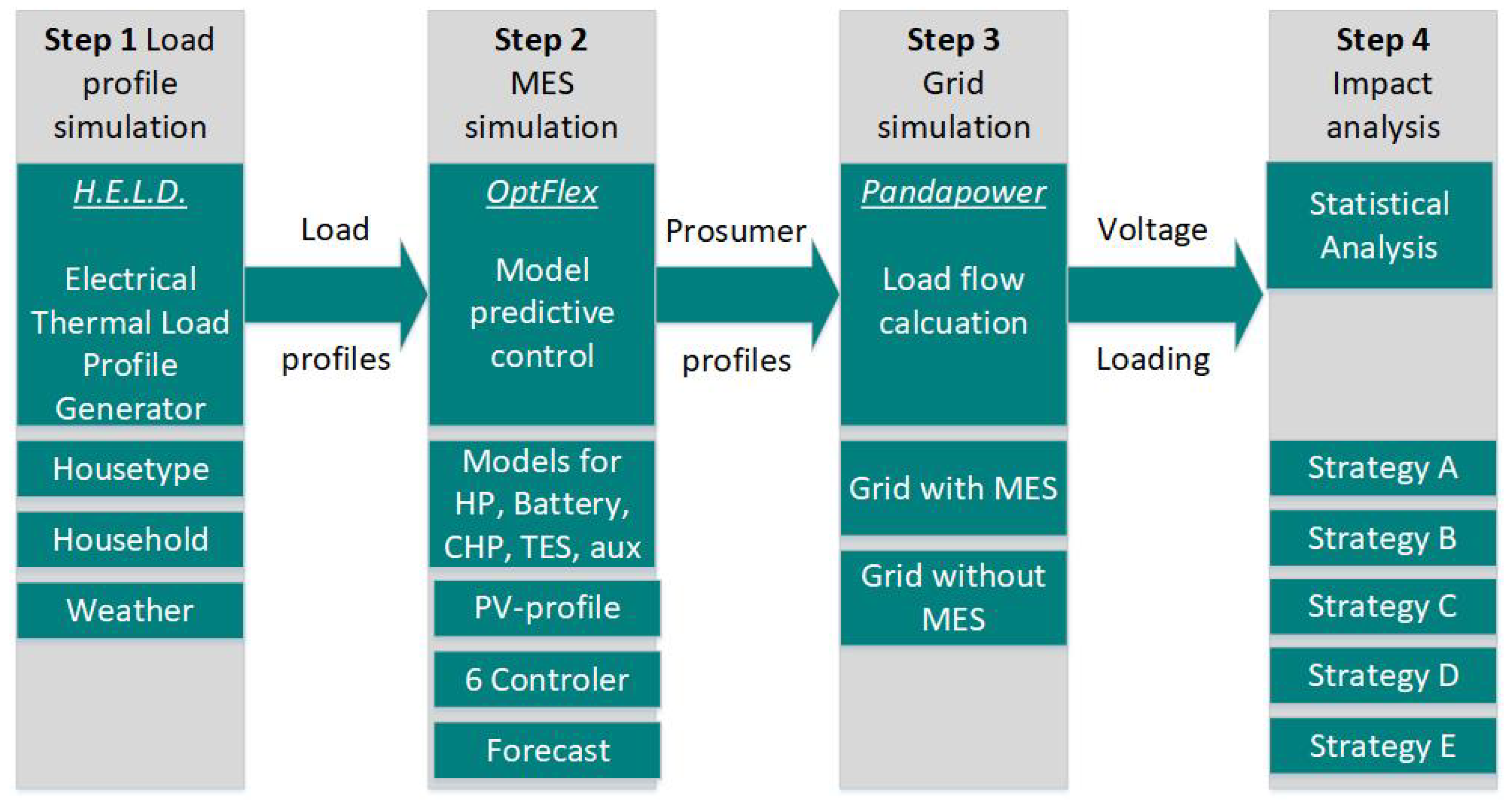
2.2. Step 2: MES Simulation (OptFlex)

Residential standard load profiles are commonly utilized directly as input for time-series-based power grid simulations and grid expansion planning. However, this assumption holds true only when no intelligent MESs are employed to optimize the energy supply within the household.

The OptFlex framework was developed in anticipation of a future where most households are equipped with MESs featuring intelligent controls [27]. This model aims to simulate the grid profiles of different MES types with varying control algorithms. The method implemented in the OptFlex model involves an optimized Model Predictive Control (MPC) algorithm based on a mixed-integer linear problem (MILP). This algorithm calculates time schedules for each component of the MES for the next 6 h (prediction horizon). The initial values of these time schedules are then used as set points for the components. The MPC is realized with two distinct cost functions: minimizing operational costs and minimizing CO₂ emissions [28].

Three different types of MESs are modeled with distinct control approaches:

• PV-Battery Systems:

One of these consists of a lithium-ion battery and a photovoltaic (PV) system. Note: PV-battery systems do not typically qualify as MESs since they lack thermal components. However, in our model, I assumed that PV-battery houses are equipped with oil or gas burners, which are independently controlled and therefore not explicitly modeled here.

• PV-HP Systems

One of these consists of a lithium-ion battery, a heat pump (HP), a thermal storage, and an electrical heater.

• PV-CHP Systems

One of these consists of a lithium-ion battery, a combined heat and power (CHP) plant, a thermal storage, and a gas boiler.

It is important to note that while PV-battery systems do not inherently include thermal components, our model assumes the presence of oil or gas burners in PV-battery houses. These burners are independently controlled and were thus not explicitly modeled here. The addition of the PV battery system to our impact analysis will help us calculate the impact of additional heating systems compared to pure electricity prosumers.

The objective function $J_{cost}\left(k\right)$ of the cost-MPC is formulated to achieve minimal operational costs. For the PV-CHP energy system, the function is presented by the following equation:

$$\begin{array}{ccc}\hfill J_{\mathrm{cost},\mathrm{CHP}}\left(k\right)& =& \sum _{j=k}^{{\mathrm{N}}_{\mathrm{p}}+\mathrm{k}}{C}_{\mathrm{gas}}·E_{\mathrm{gas},j}^{\mathrm{CHP}}\left(k\right)+C_{\mathrm{gas}}·E_{\mathrm{gas},j}^{\mathrm{boiler}}\left(k\right)+C_{\mathrm{el}}·E_{\mathrm{imp},j}^{\mathrm{grid}}\left(k\right)\hfill \\ \hfill & +& c_{\mathrm{up}}^{\mathrm{CHP}}·b_{\mathrm{up},j}^{\mathrm{CHP}}\left(k\right)+C_{\mathrm{FIT}}^{\mathrm{CHP}}·E_{\exp ,j}^{\mathrm{CHP}}\left(k\right)+C_{\mathrm{sc}}^{\mathrm{CHP}}·E_{\mathrm{sc},j}^{\mathrm{CHP}}\left(k\right)+C_{\mathrm{FIT}}^{\mathrm{PV}}·E_{\exp ,j}^{\mathrm{PV}}\left(k\right)\hfill \end{array}$$

(1)

with $N_{\mathrm{p}}$ as the prediction horizon; $C_{\mathrm{gas}}$, the gas cost; $C_{\mathrm{el}}$, the electricity cost; $c_{\mathrm{up}}^{\mathrm{CHP}}$, the CHP cold start costs; $C_{\mathrm{FIT}}^{\mathrm{CHP}}$, the feed-in tariff for CHP-generated electricity; $C_{\mathrm{FIT}}^{\mathrm{PV}}$, the feed-in tariff for PV-generated electricity; $C_{\mathrm{sc}}^{\mathrm{CHP}}$, the self-consumption; $E_{\mathrm{gas},j}^{\mathrm{CHP}}\left(k\right)$, the energy produced by the CHP; $E_{\mathrm{gas},j}^{\mathrm{boiler}}\left(k\right)$, the energy produced by the gas boiler; $E_{\mathrm{imp},j}^{\mathrm{grid}}\left(k\right)$, the energy imported from the grid; $b_{\mathrm{up},j}^{\mathrm{CHP}}\left(k\right)$, the binary variable used to turn the CHP plant on and off; $E_{\exp ,j}^{\mathrm{CHP}}\left(k\right)$, the energy produced by the CHP plant and exported to the grid; $E_{\mathrm{sc},j}^{\mathrm{CHP}}\left(k\right)$, the energy produced by the CHP plant and consumed directly by the household load; and $E_{\exp ,j}^{\mathrm{PV}}\left(k\right)$, the energy produced by the PV systems and exported to the grid. The calculation is processed for each time step k of the studied time period, such as one day or one year.

The objective function for the PV-HP systems is formulated as

$$\begin{array}{ccc}\hfill J_{\mathrm{cost},\mathrm{HP}}\left(k\right)& =& \sum _{j=k}^{{\mathrm{N}}_{\mathrm{p}}+\mathrm{k}}{C}_{\mathrm{el}}·E_{\mathrm{imp},j}^{\mathrm{grid}}\left(k\right)-C_{\mathrm{FIT}}^{\mathrm{PV}}·E_{\exp ,j}^{\mathrm{PV}}\left(k\right)\hfill \end{array}$$

(2)

The objective function for the PV-battery systems is the same equation as for the PV-HP system, formulated as:

$$\begin{array}{ccc}\hfill J_{\mathrm{cost},\mathrm{batt}}\left(k\right)& =& \sum _{j=k}^{{\mathrm{N}}_{\mathrm{p}}+\mathrm{k}}{C}_{\mathrm{el}}·E_{\mathrm{imp},j}^{\mathrm{grid}}\left(k\right)-C_{\mathrm{FIT}}^{\mathrm{PV}}·E_{\exp ,j}^{\mathrm{PV}}\left(k\right)\hfill \end{array}$$

(3)

If not specified otherwise, the costs are set at EUR 0.0652 for natural gas and EUR 0.2838 for electricity. The feed-in tariffs are EUR 0.1256 for PV and EUR 0.09392 for CHP. Moreover, for the CHP system, a cold start cost of EUR 0.02 Euro is considered, and energy provided by the CHP, which is consumed within the household, is reimbursed with EUR 0.005.

The objective function $J_{C{O}_2}\left(k\right)$ of the Model Predictive Control (MPC) is formulated to achieve minimal CO₂ production. The following equations present the function:

$$\begin{array}{ccc}\hfill J_{{\mathrm{CO}}_2,\mathrm{CHP}}\left(k\right)& =& \sum _{j=k}^{{\mathrm{N}}_{\mathrm{p}}+\mathrm{k}}{e}_{\mathrm{gas}}^{{\mathrm{CO}}_2}·E_{\mathrm{gas},j}^{\mathrm{aux}}\left(k\right)+{ϵ}_{\mathrm{gas}}^{{\mathrm{CO}}_2}·E_{\mathrm{gas},j}^{\mathrm{CHP}}\left(k\right)+{ϵ}_{\mathrm{grid}}^{{\mathrm{CO}}_2}·E_{\mathrm{imp},j}^{\mathrm{grid}}\left(k\right)\hfill \\ \hfill & +& {ϵ}_{\mathrm{PV}}^{{\mathrm{CO}}_2}·E_{\exp ,j}^{\mathrm{PV}}\left(k\right)+{ϵ}_{\mathrm{PV}}^{{\mathrm{CO}}_2}·E_{\mathrm{batt},j}^{\mathrm{PV}}\left(k\right)+{ϵ}_{\mathrm{PV}}^{{\mathrm{CO}}_2}·E_{\mathrm{load},j}^{\mathrm{PV}}\left(k\right)\hfill \end{array}$$

(4)

where $N_{\mathrm{p}}$ is the prediction horizon, ${ϵ}_{\mathrm{gas}}^{{\mathrm{CO}}_2}$ is the emission coefficient of natural gas, ${ϵ}_{\mathrm{grid}}^{{\mathrm{CO}}_2}$ is the emission coefficient of the Germany electricity mix, ${ϵ}_{\mathrm{PV}}^{{\mathrm{CO}}_2}$ is the emission coefficient of PV energy, $E_{\mathrm{gas}}^{\mathrm{aux}}$ is the energy provided by the gas boiler, $E_{\mathrm{gas},j}^{\mathrm{CHP}}\left(k\right)$ is the energy provided by the CHP, $E_{\mathrm{imp},j}^{\mathrm{grid}}\left(k\right)$ is the energy provided by the grid, $E_{\exp ,j}^{\mathrm{PV}}\left(k\right)$ is the energy exported to the grid, $E_{\mathrm{batt},j}^{\mathrm{PV}}\left(k\right)$ is the energy charged into the battery; and $E_{\mathrm{load},j}^{\mathrm{PV}}\left(k\right)$ is the energy directly consumed by the household load.

The objective function for the PV-HP energy systems is formulated as

$$\begin{array}{ccc}\hfill J_{{\mathrm{CO}}_2,\mathrm{HP}}\left(k\right)& =& \sum _{j=k}^{{\mathrm{N}}_{\mathrm{p}}+\mathrm{k}}{ϵ}_{\mathrm{grid}}^{{\mathrm{CO}}_2}·E_{\mathrm{imp},j}^{\mathrm{grid}}\left(k\right)+{ϵ}_{\mathrm{PV}}^{{\mathrm{CO}}_2}·E_{\mathrm{eheat},j}^{\mathrm{PV}}\left(k\right)+{ϵ}_{\mathrm{PV}}^{{\mathrm{CO}}_2}·E_{\mathrm{HP},j}^{\mathrm{PV}}\left(k\right)\hfill \\ \hfill & +& {ϵ}_{\mathrm{PV}}^{{\mathrm{CO}}_2}·E_{\exp ,j}^{\mathrm{PV}}\left(k\right)+{ϵ}_{\mathrm{PV}}^{{\mathrm{CO}}_2}·E_{\mathrm{batt},j}^{\mathrm{PV}}\left(k\right)+{ϵ}_{\mathrm{PV}}^{{\mathrm{CO}}_2}·E_{\mathrm{load},j}^{\mathrm{PV}}\left(k\right)\hfill \end{array}$$

(5)

where $N_{\mathrm{p}}$ is the prediction horizon, ${ϵ}_{\mathrm{grid}}^{{\mathrm{CO}}_2}$ is the emission coefficient of the Germany electricity mix, ${ϵ}_{\mathrm{PV}}^{{\mathrm{CO}}_2}$ is the emission coefficient of the PV energy, $E_{\mathrm{imp},j}^{\mathrm{grid}}\left(k\right)$ is the energy provided by the grid, $E_{\mathrm{eheat},j}^{\mathrm{PV}}\left(k\right)$ is the PV energy consumed by the electrical heater, $E_{\mathrm{eheat},j}^{\mathrm{PV}}\left(k\right)$ is the PV energy consumed by the HP, $E_{\exp ,j}^{\mathrm{PV}}\left(k\right)$ is the energy exported to the grid, $E_{\mathrm{batt},j}^{\mathrm{PV}}\left(k\right)$ is the energy charged into the battery; and $E_{\mathrm{load},j}^{\mathrm{PV}}\left(k\right)$ is the energy directly consumed by the household load.

The objective function for the PV-battery systems is formulated as

$$\begin{array}{ccc}\hfill J_{{\mathrm{CO}}_2,\mathrm{batt}}\left(k\right)& =& \sum _{j=k}^{{\mathrm{N}}_{\mathrm{p}}+\mathrm{k}}{ϵ}_{\mathrm{grid}}^{{\mathrm{CO}}_2}·E_{\mathrm{imp},j}^{\mathrm{grid}}\left(k\right)+{ϵ}_{\mathrm{PV}}^{{\mathrm{CO}}_2}·E_{\exp ,j}^{\mathrm{PV}}\left(k\right)+{ϵ}_{\mathrm{PV}}^{{\mathrm{CO}}_2}·E_{\mathrm{batt},j}^{\mathrm{PV}}\left(k\right)\hfill \\ \hfill & +& {ϵ}_{\mathrm{PV}}^{{\mathrm{CO}}_2}·E_{\mathrm{load},j}^{\mathrm{PV}}\left(k\right)\hfill \end{array}$$

(6)

where $N_{\mathrm{p}}$ is the prediction horizon, ${ϵ}_{\mathrm{grid}}^{{\mathrm{CO}}_2}$ is the emission coefficient of the Germany electricity mix, $E_{\mathrm{imp},j}^{\mathrm{grid}}\left(k\right)$ is the energy provided by the grid, ${ϵ}_{\mathrm{PV}}^{{\mathrm{CO}}_2}$ is the emission coefficient of the PV energy, $E_{\exp ,j}^{\mathrm{PV}}\left(k\right)$ is the energy of the PV system exported to the grid, $E_{\mathrm{batt},j}^{\mathrm{PV}}\left(k\right)$ is the energy charged into the battery, and $E_{\mathrm{load},j}^{\mathrm{PV}}\left(k\right)$ is the energy directly consumed by the household load.

The emission coefficients were chosen to be 587 g/kWh for the German electricity mix, 202 g/kWh for natural gas, and 0 g/kWh for PV-generated energy.

Additional constraints, including the electrical and thermal energy balance, are necessary to evaluate the objective functions. Detailed constraints and a comprehensive parameter description can be found in the Appendix of [27,28,29] and in Appendix B of this paper. The optimization problem is solved using Pyomo 5.7.2 [30,31] with a CPLEX solver by IBM (Armonk, NY, USA).

The output time profiles obtained from the previous section are utilized as input for the MES control algorithm. Time profiles for the energy system parameters, including profiles at the MES’s grid connection points, are then calculated. In total, 12 optimized PV-Battery systems, 7 optimized PV-HP systems, and 4 optimized PV-CHP systems were modeled. The number of systems corresponds to the number of buses in the distribution grid feeder in the subsequent section.

The MES simulation using the OptFlex framework was conducted for the following control strategies, motivated by [29]. The assumptions are also summarized in

Table 3. Overview of assumed parameters for control strategies.

	Strategy A	Strategy B	Strategy C	Strategy D	Strategy E
MES placement: basic/test grid	fixed/fixed	fixed/fixed	fixed/fixed	fixed/fixed	fixed/random
Feed-in tariffs	on	off	off	off	on
Electrictiy price	const.	EEX	const.	const.	const.
Cost function	OPEX	OPEX	CO2	OPEX	OPEX
Forecast	perfect	perfect	perfect	perfect	perfect
Peak shaving	off	off	off	off	off

:

• Strategy A: “Feed-In incentives”

The MPC control is optimized for operational costs, assuming constant electricity costs. The parameters for feed-in incentives and other factors are set as follows: natural gas, EUR 0.0652; electricity, EUR 0.2838; feed-in tariff for PV, EUR 0.1256; feed-in tariff for CHP, EUR 0.09392; cold-start cost for CHP, EUR 0.02; and reimbursement for energy provided by CHP consumed within the household, EUR 0.005.

• Strategy B: “Without incentives”

The MPC control is optimized for operational costs, with constant electricity costs assumed. A perfect forecast method is selected. No feed-in incentives are assumed; hence, the PV and CHP feed-in tariff and self-consumption reimbursement are set to zero. The cost for the cold start of the CHP and the electricity/gas costs are chosen as in Strategy A.

• Strategy C: “CO₂ reduction”

The MPC control is optimized for minimal CO₂ emission, with emission coefficients set as follows: 587 g/kWh for the German electricity mix, 202 g/kWh for natural gas, and 0 g/kWh for PV-generated energy. Constant electricity costs are assumed. The forecast method is chosen to be perfect forecast. No other feed-in incentives are assumed and are set to zero as in Strategy B.

• Strategy D “Market oriented”

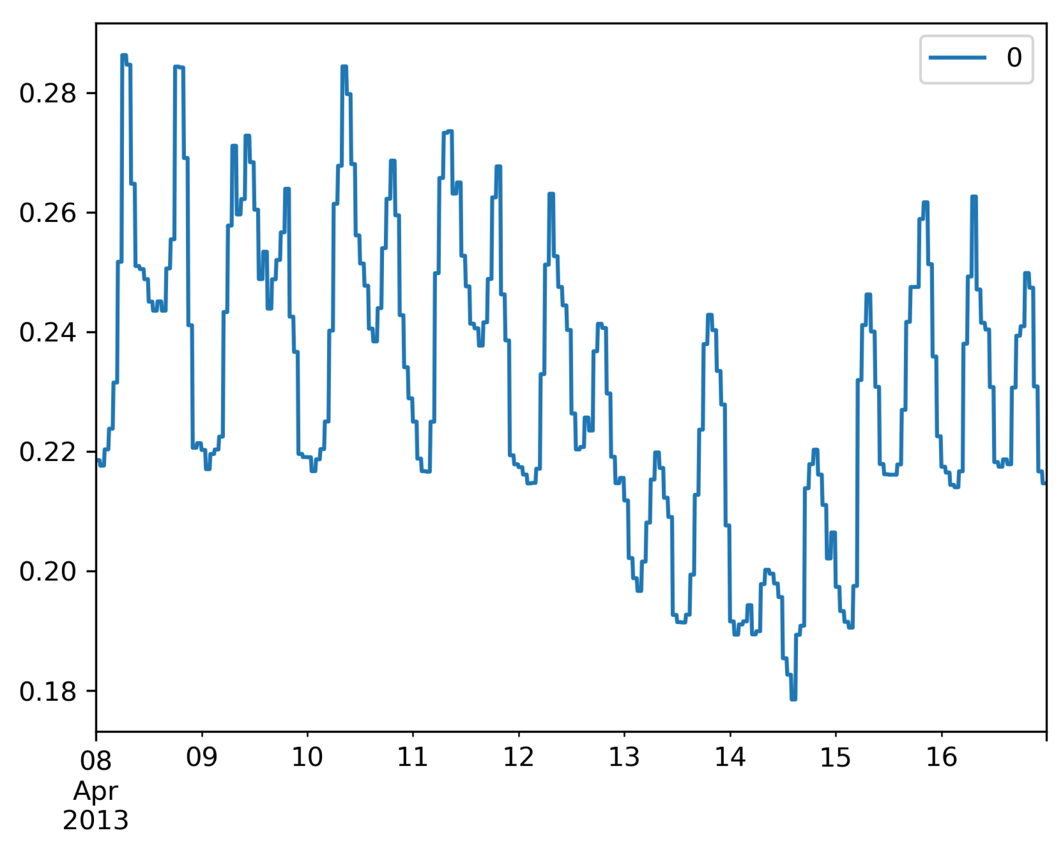
The MPC control is optimized for operational costs, with time-dependent electricity prices assumed. An example is illustrated in Figure 3. No other feed-in incentives are assumed and are set to zero as in Strategies B and C.

• Strategy E “Random MES placement”

The MPC control strategy remains the same as in Strategy A. However, in this strategy, the placements of the different MESs are randomly chosen to study the effect of clustering.

• Grid Profiles

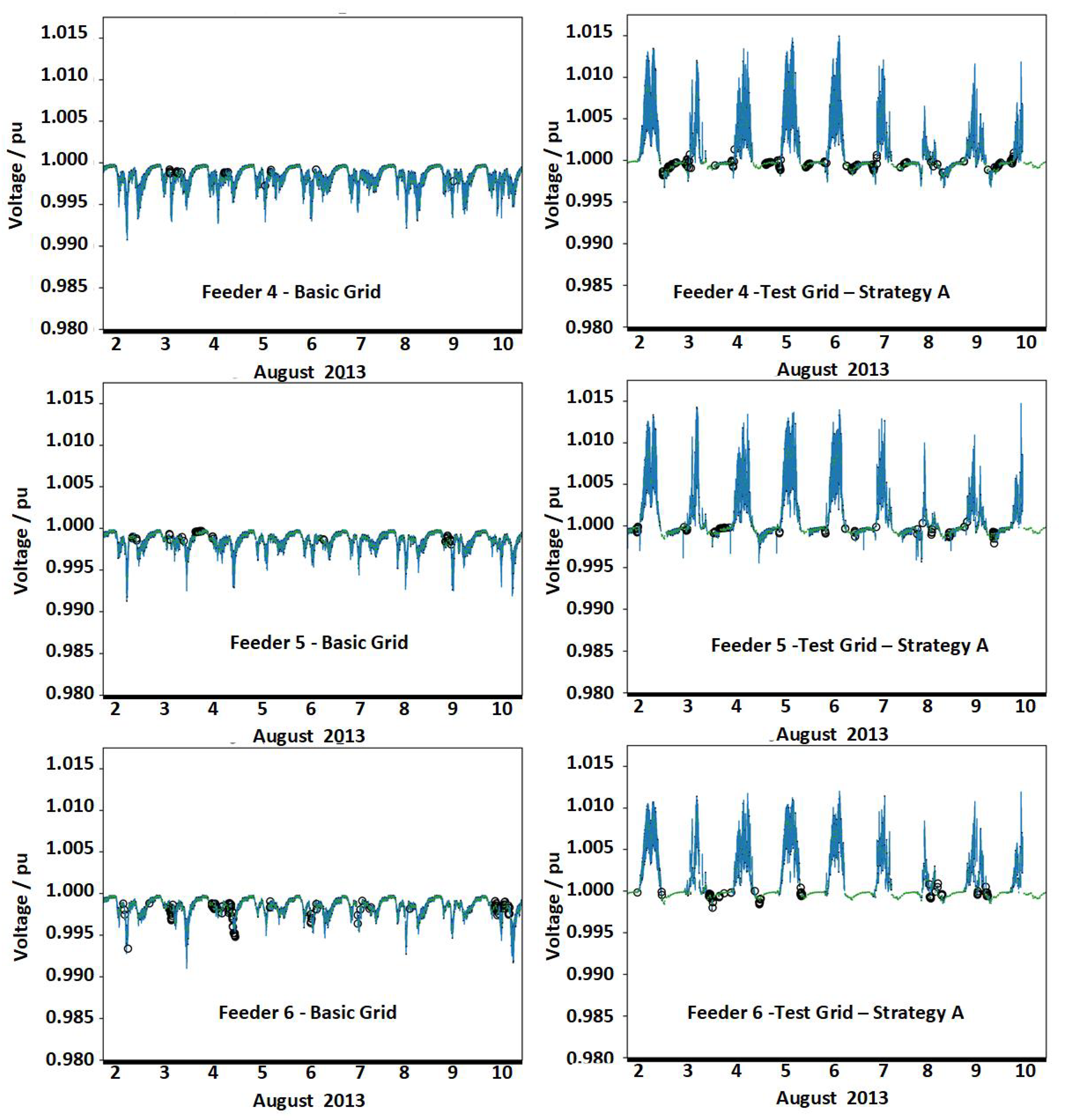
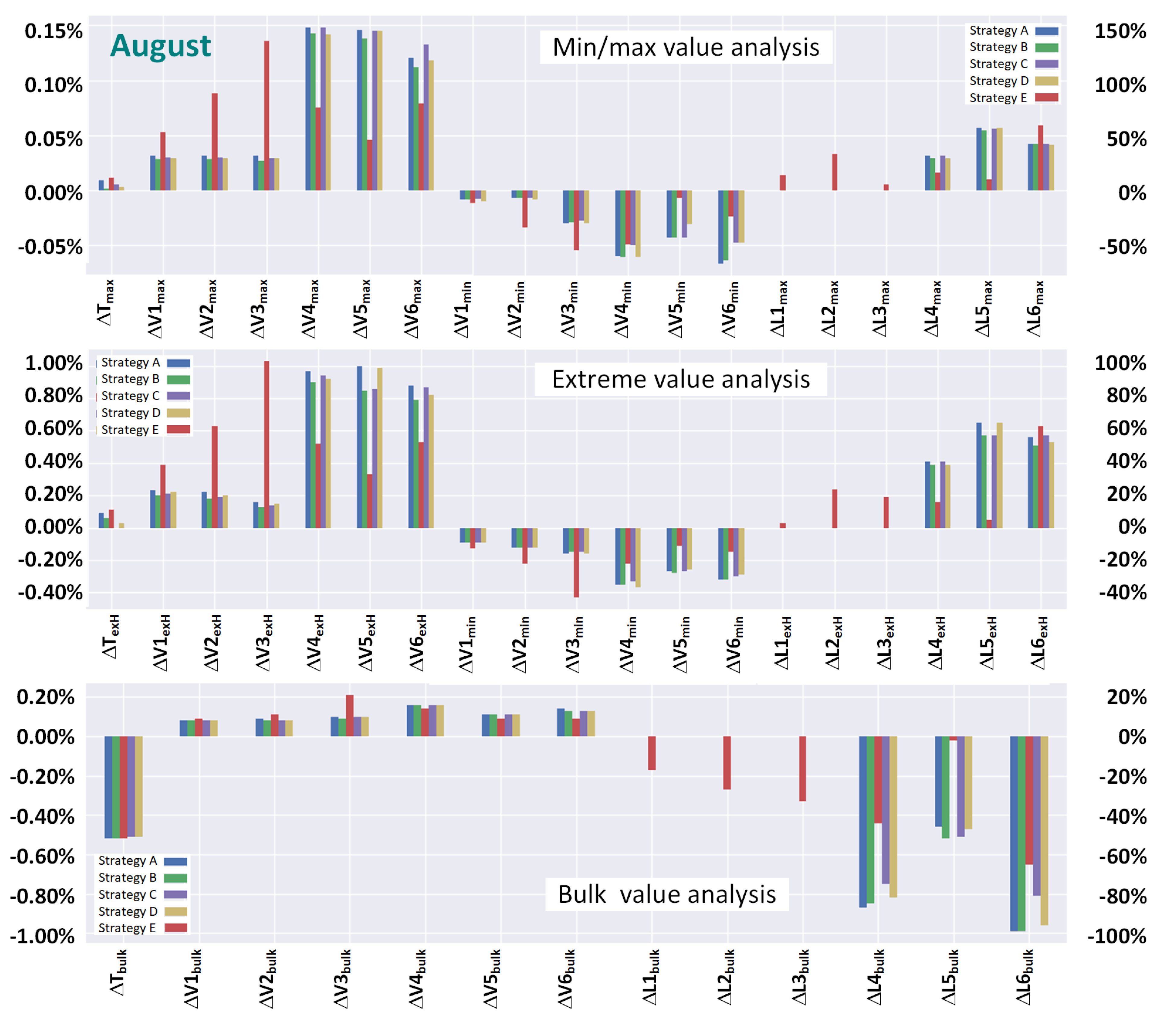
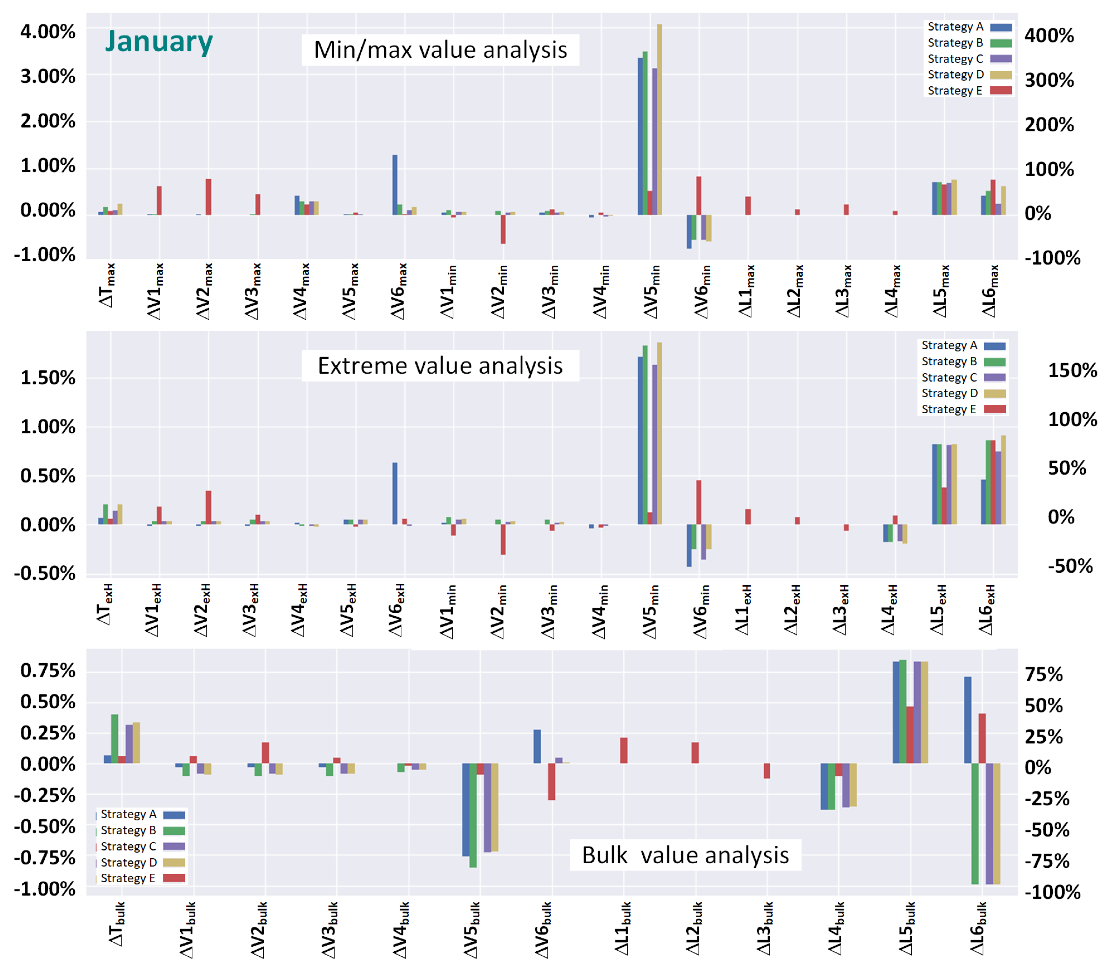
The OptFlex algorithm is utilized to produce the profiles at the MES’s grid connection points. Additionally, key performance indicators can be calculated to characterize the MES’s behavior for the different control strategies. For the studied grid, 12 optimized PV-Battery systems, 7 optimized PV-HP systems, and 4 optimized PV-CHP systems were modeled. The profiles can be computed for different time periods. Calculations up to one year were conducted for single-MES systems. Subsequently, nine days in August, nine days in January, and nine days in April, representing the summer, winter, and transition period seasons, were calculated. This method enables us to study different features and outcomes based on various seasonal effects, which is important since MESs also include heating devices exhibiting temperature-dependent behaviors. The calculations were performed for all five strategies described in the last section.

To gain an understanding of the results from this simulation step, I will showcase only one example for each MES type. I plotted profiles for the transition period, where features such as PV emission and all three energy demands (electrical, space heating, and domestic hot water) are present. In the summer, no space heating is needed, and in the winter, only small amounts of PV emission are present. The presence of all four input time profiles leads to interesting control decisions. The summer and winter period results are shown in the Appendix B in Figure A1 and Figure A2.

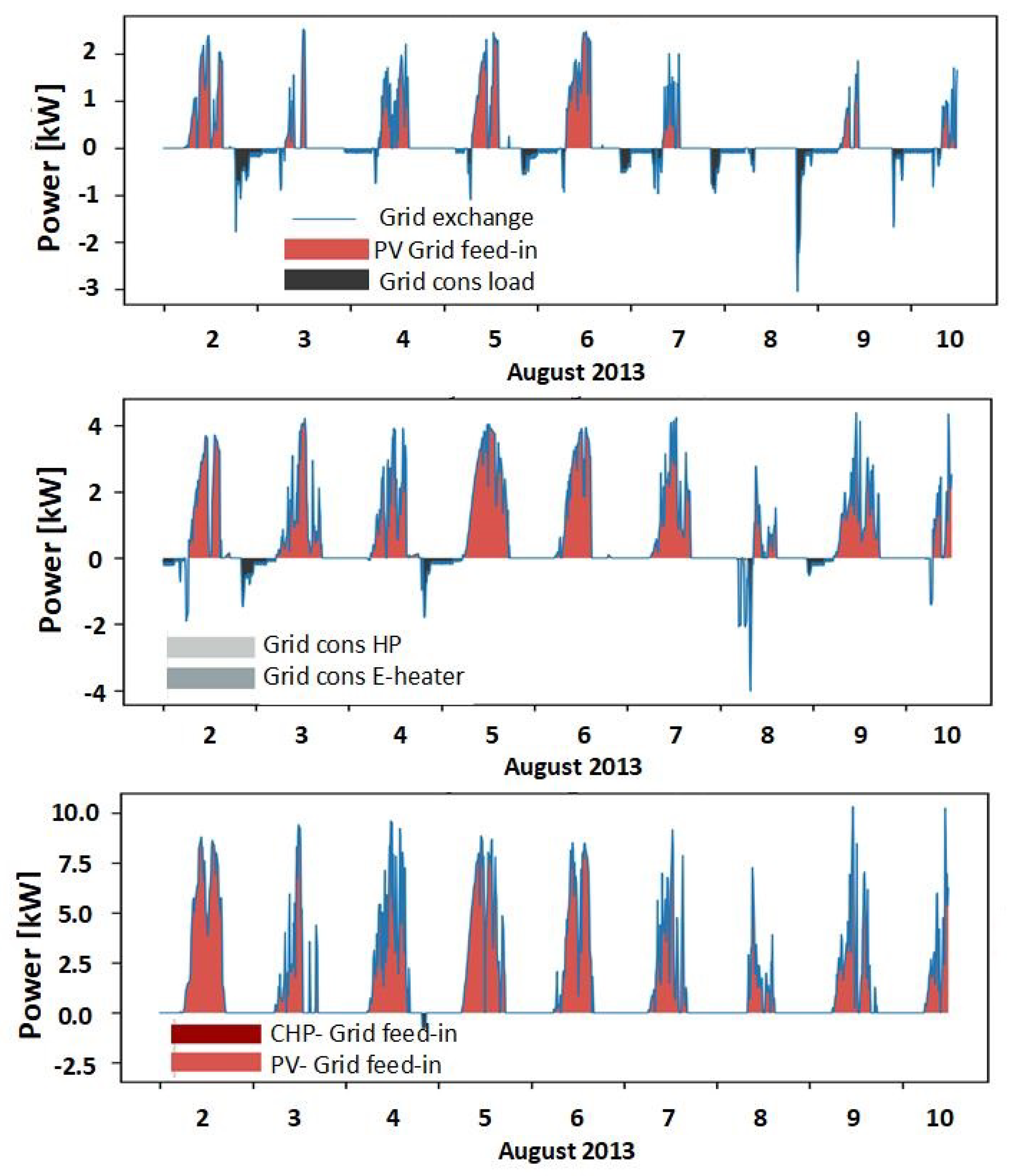
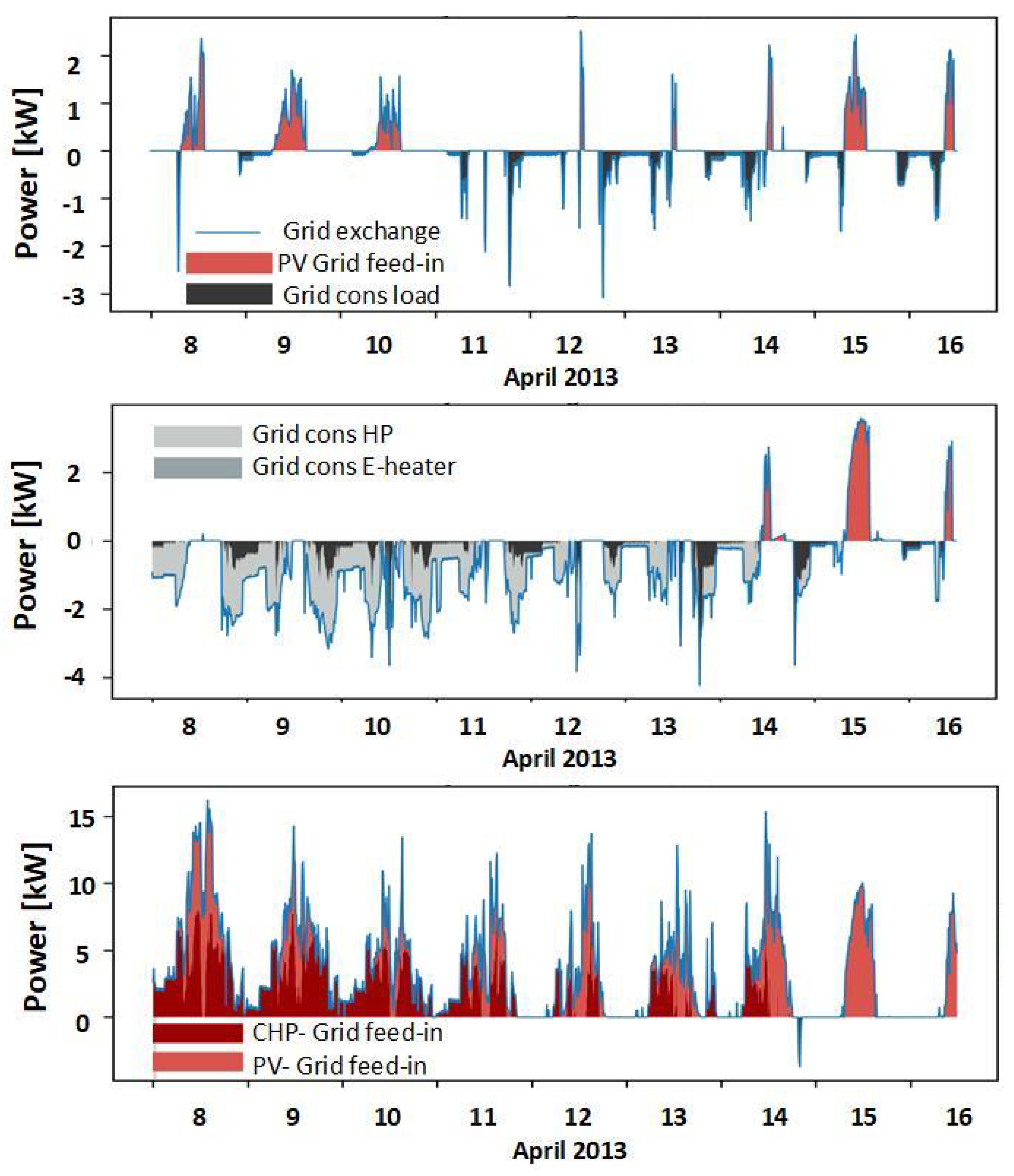
In Figure 4, profiles for Strategy A are displayed. The energy fed into the grid is plotted as positive values, while consumed energy is depicted with negative numbers. Each energy system exhibits distinct grid profiles.

• The PV-battery system (upper panel) displays the PV-grid feed (light red) and electricity consumption for the household load (black).
• The profile of a PV-HP system is characterized by electricity consumption from the grid to meet the demands of the household load (black), HP (light gray), and the electrical heater (dark grey), with a high PV self-consumption rate during the initial 6 days.
• The grid profile of the PV-CHP system is dominated by feed-in energy produced by the PV system (light red) and the CHP (dark red).

During the last three days, the PV-battery and PV-HP systems exhibit comparable behaviors. Initially, the battery is discharged to cover the household load, and then energy is drawn from the power grid. As soon as PV energy becomes available, it is used directly for the household load and the HP, while the surplus is stored in the battery. If insufficient PV energy is available, the battery is discharged. When the battery is depleted, grid consumption begins to cover the electrical loads. During these days, as the space-heating demand decreases due to rising outdoor temperatures, the behaviors of the PV-battery and PV-HP systems converge.

In contrast, the PV-CHP system demonstrates a completely different grid profile. No external energy is required from the grid. The CHP energy meets the electrical load, while all PV energy is fed into the grid. As the space-heating demand decreases during the last three days, the CHP operates less frequently, resulting in reduced feed-in energy production. This behavior is attributed to the assumptions of Strategy A, where incentives prioritize feeding PV and CHP energy into the grid.

2.3. Grid Simulation (Pandapower)

The distribution network utilized in the analysis was a standardized grid designed specifically for scientific investigation. Known as “Kerber networks,” these grids are derived from the distribution networks featured in the dissertation titled “Capacity of low voltage distribution networks with increased feed-in of photovoltaic power” by Georg Kerber. 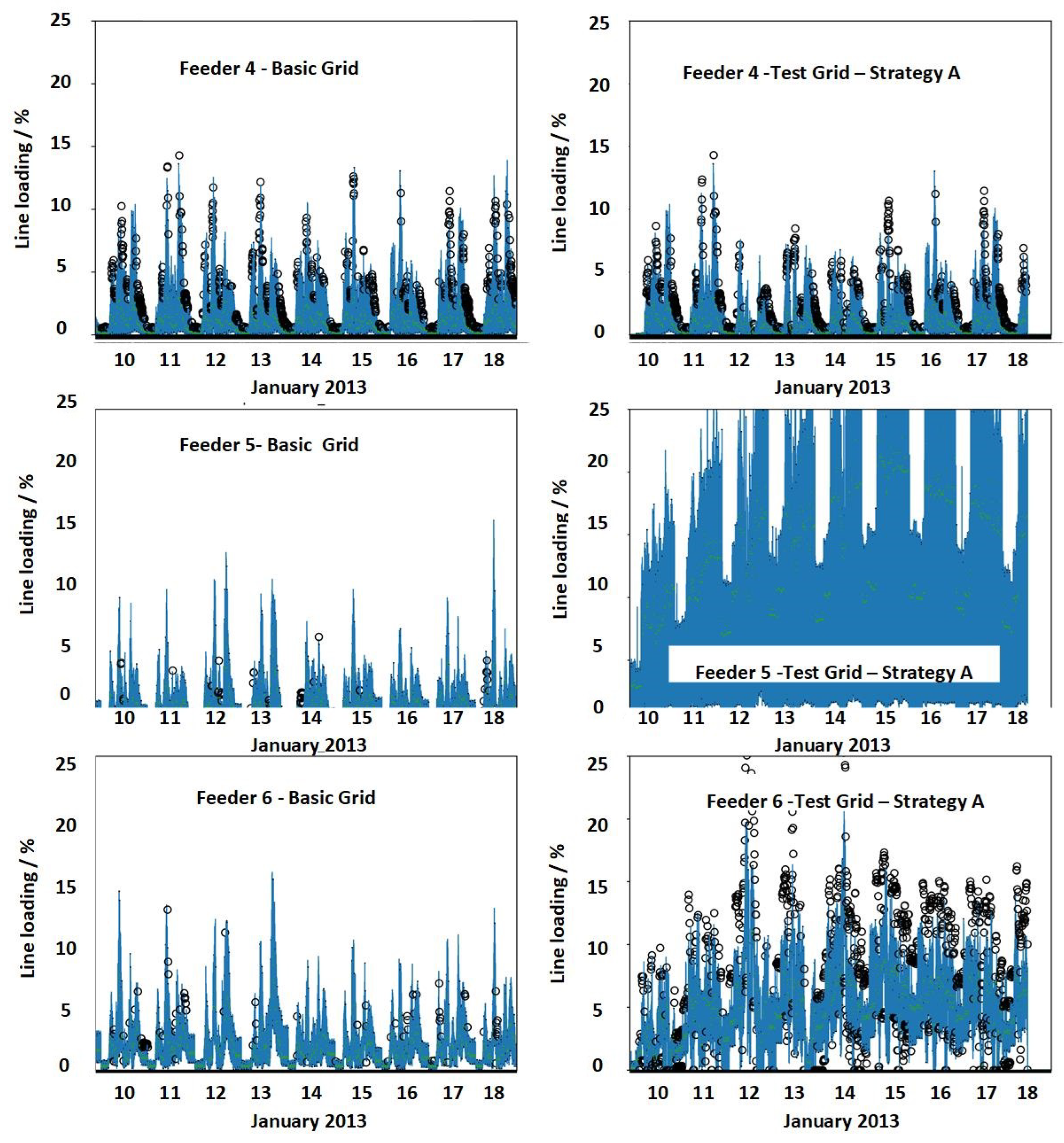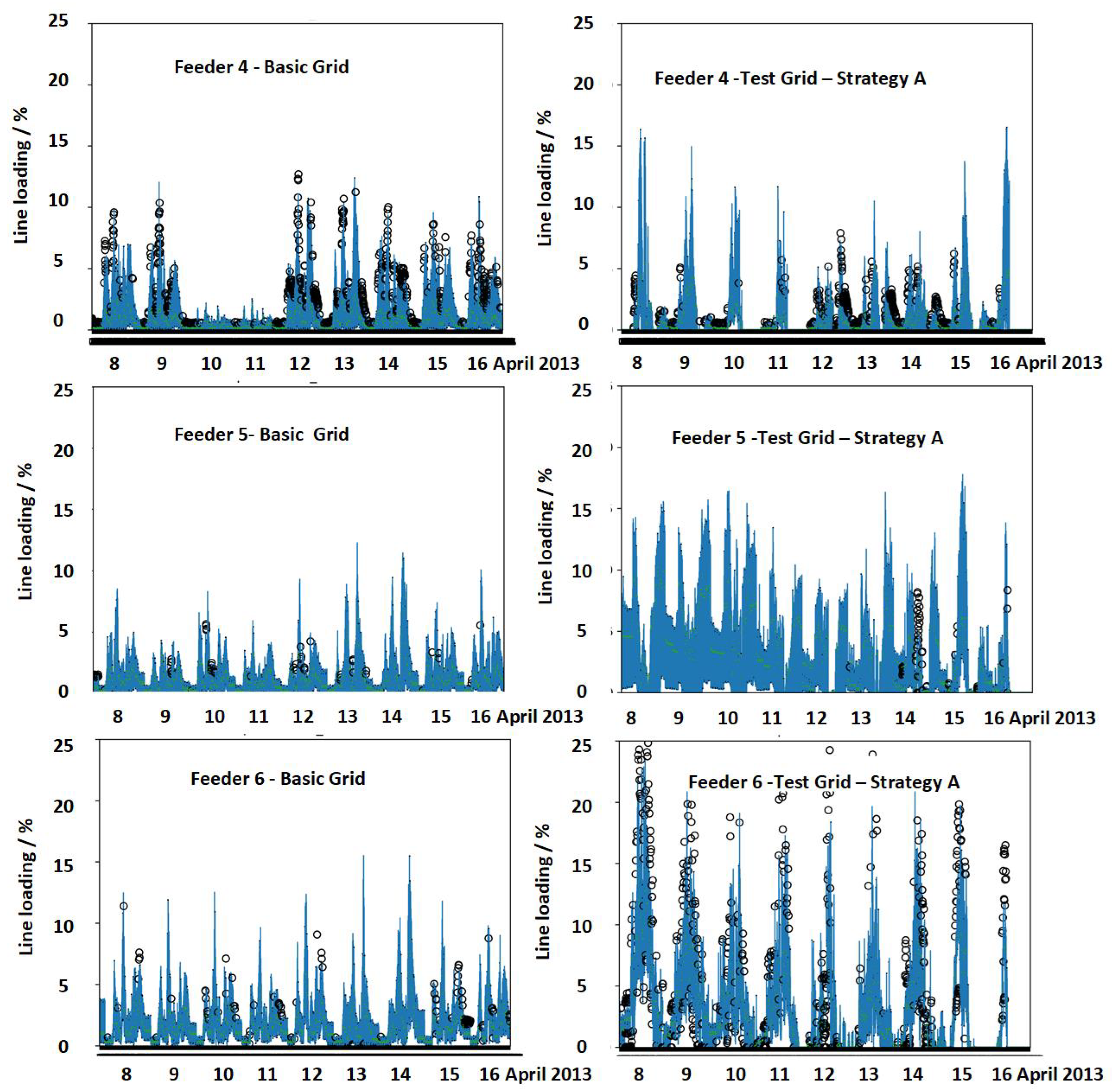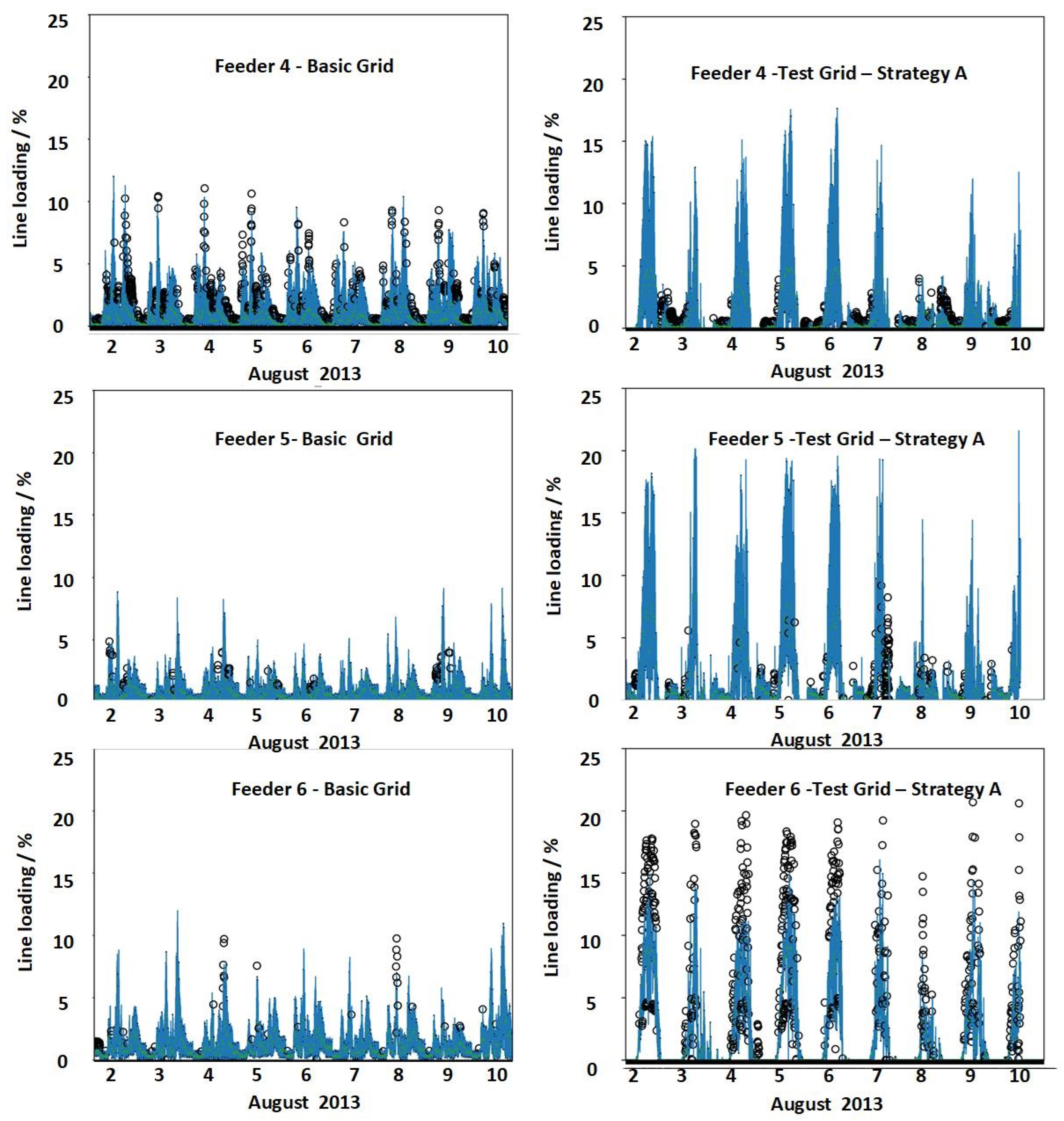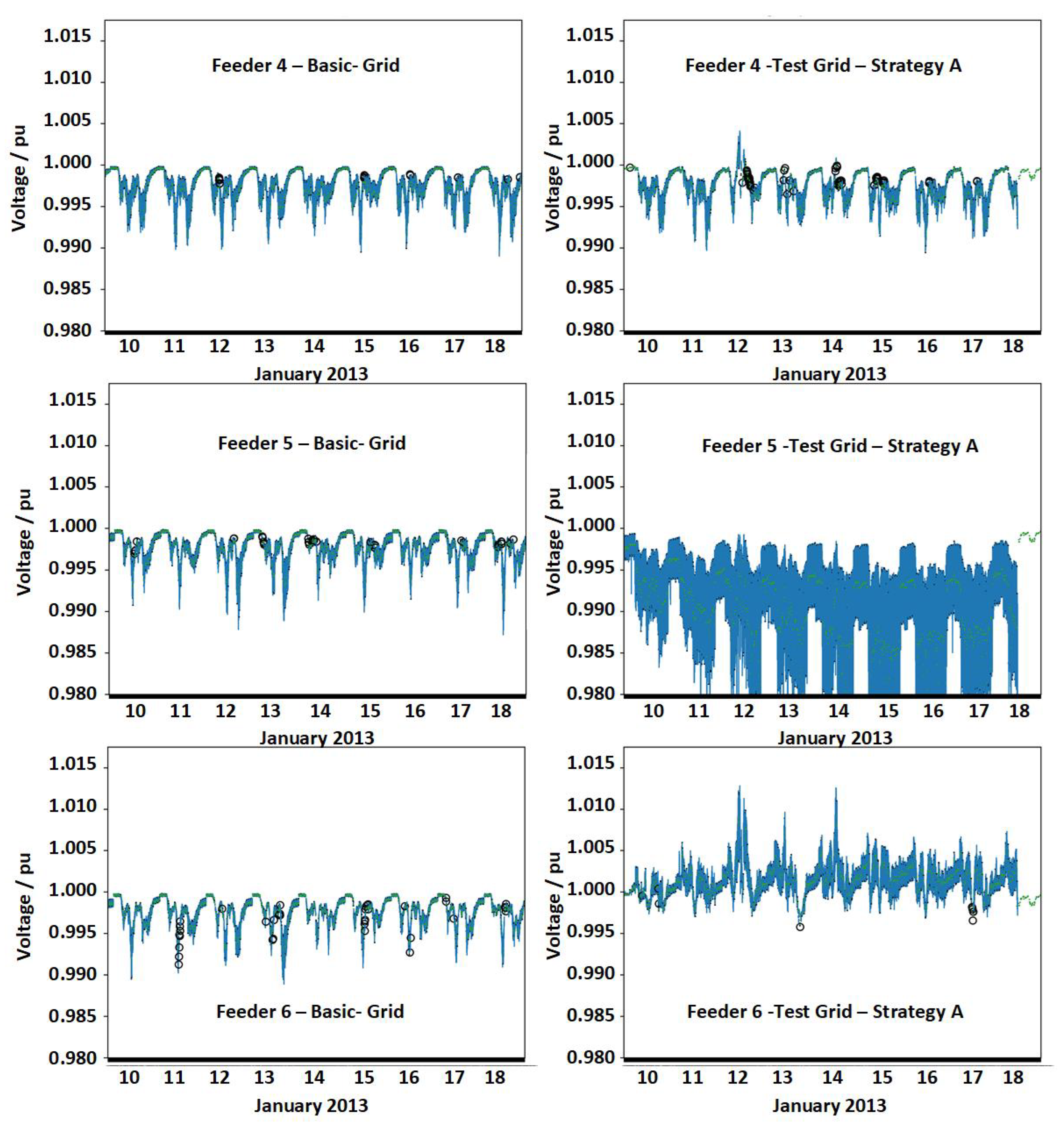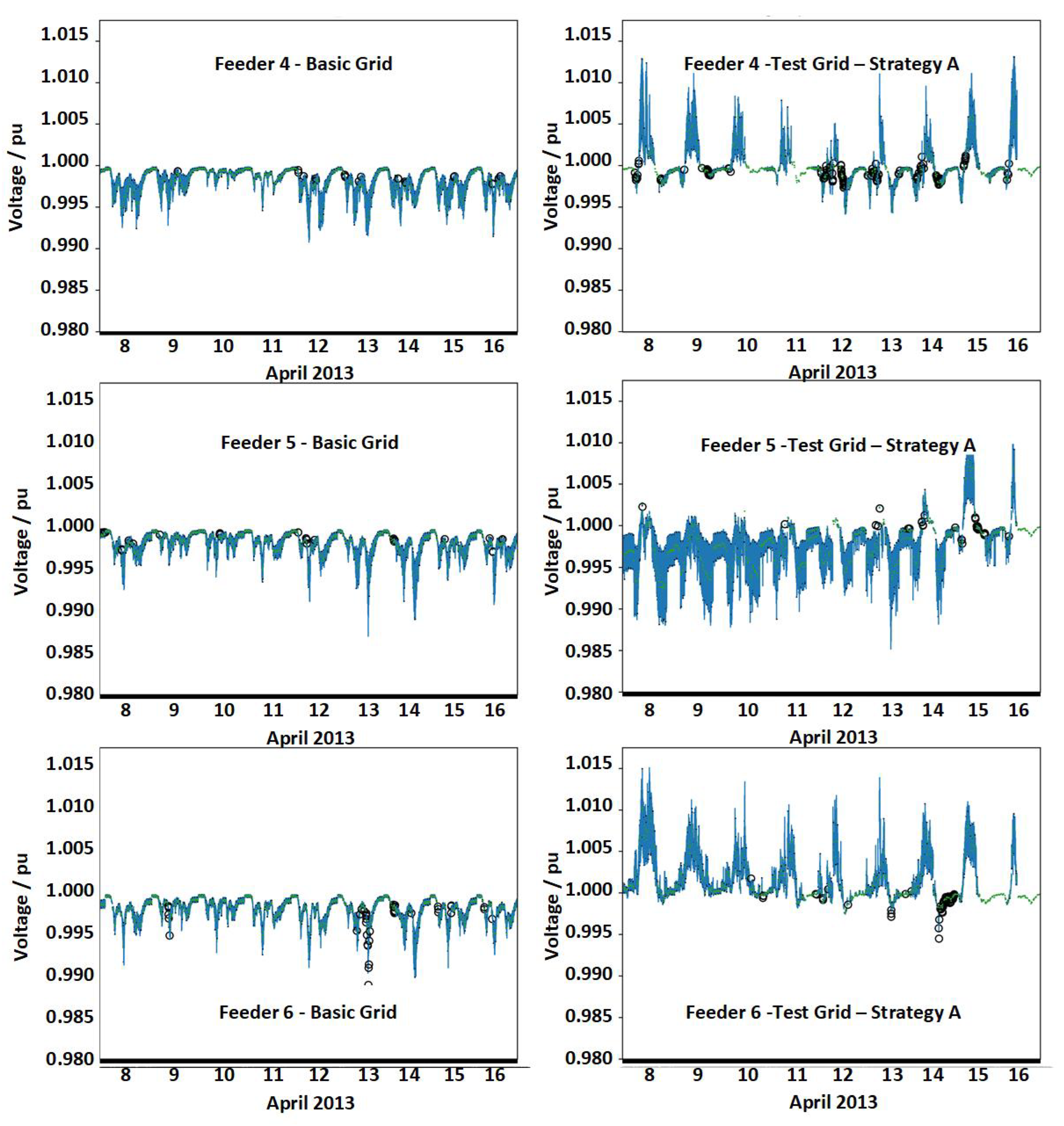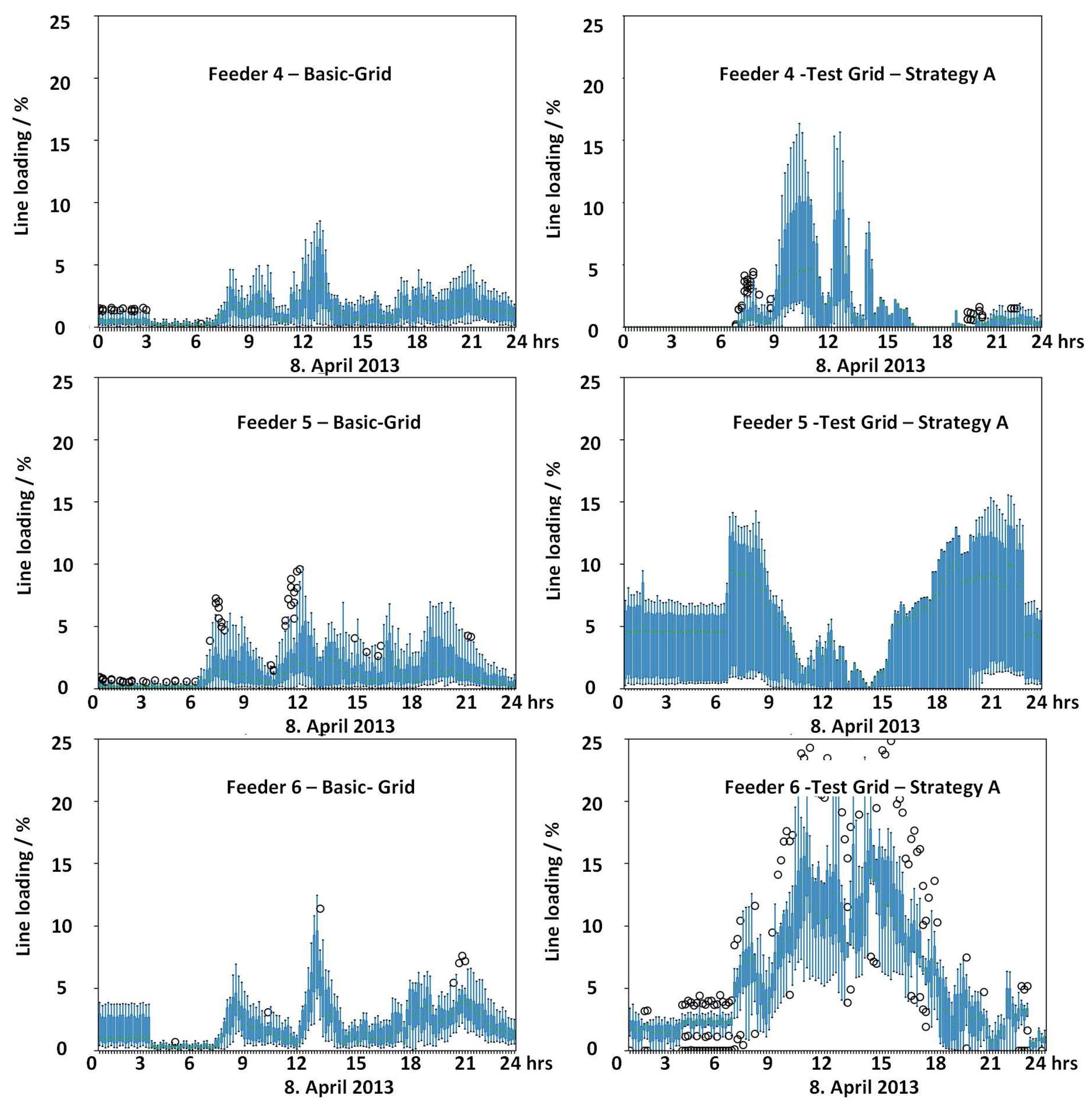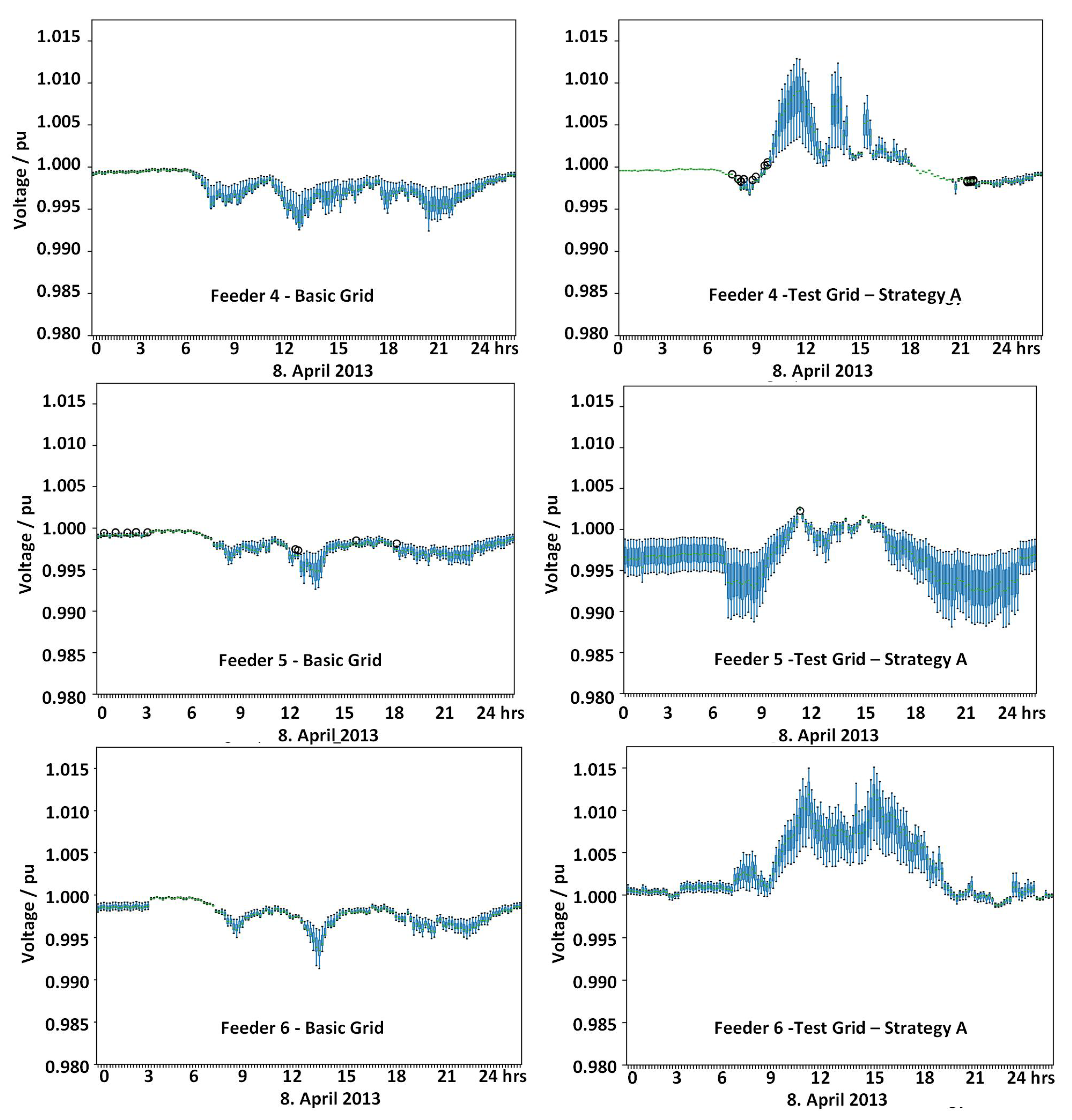(For reproducibility, please find the network data on the pandapower homepage: https://pandapower.readthedocs.io/en/latest/networks/kerber.html#average-kerber-networks, accessed on 21 June 2024) To examine the influence of various MES types, control strategies, and seasonal variations, the following methodology was employed. Initially, a “Basic-Grid” was established using a generic distribution grid. Subsequently, multiple “Test-Grids” were formulated, each incorporating different MES types and control strategies, all based on the same generic distribution grid. The impact of these control strategies and MES types was assessed in comparison to the “Basic-Grid.” It is important to note that the analysis did not extend to evaluating grid violations or planning for grid expansion. Instead, the aim was to identify general impact characteristics utilizing a generic grid model, without delving into specific grid violation analyses, which are heavily reliant on real grid model parameters and assumed grid violation limits.

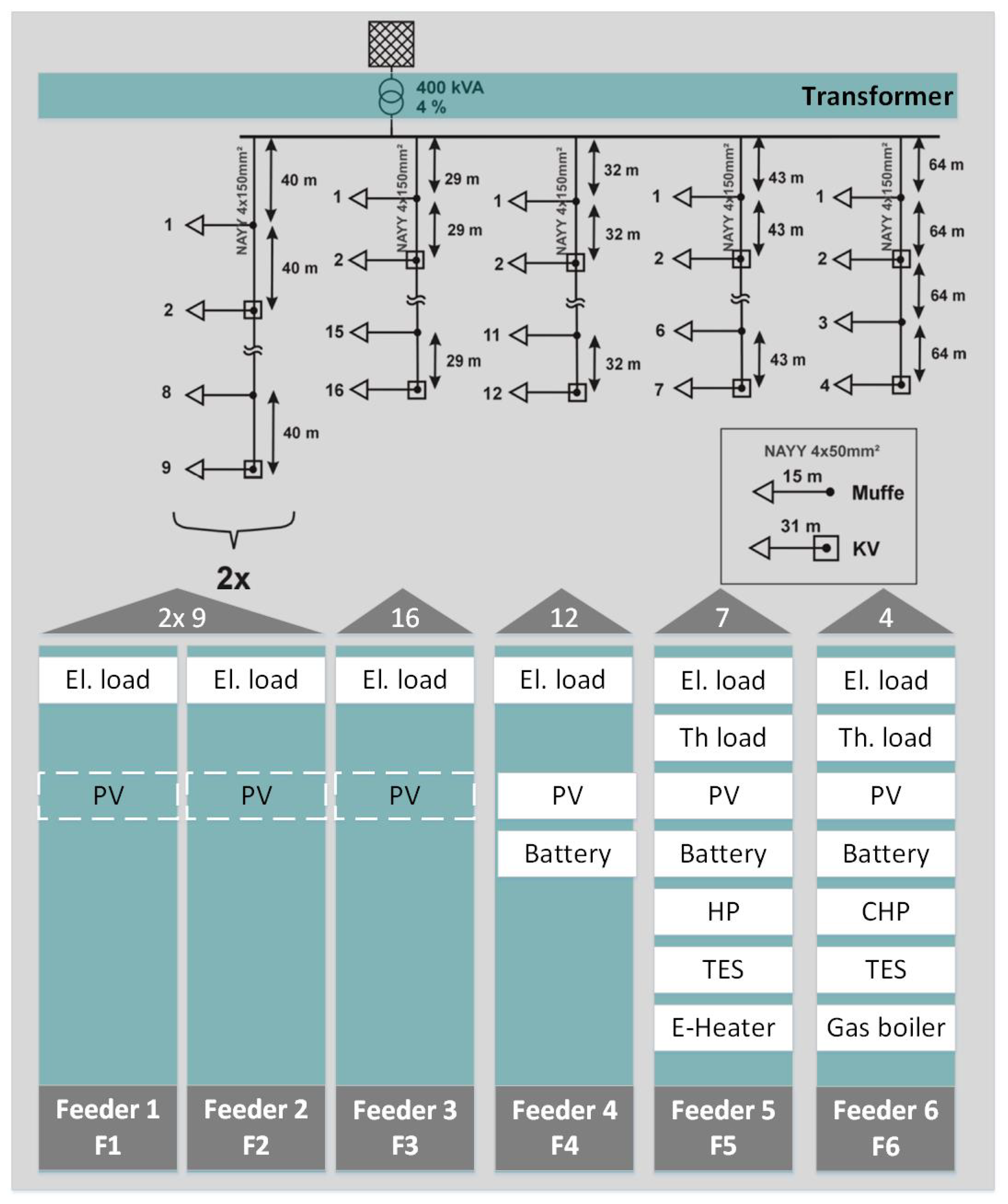
To create a realistic urban environment, I needed to integrate the MES with the load busses of the distribution grid, forming a small section of a generic city. The grid comprises six feeders, with feeder 1 to feeder 3 representing areas where conventional energy systems and decentralized PV are not installed. On the other hand, feeder 4 to feeder 6 represent three distinct types of streets, as depicted in Figure 5. I assumed that each feeder has similar construction year classes and heating systems. Consequently, one feeder is linked to PV-battery systems, another feeder solely to PV-HP systems, and the remaining feeder exclusively to PV-CHP systems. This approach is aimed at simulating a significant impact on the grid due to the high simultaneity of MESs. Such configurations may mirror real scenarios in distribution grids and cities, where districts and streets often share ownership or are developed with similar energy concepts. Feeders 4–6 were configured as follows:

• Feeder 4: “PV-Battery systems”. I have 12 houses equipped with PV-battery systems, each with a separate heat supply, either through oil heating or the gas grid. These houses are predominantly single-family homes. The heat demand for these buildings is not explicitly defined (nd) and was set to a default value.
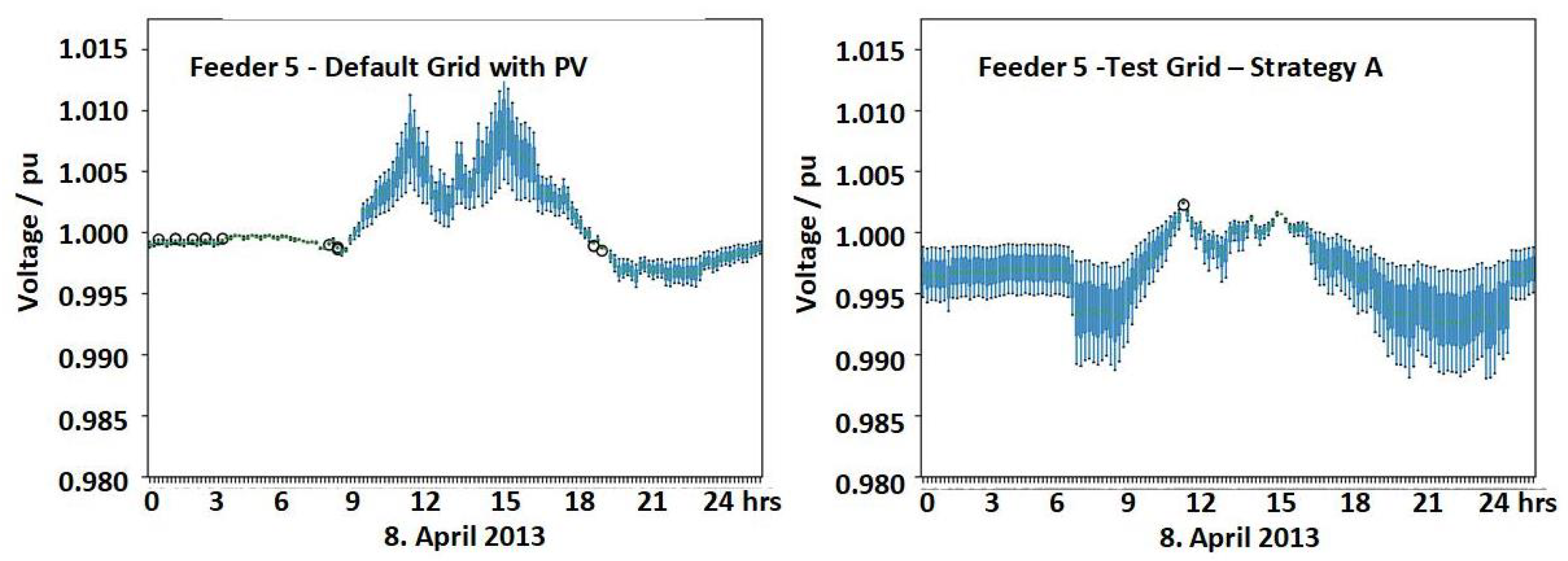
• Feeder 5: “PV-HP systems”. There are 7 new homes, primarily single-family dwellings, built in the years 2000, 2005, and 2010. These homes rely on the electrical grid for space heating and domestic hot water.
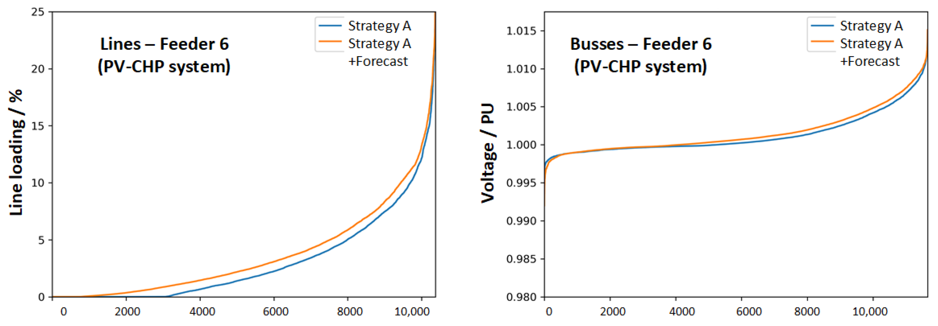
• Feeder 6: “PV-CHP systems”. There are four older multi-family homes where heating demand is solely provided by the gas grid.

The Basic-Grid is defined as the Kerber-grid, which was outfitted with randomly selected electrical load profiles at feeders 1, 2, and 3. The grid loads for feeders 4, 5, and 6 were derived from the electrical load profiles, which served as input in Step 2 for the MES model. It is important to note that the original profiles are used without undergoing processing in Step 2, ensuring that no MES control is assumed. This approach ensures consistency in using the same electrical load profiles employed in the optimized control.

The Test-Grids for Strategies A, B, C, and D maintain the same electrical load profiles for feeders 1, 2, and 3 as those in the Basic-Grid. However, feeders 4, 5, and 6 were furnished with optimized MES profiles, as detailed earlier. Specifically, feeder 4 accommodates 12 (11 single-family homes + 1 multi-family home) PV-battery systems, feeder 5 had 7 (6 single-family homes + 1 multi-family home) PV-HP systems, and feeder 6 hosted 4 (all multi-family homes) PV-CHP systems. The choice of control strategy varies based on the parameters selected in Strategy A through Strategy D.

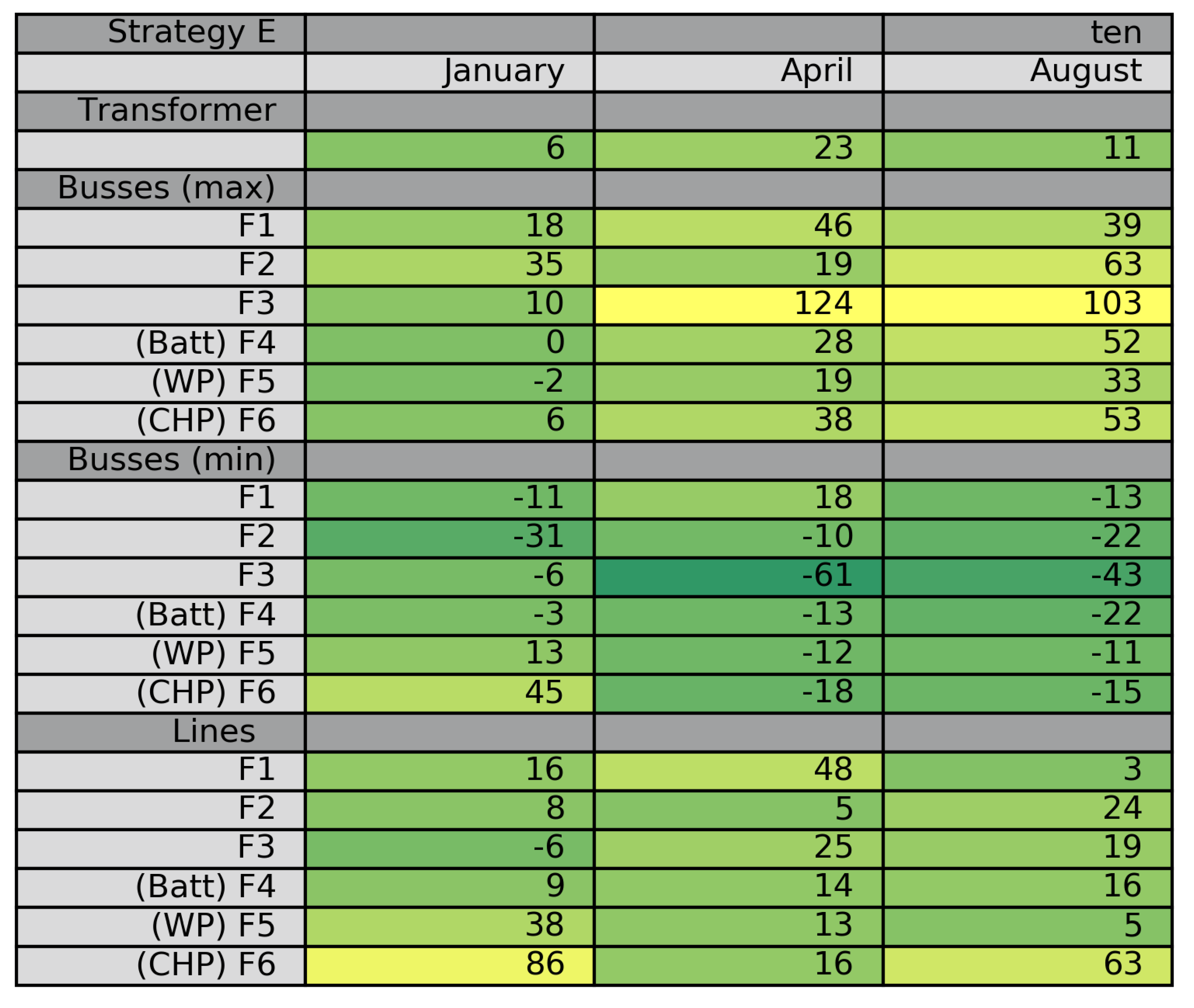
Strategy E diverges from the other strategies in terms of both the Basic-Grid and the Test-Grid configurations. The objective here is to analyze the influence of MES placement within the distribution grid. Consequently, the Basic-Grid mirrors the Test-Grid of Strategy A, featuring feeder-specific MES placement. This setup is then juxtaposed with another Test-Grid where MESs are randomly positioned across all six feeders. In both scenarios, MESs are distributed across all six feeders, allowing them to exert an impact on the distribution grid.

This leads to the following assumptions for the different strategies.

• Strategy A: “Feed-In incentives”

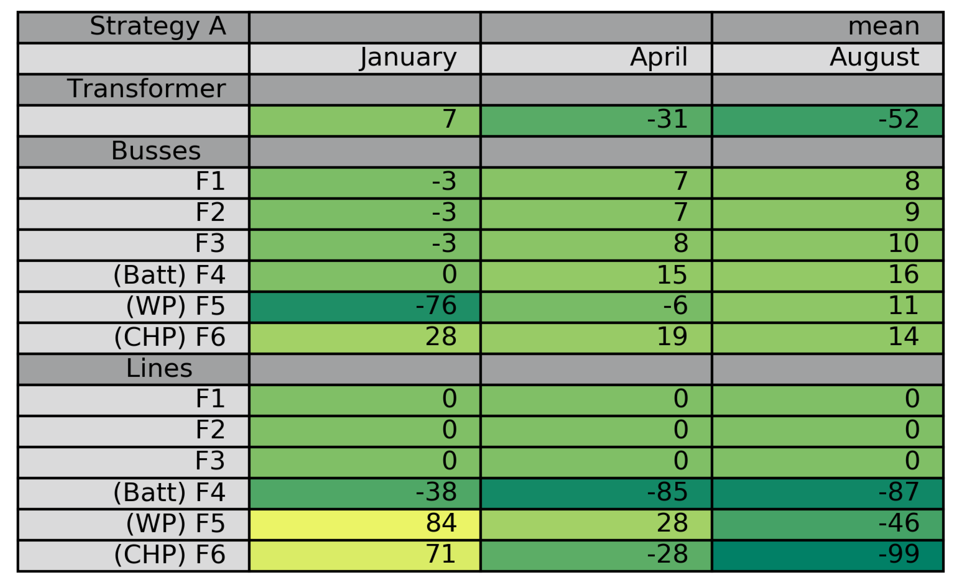
The Basic-Grid is configured as outlined earlier. Random electrical loads are generated for feeder 1, feeder 2, and feeder 3 using an artificial load profile generator based on German household statistics. Meanwhile, the electrical load profiles for feeder 4, feeder 5, and feeder six are assumed to be the same as those used for MES control optimization in Step 2. In Strategy A’s Test-Grid, the focus is on representing the prevailing systems currently in operation, reflecting the feed-in tariffs and incentives for PV and CHP systems in Germany. Control optimization is geared toward minimizing the MES’s operational costs. A perfect forecast is employed as the forecast method, ensuring no discrepancies between forecast PV production and energy consumption and the actual values.

• Strategy B: “Without incentives”

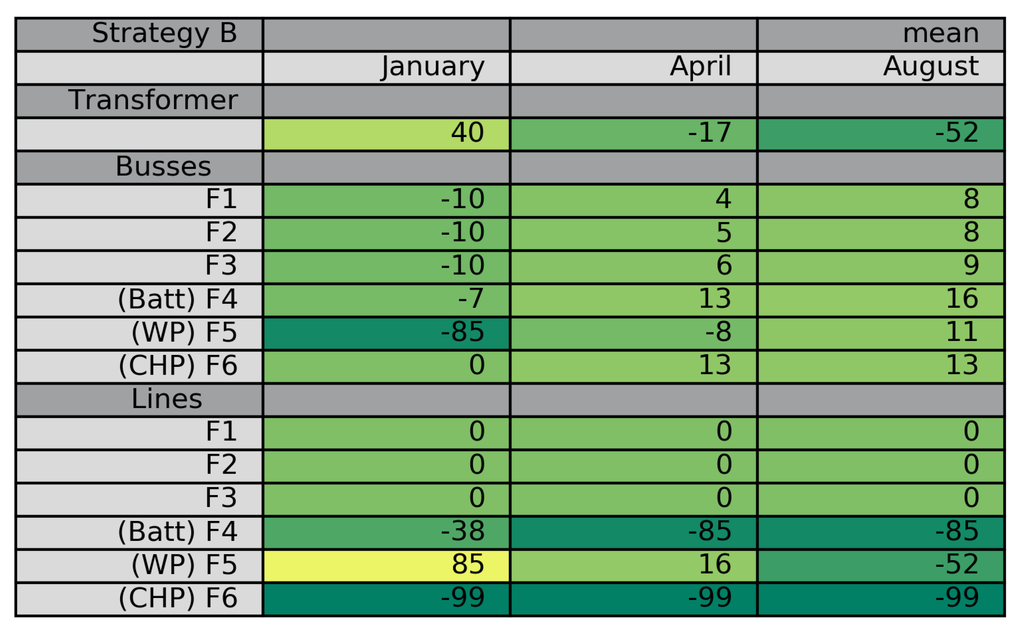
The Basic-Grid configuration remains consistent with Strategy A. In contrast, the Test-Grid is equipped with MESs operating without feed-in tariff contracts for energy produced by the PV and CHP systems. The control strategy is aimed at minimizing the operational costs of the multi-energy system, and the forecast method selected is perfect forecast, ensuring no discrepancies between forecasted PV production and energy consumption values and their actual counterparts.

• Strategy C: “CO₂ reduction”

The Basic-Grid configuration remains consistent with Strategy A. Conversely, the Test-Grid is equipped with MESs devoid of feed-in tariff contracts for energy produced by the PV and CHP systems. The control strategy is optimized for minimal CO₂ emission, and the forecast method selected is perfect forecast, ensuring no discrepancies between forecasted PV production and energy consumption values and their real counterparts.

• Strategy D “Market oriented”

The Basic-Grid configuration mirrors that of Strategy A. Conversely, the Test-Grid is outfitted with MESs lacking feed-in tariff contracts for energy produced by the PV and CHP systems. Instead, they receive a variable electricity price determined by a third party, such as the energy provider or a virtual power plant. The control strategy remains optimized for the operational costs of the multi-energy system, with a perfect forecast method chosen to ensure no disparities between forecasted PV production and energy consumption values and their actual counterparts.

• Strategy E “Random MES placement”

The Basic-Grid configuration is identical to the Test-Grid of Strategy A. However, in the Test-Grid, the placements of the MESs are randomized. All 23 consumers, including the MES, can be located at any bus within the grid.

2.4. Impact Analysis

To quantify the impact of different MESs on a distribution grid, I employed three distinct analysis methods. In grid expansion planning, it is crucial to consider the maximum and minimum values of voltage and asset loading to ensure grid stability under extreme conditions. This leads to the min/max value analysis (focusing solely on minimum and maximum values) and the extreme value analysis (examining 10% of the minimum and maximum values). In grid operation and asset management, understanding the average grid load and the overall utilization of grid assets is vital, especially when studying new grid control strategies or assessing the aging effects of cables and transformers. Hence, I conducted an analysis of average values through bulk value analysis. These analyses were performed separately for all six feeders in the grid, allowing for the examination of each MES type’s impact with different control strategies. Additionally, Strategy E evaluates the effect of randomly placed MESs on each feeder. (Refer to Figure 6 for more details).

2.4.1. Min/Max Value Analysis

To analyze the impact of the MES on the distribution grid, I compared a Basic-Grid configuration with a Test-Grid configuration. In the min/max value analysis, I focused solely on the maximum and minimum values. To assess the impact on transformers, I subtracted the maximum loading value for the chosen time period in the Test-Grid from the maximum loading of the Basic-Grid. Similarly, I compared the maximum line loading values and the maximum and minimum voltage values between the two configurations:

$$\begin{array}{ccc}\hfill \Delta T_{\max }& =& T_{\max }^{\mathrm{basic}}-T_{\max }^{\mathrm{test}}\hfill \end{array}$$

(7)

$$\begin{array}{ccc}\hfill \Delta L{X}_{\max }& =& L{X}_{\max }^{\mathrm{basic}}-L{X}_{\max }^{\mathrm{test}}\hfill \end{array}$$

(8)

$$\begin{array}{ccc}\hfill \Delta V{X}_{\max }& =& V{X}_{\max }^{\mathrm{basic}}-V{X}_{\max }^{\mathrm{test}}\hfill \end{array}$$

(9)

$$\begin{array}{ccc}\hfill \Delta V{X}_{\min }& =& V{X}_{\min }^{\mathrm{basic}}-V{X}_{\min }^{\mathrm{test}}\hfill \end{array}$$

(10)

with $X\in \{1,2,3,4,5,6\}$ is the number of the feeder; $T{X}_{\max }$ is the maximum of all transformer-loading values of the 9-day profile of each feeder for each time period (January, April, August), respectively; $L{X}_{\max }$ is the maximum of all line-loading values of the 9-day profile of each feeder for each time period (January, April, August), respectively; $V{X}_{\max }$ is the maximum of all bus voltage values of the 9-day profile of each feeder for each time period (January, April, August), respectively; and $V{X}_{\min }$ is the minimum of all bus voltage values of the 9-day profile of each feeder for each time period (January, April, August), respectively. See also Figure 6.

2.4.2. Extreme Values Analysis

In the second analysis, I considered that for grid planning and operation, it is not only the maximum and minimum values that are important, but also a certain range for the extreme values. To facilitate the comparison between the Test-Grid and the Basic-Grid, I computed the mean of the highest (exH) and lowest (exL) 10% values of the sorted time profile for each feeder X and each asset group (transformer, lines, buses):

$$\begin{array}{c}\hfill \Delta T_{\mathrm{exH}}=\sum _{\mathrm{i}=\mathrm{i}90}^{\mathrm{i}100}{T}_i^{\mathrm{basic}}/(N_T·0.1)-\sum _{\mathrm{i}=\mathrm{i}90}^{\mathrm{i}100}{T}_i^{\mathrm{test}}/(N_T·0.1)\end{array}$$

(11)

$$\begin{array}{c}\hfill \Delta L{X}_{\mathrm{exH}}=\sum _{\mathrm{i}=\mathrm{i}90}^{\mathrm{i}100}L{X}_i^{\mathrm{basic}}/(N_L·0.1)-\sum _{\mathrm{i}=\mathrm{i}90}^{\mathrm{i}100}L{X}_i^{\mathrm{test}}/(N_L·0.1)\end{array}$$

(12)

$$\begin{array}{c}\hfill \Delta V{X}_{\mathrm{exH}}=\sum _{\mathrm{i}=\mathrm{i}90}^{\mathrm{i}100}V{X}_i^{\mathrm{basic}}/(N_V·0.1)-\sum _{\mathrm{i}=\mathrm{i}90}^{\mathrm{i}100}V{X}_i^{\mathrm{test}}/(N_L·0.1)\end{array}$$

(13)

$$\begin{array}{c}\hfill \Delta V{X}_{\mathrm{exL}}=\sum _{\mathrm{i}=\mathrm{i}0}^{\mathrm{i}10}V{X}_i^{\mathrm{basic}}/(N_V·0.1)-\sum _{\mathrm{i}=\mathrm{i}0}^{\mathrm{i}10}V{X}_i^{\mathrm{test}}/(N_V·0.1)\end{array}$$

(14)

where $T{X}_i$ is the transformer loading, $L{X}_i$ is the line loading and $V{X}_i$ is the voltage at bin $i=iN$, and $iN$ is the bin number at the value that is at $N\%$ of the sorted sample (e.g., $i0=0,i100=\mathrm{10,376}$ (total number of values), $i10=1037$) for the Basic-Grid and Test-Grid, respectively. $N_Y·0.1$ is the number of the 10% values depending on the total numbers in the sample $\left(N_Y\right)$. The different values for each asset and feeder are equal to the number of lines and buses or transformers times the number of time steps in the studied time period.

2.4.3. Bulk Value Analysis

This third analysis method was selected to examine the overall average impact on the grid. In this approach, I compute the mean values of the second plus the third quartile (bulk) of the sorted time profiles for each feeder X and each time period.

$$\begin{array}{c}\hfill \Delta T_{\mathrm{bulk}}=\sum _{\mathrm{i}=\mathrm{i}25}^{\mathrm{i}75}{T}_i^{\mathrm{basic}}/(N_T·0.5)-\sum _{\mathrm{i}=\mathrm{i}25}^{\mathrm{i}75}{T}_i^{\mathrm{test}}/(N_T·0.5)\end{array}$$

(15)

$$\begin{array}{c}\hfill \Delta L{X}_{\mathrm{bulk}}=\sum _{\mathrm{i}=\mathrm{i}25}^{\mathrm{i}75}L{X}_i^{\mathrm{basic}}/(N_L·0.5)-\sum _{\mathrm{i}=\mathrm{i}25}^{\mathrm{i}75}L{X}_i^{\mathrm{test}}/(N_L·0.5)\end{array}$$

(16)

$$\begin{array}{c}\hfill \Delta V{X}_{\mathrm{bulk}}=\sum _{\mathrm{i}=\mathrm{i}25}^{\mathrm{i}75}V{X}_i^{\mathrm{basic}}/(N_V·0.5)-\sum _{\mathrm{i}=\mathrm{i}25}^{\mathrm{i}75}V{X}_i^{\mathrm{test}}/(N_V·0.5).\end{array}$$

(17)

In the provided formulas, $T{X}_i$ represents transformer loading, $L{X}_i$ denotes line loading, and $V{X}_i$ stands for the voltage at bin $i=iN$. Here, $iN$ refers to the bin number corresponding to the value at $N\%$ of the sorted sample for both the Basic-Grid and Test-Grid. The term $N_Y·0.5$ denotes half of the number of values at the 50% mark, dependent on the total number of values in the sample ($N_Y$). The varying number of values for each asset and each feeder is equivalent to the number of lines and buses or transformers multiplied by the number of time steps in the analyzed period.

3. Results

In the preceding Methods and Materials section, I outlined my toolchain and reported the outcomes of Step 1: Load Profile Generator and Step 2: MES Simulation. Now, in this Results section, our focus shifts toward addressing the core scientific inquiry: What is the impact of various MES types with distinct control strategies on low-voltage distribution grids?

To begin, I will present the findings derived from the time-series-based load flow simulation conducted using pandapower for the introduced low-voltage grid. While the comprehensive presentation of all results, including those illustrated in Figure A4, Figure A5, Figure A6, Figure A7, Figure A8, is beyond the scope of this paper, I will emphasize this study’s principal discoveries.

Following this, in the subsequent section, I will leverage the outcomes of the load flow simulation as input for the newly developed statistical impact analysis from Step 4. This analysis will explore the implications of MES integration on the power grid by examining the impact results of the three analysis methods outlined in Equations (8)–(17) for each control, Strategies A to E. By doing so, I aim to identify the key features that necessitate consideration when integrating MESs into the power grid.

Before delving into these findings, I will provide examples of resulting profiles from the time-series-based grid calculation.

3.1. Results from Time-Series-Based Load Flow Simulation

The time-series-based load flow calculation yields voltage values for each bus, loading for each line, and loading for the transformer. This calculation is conducted separately for all lines, buses, and transformers in all six feeders, with 144 time steps per day for three 9-day periods. Consequently, over 100,000 values per feeder are evaluated to gauge the impact of MESs on the distribution grid. Additionally, results are available for all five previously defined MES control strategies. To understand the results of the time-series based power-grid simulation, the results for Strategy A are shown exemplarily in Figure 7, Figure 8 and Figure 9 for the lines and buses of feeders 4, 5, and 6 and the transformer here for the 8th day of April. The results for the 9-day period are depicted in the Appendix C. The box plots show the result for each time step for all bussed or lines and transformers in the chosen feeder and grid. The error bars of the results show the differences between the buses or lines in each feeder. On the left side, the numbers for the Basic-Grid calculation are shown for Strategy A for each feeder, while on the right side, the results for the Test-Grid, including the MESs, are presented. The first rows in Figure 7 and Figure 8 show the results for feeder 4, including the PV-battery systems; the second row is for feeder 5, including the PV-HP systems; and the third row is feeder 6, including the PV-CHP systems.

In Figure 7, the left-hand column displays the calculated line loadings for the basic grid. These time-series depict the impact of typical residential load profiles on the distribution grid, with occasional extreme values observed around noon. Conversely, in the right-hand column, the line loading profiles calculated for the Test-Grid exhibit distinctive shapes compared to the grid impact of typical load profiles. Depending on the MES, the grid time-series exhibits significant variation. Analyzing the results in feeder 4, representing the impact of PV-battery systems, reveals disruptions in the PV peak from 9 to 14 h due to battery charging. Moreover, the battery’s discharge balances the household load during the first 5 h of the day, resulting in minimal interactions with the grid. For feeder 5, featuring installed PV-HP systems, the line loading profiles demonstrate variations. Higher line loading is observed in the morning and evening due to the additional electrical load from the HP. PV energy is utilized throughout the day to fulfill the HP and household load requirements, leading to a dip in line loading from 11 to 15 h. In feeder 6, where PV-CHP systems are installed, a distinct trend in line loading emerges. Here, both PV energy and portions of CHP energy are fed into the grid, resulting in significantly high peak line loading from 9 to 18 h.

In Figure 8, the left-hand column panels display voltage time-series dominated by typical household load profiles, exhibiting values below 1 PU. Conversely, the panels in the right column illustrate results for the Test-Grid, showcasing distinct outcomes depending on the MES connected to the feeder. For feeder 4 with PV-battery systems, a peak resulting from PV electricity fed into the grid is evident. The primary impact stems from the additional PV system generating electricity, with its output managed by the battery. In feeder 5, featuring PV-HP systems, the difference from the load is relatively flat during noon, despite the PV energy, which is primarily consumed by the HP and not fed into the grid. The introduction of a new electrical HP load leads to additional peaks below 1 PU. The primary impact of the PV-HP MES is attributed to the additional electrical load. In feeder 6, with PV-CHP systems, additional energy is injected into the grid. Both PV and CHP systems generate electricity that cannot be fully consumed by the household, resulting in high voltage values around noon. Due to the self-produced energy, values below 1 PU are not visible. The grid’s impact arises from injected energy rather than consumed energy.

In Figure 9, the loadings for the transformer for Strategy A in the transition period of April are depicted. As there is only one transformer present, the box plot here encompasses the values over time for the 144 time steps of the chosen day. A comparison reveals that the overall loading values fall almost within the same range for both grids. The mean value, though, is lower for the grid with multi-energy systems controlled by Strategy A. This implies that the impact on the transformer is less pronounced with MESs than with household loads only. The integration of new decentralized generation and consumption units in feeders 4, 5, and 6 results in a reduced energy flow through the transformer. Consequently, the region exhibits higher self-sufficiency and requires less energy from outside sources.

The values presented in this section for Strategy A, covering the complete 9-day periods in summer, winter, and the transition time period, along with the corresponding results for the other strategies, are then utilized in Step 4 to obtain the results for the statistical analysis of the impact of MESs on a distribution grid.

3.2. Statistical Analysis

Since the analysis yields numerous resulting values, two methods of presenting the results are introduced. The first method utilizes bar graphs, as displayed in Figure 10, Figure 11 and Figure 12 for the summer, winter, and transition periods, respectively. The second method involves a table with color-coded values, as depicted in Appendix D. In this section, I will discuss the impact findings. For details on the second method, please refer to the explanation in the Appendix D.

The results of the impact analysis are all shown in one overview in Figure 10, Figure 11 and Figure 12. The upper panel shows the values of the min/max analysis, the middle panel shows the extreme value analysis results, and the lower panel depicts the bulk value analysis results. The different colors stand for the five different control strategies, as shown in the figure caption. The labels on the left side belong to the voltage values, while the labels on the right hand side of the panels belong to the loadings. The numbers were calculated as described in the Materials and Methods section in Equations (8)–(17). To understand Figure, I would like to remind readers of the idea of comparing the values from the time-series grid simulation from the Basic-Grid and the Test-Grid. Therefore, the results show the difference between those two grids. The larger the bars, the larger the difference and, therefore, the larger the impact of the MESs on the grid. The positive values stand for a higher impact, which can be a higher current in the cables and the transformer, a higher voltage in the buses in the feed-in-dominated case, and lower voltage in the buses in the load-dominated case when compared with the Basic-Grid. This means that I can not only analyze in great detail the size of the impact but also derive the impact for each MES, each control strategy, and even the impact of the placement of the MES within the grid when looking at the bars of feeders 4, 5 and 6. Feeder 1, feeder 2, and feeder 3 are shown as a kind of benchmark. In these feeders, nothing is changed in four of the five strategies, and no MES is installed. Only in Strategy E (red color), where the MESs are placed randomly, are the results for these feeders also changing. So, in the following, I will discuss the results mainly for feeder 4 (PV-battery systems), feeder 5 (PV-HP systems), feeder 6 (PV-CHP systems), and the transformer.

The results of the impact analysis are presented comprehensively in Figure 10, Figure 11 and Figure 12. Each figure comprises three panels: the upper panel displays the values of the min/max analysis, the middle panel shows the extreme value analysis results, and the lower panel depicts the bulk value analysis results. The colors correspond to the five different control strategies, as indicated in the figure caption. Voltage values are labeled on the left side of the panels, while loadings are labeled on the right-hand side. These numbers were calculated according to the method described in the Materials and Methods section (Equations (8)–(17)). To interpret the figures, it is important to recall the basic idea of the method, which is the comparison between the values from the time-series grid simulation for the Basic-Grid and the Test-Grid. Therefore, the results represent the difference between these two grids. Larger bars indicate a greater difference and, thus, a higher impact on the grid by the MES systems. Positive values signify a higher impact, which could manifest as increased current in the cables and the transformer, higher voltage in the buses in the feed-in-dominated case, and lower voltage in the buses in the load-dominated case compared to the Basic-Grid. This allows for a detailed analysis of the impact of each MES, each control strategy, and even the placement of the MESs within the grid, as observed through the bars of feeders 4, 5, and 6. Feeders 1, 2, and 3 serve as benchmarks, with no changes in four of the five strategies, indicating the absence of installed MESs. Only in Strategy E (red color), where the MESs are randomly placed, do the results for these feeders change. Therefore, the discussion primarily focuses on feeder 4 (PV-battery systems), feeder 5 (PV-HP systems), feeder 6 (PV-CHP systems), and the transformer.

• Impact on the transformer $\Delta T$

For the time period in August, the analysis reveals significant impacts on the transformer. The newly installed PV systems result in much higher extreme values, with $\Delta V{X}_{\max }\approx 0.12$–$0.15\%$ and $\Delta V{X}_{\mathrm{exH}}\approx 0.8$–$1.0\%$. However, Strategy E shows varying percentages depending on the placement of the MESs. The transformer exhibits approximately $\Delta T_{\max }\approx 10\%$ and $\Delta T_{\max }\approx 20\%$ higher loadings for almost all control strategies, including MESs, for the maximum value and the 10% highest values of the time period, respectively. Conversely, the overall bulk values show a 50% reduction for all control strategies. The impact on the transformer in August is dominated by PV systems in peak values, while the bulk values are reduced due to higher self-sufficiency in the grid region.

• Impact on the buses $\Delta V$

The reduced load due to the higher self-consumption of the MES results in higher voltage values in the Test-Grid compared with the Basic-Grid. This leads to negative percentages $\Delta V{X}_{\min }\approx 0.05\%$ and $\Delta V{X}_{\mathrm{exL}}\approx 0.3\%$ for almost all MES control strategies. However, this effect is smaller for Strategy E, resulting in a higher impact in feeder 1 to feeder 3. The impact of the MES in August on the voltage peak values is dominated by the PV systems.

• Impact on the lines and cables $\Delta I$

The line loadings exhibit similar trends across all strategies but are smaller for Strategy E. The extreme values are higher by $\Delta L{X}_{\max }\approx 30$–$55\%$ and $\Delta L{X}_{\mathrm{exH}}\approx 40$–$65\%$, indicating increased energy flow due to the PV systems. However, the bulk values show smaller line loading values of 80% for the PV-battery system, 50% for PV-HP systems, and almost 100% for the PV-CHP system for Strategies A, B, and D. Strategy C, minimizing CO₂ output, only achieves 80%, suggesting reduced CHP usage. In summary, PV and CHP energy production dominate extreme values, while average line and transformer loadings decrease due to the local energy production and consumption.

3.2.1. August—The Summer Period

• Impact on the transformer $\Delta$T

For the time period in August, the analysis reveals that the newly installed PV systems lead to much higher extreme values of about $\Delta V{X}_{\max }\approx 0.12$–$0.15\%$ and for $\Delta V{X}_{\mathrm{exH}}\approx 0.8$–$1.0\%$. Only Strategy E shows lower percentages for feeders 4, 5, and 6 and higher percentages for feeders 1, 2, and 3, depending on the new placement of the MESs. The transformer exhibits approximately $\Delta T_{\max }\approx 10\%$ and $\Delta T_{\max }\approx 20\%$ higher loadings for almost all control strategies, including the MESs, for the maximum value and the 10% highest values of the time period, respectively. However, the overall bulk values show an impact with 50% lower values for all control strategies. The impact on the transformer is dominated in August by the PV systems in the peak values, but the bulk values are reduced due to a higher self-sufficiency in the grid region.

• Impact on the buses $\Delta$V

The reduced load due to the higher self-consumption of the MESs results in higher voltage values of the Test-Grid compared with the Basic-Grid, leading to negative percentages $\Delta V{X}_{\min }\approx 0.05\%$ and $\Delta V{X}_{\mathrm{exL}}\approx 0.3\%$ for almost all MES control strategies. This effect is smaller for Strategy E, leading to a higher effect in feeder 1 to feeder 3. The impact of the MES in August on the voltage peak values is dominated by the PV systems.

• Impact on the lines and cables $\Delta$I

The line loadings exhibit the same trend for all strategies, but less for Strategy E. The extreme values are higher by $\Delta L{X}_{\max }\approx 30$–$55\%$ and $\Delta L{X}_{\mathrm{exH}}\approx 40$–$65\%$. This is because more energy, due to the PV systems, is running through the lines. However, the bulk values show smaller line loading values of 80% for the PV-battery system, 50% for PV-HP systems, and almost 100% for the PV-CHP system for Strategies A, B, and D. Strategy C, which minimizes CO₂ output, only has values of 80%. The bulk values are changed due to more electricity being produced by the CHP. The 80% value for the CO₂ strategy is indicating that the CHP is not used as often as in the other strategies and has therefore a reduced impact on the grid.

In summary, it is interesting to note that the PV and CHP energy productions dominate the grid impact of extreme values, but the average line and transformer loadings are reduced due to the local production and consumption of energy.

3.2.2. August—Summer Period

• Impact on the transformer $\Delta$T

For August, the impact analysis reveals significant effects on the transformer. The newly installed PV systems result in much higher extreme values, with $\Delta V{X}_{\max }\approx 0.12$–$0.15\%$ and $\Delta V{X}_{\mathrm{exH}}\approx 0.8$–$1.0\%$. However, Strategy E shows varying percentages depending on the placement of the MESs. The transformer exhibits approximately $\Delta T_{\max }\approx 10\%$ and $\Delta T_{\max }\approx 20\%$ higher loadings for almost all control strategies, including MESs, for the maximum value and the 10% highest values of the time period, respectively. Conversely, the overall bulk values show a 50% reduction for all control strategies. The impact on the transformer in August is dominated by PV systems in peak values, while the bulk values are reduced due to higher self-sufficiency in the grid region.

• Impact on the buses $\Delta$V

The reduced load due to the higher self-consumption of the MES results in higher voltage values of the Test-Grid compared with the Basic-Grid, leading to negative percentages $\Delta V{X}_{\min }\approx 0.05\%$ and $\Delta V{X}_{\mathrm{exL}}\approx 0.3\%$ for almost all MES control strategies. This effect is smaller for Strategy E, leading to a higher effect in feeder 1 to feeder 3. The impact of the MES in August on the voltage peak values is dominated by the PV systems.

• Impact on the lines and cables $\Delta$I

The line loadings exhibit similar trends across all strategies, but they are smaller for Strategy E. The extreme values are higher by $\Delta L{X}_{\max }\approx 30$–$55\%$ and $\Delta L{X}_{\mathrm{exH}}\approx 40$–$65\%$, indicating increased energy flow due to the PV systems. However, the bulk values show smaller line loading values of 80% for the PV-battery system, 50% for the PV-HP system, and almost 100% for the PV-CHP system for Strategies A, B, and D. Strategy C, which minimizes CO₂ output, only achieves 80%. The bulk values are changed due to more electricity being produced by the CHP. The 80% value for the CO₂ strategy indicates that the CHP is not used as often as in the other strategies and has, therefore, a reduced impact on the grid.

In summary, PV and CHP energy productions dominate the grid impact of extreme values, but the average line and transformer loadings are reduced due to the local energy production and consumption.

3.2.3. January—Winter Period

The impact of the MES in winter is generally smaller and more concentrated on systems with heating in feeders 5 and 6.

• Impact on the transformer $\Delta$T

The impact on transformer loading is relatively small compared to the Basic-Grid, with bar sizes indicating minor differences.

• Impact on the buses $\Delta$V

For Strategy A in feeder 6, there is a slight increase in voltage values, with $\Delta V{X}_{\min }\approx 1.2\%$ and $\Delta V{X}_{\mathrm{exL}}\approx 0.6\%$, attributed to the PV and CHP energy fed into the grid. In feeder 5, with PV-HP systems, significant impacts are observed due to higher electrical loads for heating, resulting in a $\Delta V{5}_{\min }$ of up to 4% and $\Delta V{5}_{\mathrm{exL}}$ of up to 1.8%. Strategy E distributes the effect across all six feeders due to the MES placement.

• Impact on the lines and cables $\Delta$I

Feeder 5, with PV-HP systems, shows substantial impacts, with $\Delta L{5}_{\max }\approx 30$–$55\%$ and $\Delta L{5}_{\mathrm{exH}}$ values of up to 80%. Feeder 6, with PV-CHP systems, exhibits similar trends in extreme line loading values, but different control strategies produce varied impacts on the bulk values. Strategies A and E lead to higher values of up to 75%, while others show reductions of up to −90%. Feeder 4, with PV-battery systems, and feeder 5, with PV-HP systems, experience unusual differences of 150% to 400$ for minimum voltage values, suggesting infrequent but extreme occurrences possibly due to electrical heating effects.

3.2.4. April—Transition Period

Indeed, the observed impact trends from both the summer and winter periods appear to be present in the transition period. This is understandable considering the coexistence of a decentralized energy production and heating demand, leading to an increased usage of heat pumps (HPs) and combined heat and power (CHP) systems. While the impact may not be as extreme as in the winter and summer periods, it is more diverse across feeders, lines, and buses.

In summary, three main features of MESs have a significant impact on distribution power grids. Firstly, the presence and size of PV systems notably affect the grid’s maximum and 10% extreme values. Secondly, MESs with CHP and HP units, adding additional electricity into the grid, influence the grid’s overall performance, as represented by the bulk values. Thirdly, the placement of MESs with heating systems plays a role, indicating that the maximum needed power has a large impact on the grid, particularly when systems are clustered in one feeder. Interestingly, the impact of an MES does not vary significantly across different control strategies.

4. Summary and Discussion

The method presented in this study offers a comprehensive approach to assessing the impact of MESs on distribution grids without the need for fixed voltage and current limits. In analyzing characteristic features, including extreme and bulk values, this method enables the derivation of measures to plan a stable grid, providing valuable insights for management strategies.

The evaluation of five different strategies revealed that, aside from variations in placement observed in Strategy E, the overall impact on the grid remains similar across strategies. Notably, while extreme values are affected by an increased electrical energy production (e.g., from PV and CHP) and consumption (e.g., from HP), the overall grid workload often decreases due to higher self-consumption rates in MESs.

The extreme values are shifting as anticipated with the increased electrical energy production (PV, CHP) and consumption (HP). However, it is noteworthy that the overall grid workload is frequently diminished due to the heightened self-consumption rates in MESs.

The disparity between the 10% extreme value analysis and the min/max value analysis serves as an indicator of the frequency of occurrence of minimum values. When the 10% extreme values significantly diverge from the minimum or maximum values, this suggests infrequent occurrences during the specified time period. Conversely, if they closely align, it implies that such extreme impacts are more frequent. These findings are instrumental in devising tailored solutions to address grid challenges, as they provide insights into the frequency and severity of grid disturbances.

The distinction between cost or CO₂ optimization holds little relevance for the impact on a low-voltage grid, with the exception of PV-CHP systems.

The outcomes from Strategy E underscore the necessity to analyze the impact of an optimized MES individually in each feeder. Understanding whether the clustering of similar MESs occurs is crucial, as it alters the grid’s impact.

The analyzed MESs exhibit varied behaviors based on their energy production, storage, and consumption components. While they generally behave similarly during the summer period, owing to the presence of installed PV systems, their distinctions become apparent in the winter season. Specifically, the simultaneous generation of thermal energy by both HP and CHP systems, with HPs consuming electrical energy and CHP producing it, results in contrasting impacts on the distribution grid’s voltage extreme values. Furthermore, local combinations of HP and CHP systems can mitigate the grid’s impact during the winter.

This study also highlights the importance of assessing MES impacts across different seasons. While PV systems dominate in the summer and heating systems in the winter, the transition period presents a combination of effects, making impact prediction challenging, especially with multiple energy production and consumption units present.

Looking ahead, challenges remain in conducting yearly simulations efficiently due to computational demands. Enhancing the performance of models and establishing automated connections between them are crucial steps for assessing the impact of MESs on real distribution grids over extended periods, thereby informing future grid management strategies.

4.1. Sensitivity Analysis

After discussing certain aspects and results, I will conclude this chapter by analyzing the potential impact of three additional control strategy ideas and how they could alter the outcomes. These include evaluating the impact of MESs when a PV system is already installed, analyzing the effect of forecast deviations, and assessing the impact when the idea of peak shaving is applied.

4.1.1. Strategy A: Retrofit Solution—PV Is Already Installed

Up to now, I have assumed that the households in the Basic-Grid have not been equipped with PV systems. The assumption would be that the households in feeder 4, feeder 5, and feeder 6—each feeder may be owned by the same person—are going to install complete multi-energy systems, including PV systems. In reality, PV systems are already common in residential areas. I would like to know the impact on the grid of MESs when PV systems are already present. For the maximum impact, I assume now that all houses are equipped with PV systems for the Basic-Grid. The households of feeder 4, feeder 5, and feeder 6 are treated as in Strategy A. They will retrofit their PV systems with HP, CHP, and battery systems as described above. As a result, the impact is different. The Basic-Grid profiles already show a PV peak in voltage and line loading numbers. In looking at the results with MESs, the impact is much smaller. But in looking, e.g., at feeder 5 (PV-HP system), the voltage profile in Figure 13 shows, in April, a much smaller PV peak, and in the morning and in the evening, very low voltage values are observed due to the electricity needed for the HP. Also, the line loading shown in Figure 14 shows much higher values in the morning and in the evening, but due to the high self-consumption of the PV energy, very small values during noon. Here, the impact of MESs can be even larger depending on the MES.

Under the assumption that households in feeders 4, 5, and 6 are already equipped with PV systems in the Basic-Grid scenario, the addition of MESs introduces a different impact on the grid. In this scenario, the Basic-Grid profiles already exhibit a PV peak in voltage and line loading values. However, with the introduction of MESs, the impact becomes less pronounced. For instance, in considering feeder 5 with a PV-HP system, the voltage profile during April shows a reduced PV peak, with lower voltage values in the morning and evening due to the electricity required for the HP. Similarly, the line loading exhibits higher values in the morning and evening, but with smaller values during noon due to the high self-consumption of PV energy. Consequently, the impact of MESs in this scenario may vary depending on the specific MES implemented. In summary, while the presence of existing PV systems in the Basic-Grid scenario mitigates the overall impact of MESs, the specific characteristics of the MESs, such as the introduction of HP or CHP systems, can still significantly influence the grid performance, particularly during peak demand periods.

4.1.2. Strategy A with Persistent Forecast for the PV-CHP Systems

In the analysis, I assumed a perfect forecast for all control strategies. However, in reality, forecasts may deviate from actual values, thereby affecting grid profiles and their impact. To model this deviation, a secondary control is introduced to the simulation environment, as described in [32]. Here, I compare the results of Strategy A with a perfect forecast against those with imperfect forecasts. In Figure 15, the differences in values for the lines and buses are presented. Generally, forecast deviations lead to higher line loading values and higher voltages (>1PU), as well as lower voltages (<1PU). The effect is typically less than 10%.

4.1.3. Grid-Friendly Peak Shaving

In [29], another strategy was explored, involving the implementation of grid-friendly behavior in MESs through forced peak shaving. The concept entails allowing only a certain percentage (e.g., 50%) of the installed PV capacity to be injected into the grid, thereby reducing the impact of PV systems, especially during the summer. An optimized MES could incorporate this limit, diverting excess energy for self-consumption. It has been demonstrated that this approach is feasible, albeit requiring a larger battery for added flexibility. This new control strategy has the potential to decrease the impact of extreme values by a few percentage points, particularly during the summer period. The peak-shaving mechanism can be integrated into all control strategies discussed in this study.

The sensitivity analysis explores the impact of different scenarios on the grid performance, including cases where households are already equipped with PV systems and variations in the forecast accuracy for PV-CHP systems. The results indicate that pre-existing PV systems in households mitigate the overall impact of MESs, while deviations in the forecast accuracy can lead to slight changes in grid profiles, underscoring the importance of accurate forecasting for effective grid management.

5. Conclusions

The results of this study shed light on the intricate dynamics between MESs and distribution power grids, providing insights that resonate with previous research and working hypotheses. Focusing first on the results from the MES type and placement, firstly, the observed impacts of MESs on the grid performance align with expectations derived from prior studies. The presence and size of photovoltaic (PV) systems are identified as significant factors influencing the grid’s extreme values, corroborating findings from various studies highlighting the importance of distributed solar generation. Similarly, the introduction of MESs with combined heat and power (CHP) and heat pump (HP) units is shown to affect the grid’s overall performance, particularly in terms of bulk values, which is consistent with the anticipated implications of introducing additional electricity into the grid. Furthermore, the examination of MES placement within the grid reveals nuanced insights into the varying impacts across different feeder systems. The clustering of MESs with heating systems in specific feeders is found to amplify the grid’s vulnerability to high-demand scenarios, underlining the importance of considering local energy dynamics when planning MES deployment. The findings from this study also have significant implications for grid planning, operation, and management strategies. Firstly, the methodology highlights the importance of considering regional variations in grid infrastructure and energy consumption patterns, which can greatly influence the performances of multi-energy systems (MES). This understanding is crucial for developing tailored grid planning strategies that accommodate the specific needs and characteristics of different regions. Secondly, the results demonstrate that the integration of MESs can lead to higher self-consumption rates, which in turn reduces the overall workload on the grid. This insight can inform grid operation strategies aimed at optimizing the balance between energy production and consumption, thereby enhancing grid stability and efficiency. Thirdly, this study underscores the necessity of accounting for the clustering of similar MESs within specific feeders. This factor can significantly alter the grid’s impact, making it essential for grid management strategies to include detailed analyses of the MES distribution and clustering effects. Interestingly, the analysis indicates that the impact of MESs remains relatively consistent across different control strategies. Despite variations in grid profiles resulting from different control strategies, the fundamental impacts on buses, lines, and transformers show no significant differences. This finding challenges previous assumptions that varying control strategies would lead to distinct impacts on the grid performance, suggesting a need for more nuanced approaches to grid management. Moreover, the exploration of strategies such as forced peak shaving highlights potential avenues for mitigating the impact of MESs on grid extreme values, particularly during peak demand periods. The integration of such strategies into MES control frameworks offers promising opportunities for enhancing grid stability and resilience.

From a broader perspective, these findings underscore the complex interplay between distributed energy resources and grid infrastructure, emphasizing the importance of holistic approaches to energy system planning and management. Future research directions may focus on refining control strategies to optimize the grid integration of MESs, exploring novel technologies and methodologies for grid-friendly behavior and investigating the socio-economic implications of widespread MES deployment. This study serves as a proof-of-concept for the new methodology developed to assess the impact of MESs on distribution grids. The results indicate that this method is promising for understanding grid dynamics under various energy management strategies. However, further research is necessary to validate these findings against more extensive network data. In future research, I will apply the methodology to larger datasets, including the SimBench networks (www.simbench.de) [REF to SimBench] and real grid data obtained through collaboration with grid operators. This approach will allow me to rigorously validate the new grid impact method and ensure its reliability and accuracy. This methodology considers potential limitations and uncertainties, addressing data availability using both simulated demand profiles and accessible real-world data, such as weather, PV data, and MES parameters. I modeled each aspect as realistically as possible, from the energy demand to the network load flow calculations. Model assumptions were critically evaluated through time-series simulations across all seasons. Using a simple, generic low-voltage distribution grid model, I ensured that the impact of MESs is clear and not conflated with complex grid topology. While some assumptions may simplify complex real-world conditions, continuous refinement and validation against empirical data remain integral to future research efforts. Future research directions stemming from the proposed methodology include exploring the socio-economic implications of MES deployment and integrating emerging technologies. Socio-economic research could focus on analyzing the cost–benefit aspects of MESs for different stakeholder groups, assessing the impact on variable electricity prices, and evaluating potential economic incentives for adopting MESs. Additionally, the methodology could be expanded to incorporate emerging technologies such as advanced energy storage systems, electric vehicle wall boxes, hydrogen energy systems, smart meters, and energy trading platforms. These technologies can enhance grid management and improve the efficiency of MESs. Integrating these innovations will provide a more comprehensive understanding of how MESs can contribute to a sustainable and economically viable energy future. While this study provides valuable insights into the impact of MESs on grid planning, operation, and management, a wider sensitivity analysis exploring additional scenarios such as varying levels of photovoltaic penetration, battery capacities, and the impact of demand response programs will be conducted in future research to further enrich this study’s findings. Future research directions also include exploring the socio-economic implications of MES deployment, such as analyzing the cost–benefit aspects for different stakeholders, assessing the impact on electricity prices, and evaluating economic incentives for MES adoption. Additionally, the methodology can be expanded to integrate emerging technologies, such as advanced energy storage systems, electric vehicle wall boxes, hydrogen energy systems, smart meters, and energy trading platforms. These innovations will provide a more comprehensive understanding of how MESs can contribute to a sustainable and economically viable energy future. In incorporating these insights into grid planning, operation, and management strategies, the integration of MESs can be optimized to enhance grid performance and support the transition to a more sustainable energy system.

In conclusion, this study contributes valuable insights into the impacts of MESs on distribution power grids, offering a deeper understanding of the challenges and opportunities associated with the transition to decentralized energy systems. By elucidating the dynamics between MESs and the grid performance, this research informs policy-makers, energy planners, and stakeholders in shaping more resilient and sustainable energy futures.