Interpretability and Transparency of Machine Learning in File Fragment Analysis with Explainable Artificial Intelligence

Abstract

Machine learning models are increasingly being used across diverse fields, including file fragment classification. As these models become more prevalent, it is crucial to understand and interpret their decision-making processes to ensure accountability, transparency, and trust. This research investigates the interpretability of four machine learning models used for file fragment classification through the lens of Explainable Artificial Intelligence (XAI) techniques. Specifically, we employ two prominent XAI methods, Shapley Additive Explanations (SHAP) and Local Interpretable Model-Agnostic Explanations (LIME), to shed light on the black-box nature of four machine learning models used for file fragment classification. By conducting a detailed analysis of the SHAP and LIME explanations, we demonstrate the effectiveness of these techniques in improving the interpretability of the models’ decision-making processes. Our analysis reveals that these XAI techniques effectively identify key features influencing each model’s predictions. The results also showed features that were critical to predicting specific classes. The ability to interpret and validate the decisions made by machine learning models in file fragment classification can enhance trust in these models and inform improvements for better accuracy and reliability. Our research highlights the importance of XAI techniques in promoting transparency and accountability in the application of machine learning models across diverse domains.

1. Introduction

File fragment classification is a crucial technique useful in cybersecurity, digital forensics, and data recovery. In file fragment classification, file fragments are classified by their file type [1]. This task plays a critical role across a wide range of applications. Accurately classifying file fragments in forensic investigations is pivotal for reconstructing digital evidence and understanding cyber incidents. Law enforcement agencies and cybersecurity professionals can use this capability to solve digital crimes.

File fragment classification is also an integral component of malware detection systems. By scrutinizing the byte-level features of file fragments, these systems can identify patterns indicative of malicious code or behavior and correctly classify the files or fragments as malware [2]. Additionally, in data recovery, classifying file fragments assists in reconstructing damaged or corrupted files, which contributes to the restoration of valuable information. As the cybersecurity and digital forensics landscape continues to evolve, file fragment classification plays an increasingly important role in addressing multifaceted challenges.

In the past, diverse techniques have been employed for the implementation of file fragment classification. One prevalent approach involves statistical models, where the analysis of byte-level content is conducted using statistical metrics. These models leverage statistical measures such as entropy, frequency distribution, and n-gram analysis to discern patterns and characteristics within file fragments. These statistical models provide a foundational understanding of the inherent structure of files. Additionally, machine learning techniques can be utilized for file fragment classification. To achieve accurate file fragment classification, machine learning, and deep learning techniques have been employed. Machine learning has shown promising results in scenarios where the nuances of file fragments demand a more intricate understanding.

The field of machine learning (ML) and deep learning specifically has experienced significant advancements in various domains such as data analysis, image processing, computer vision, speech recognition, and natural language processing [3,4]. This continuous growth has led to the development of various ML models that can perform complex tasks with high accuracy and efficiency. ML models have subsequently been used for file fragment classification for these reasons. Furthermore, using machine learning for file fragment classification has seen significant success over the years [1]. It has become a popular approach due to its ability to handle large datasets and extract meaningful patterns from fragmented data. These models automatically learn and adapt to patterns in file fragments. Machine learning models for file fragment classification aim to accurately categorize fragments of files based on their content or patterns in the content.

However, as the role of AI and ML continues to expand and the results become more accurate and efficient, there is a growing need for transparency and interpretability in these models. The increasing complexity and black-box nature of these machine learning models pose a challenge to understanding their decision-making process. While traditional machine learning metrics like accuracy, confusion matrix, and classification report exist, they do not provide enough assurance about the model’s performance and reliability to users and stakeholders. This might be the case with a machine learning model that gives very high accuracy but fails to recognize some dataset classes because it uses irrelevant features. For instance, an image classification model used to classify two entities can utilize background pixels to recognize an object in an image rather than actual entity object pixels. This may affect the overall model prediction. Explainable Artificial Intelligence (XAI) has emerged to address these challenges.

Explainable Artificial Intelligence is a relatively new subfield in artificial intelligence which generally refers to techniques used to analyze the decision-making process of ML models [5]. It focuses on developing techniques and methodologies that enable humans to understand and interpret the decisions made by machine learning models. Explainable artificial intelligence aims to provide meaningful explanations for the outcomes produced by AI models, enhancing transparency and understanding of their reasoning [6]. Explainable AI makes artificial intelligence models more manageable and understandable. This helps users determine if an AI system is working as intended and quickly uncover any errors. It also helps build trust and confidence among an AI system’s users.

Furthermore, XAI techniques can also help identify and address biases or unfairness in machine learning models. XAI allows for identifying and mitigating bias in the data used for training machine learning models [7]. This is carried out by analyzing the relationship between the training data and the predictions made by the model. In addition, XAI techniques aid in developing more robust and reliable machine learning models. Using explainable AI techniques, we can gain insights into the inner workings of machine learning models and identify the key factors that drive their predictions. This understanding can help improve the performance and accuracy of the models by identifying areas for improvement or potential weaknesses.

In critical domains such as cybersecurity and digital forensics, the need for interpretability and transparency in machine learning models is paramount [8]. As cyber threats, as well as the complexity of digital landscapes, become increasingly sophisticated, machine learning becomes essential to making accurate and timely decisions. However, the inherent opacity of many machine learning algorithms poses challenges in understanding how and why specific predictions are made. Interpretability is crucial for establishing trust in the decision-making process, enabling analysts and stakeholders to comprehend the factors influencing model outcomes. In cybersecurity and digital forensics, where the consequences of false positives or negatives can be severe, transparent models not only facilitate more effective threat detection and response but also empower practitioners to validate and refine models, ultimately improving the overall resilience of digital systems. Using Explainable Artificial Intelligence techniques is crucial for understanding machine learning models and gaining insights into their decision-making process. For these reasons, XAI techniques have been employed in various areas, including classification and regression tasks.

In this paper, we aim to utilize XAI techniques to analyze and validate machine learning models used to classify file fragments. In our previous research [1], we employed nine machine learning models for file fragment classification. The classification showed promising results, however, understanding the inner workings of these models, particularly their decision-making processes, remains a crucial step for ensuring trust and reliability. Therefore, this paper aims to utilize XAI techniques to analyze and validate these models. By gaining insights into their decision-making, we can lay the foundation for future work aimed at improving interpretability, accuracy, and robustness. We use two XAI techniques, Shapley Additive Explanation (SHAP) [9] and Local Interpretable Model Agnostic Explanations (LIME) [10] to analyze and gain insights into the decision-making and predictions of the models. Ensuring the high interpretability of machine learning models in file fragment classification holds paramount significance for several reasons. It is vital to understand how and why models achieve their conclusions in domains such as digital forensics and cybersecurity, where decisions based on model predictions may have significant legal and security implications. Having this understanding helps validate the reliability and accuracy of the model as well as justify its decisions transparently, which is important for legal proceedings or investigations.

Furthermore, file fragment classification often deals with highly sensitive data, such as personal information, intellectual property, or classified documents. As such, stakeholders, including data owners, regulators, and end users, require assurances regarding the fairness, accountability, and transparency of the classification process. Additionally, interpretability plays a pivotal role in providing these assurances by describing the factors influencing the model’s decisions and identifying any biases or errors that may exist. Despite the critical importance of these aspects, there exists a notable gap in the literature concerning the application of Explainable Artificial Intelligence (XAI) techniques specifically tailored for file fragment classification. While XAI has gained traction in other domains for enhancing model interpretability and trustworthiness, its application in the realm of file fragment analysis remains relatively unexplored. This gap highlights the need for research efforts that focus on leveraging XAI techniques to analyze and validate machine learning models used in file fragment classification, imperative for transparency and accountability in the decision-making processes. Therefore, the goals of the paper are as follows:

• Evaluate the performance and robustness of machine learning models in file fragment classification.
• Improve the transparency and interpretability of these models, ensuring a clear understanding of their decision-making processes.
• Foster greater trust and adoption of machine learning models in critical domains by enhancing their reliability and accountability.

The rest of this paper is arranged in the following structure: Section 2 provides the previous studies that have been carried out relating to this research, Section 3 gives some technical insight and background into XAI and Section 4 describes the methodology adopted in this research. Section 5 shows the analysis and results, and Section 6 gives the conclusion and future works.

2. Related Work

Several research studies have been carried out that highlight the importance of XAI in different fields such as healthcare, cybersecurity, and digital forensics. In this section, we describe some of the previous work that has focused on XAI stating the methodologies, challenges, and future directions.

2.1. General XAI

Gohel et al. [11] and Saeed et al. [12] provide comprehensive overviews of Explainable Artificial Intelligence (XAI), discussing its current state, techniques, and applications. Gohel et al. [11] focus on XAI techniques in multimedia and outline future research directions, while Saeed et al. [12] present a meta-survey that identifies challenges and future research directions in XAI. Adding on to that, Colley et al. [13], Pfeifer et al. [14], and Liao et al. [15] explore specific applications and methodological advancements in XAI. Colley et al. [13] propose a conceptual framework for tangible XAI, incorporating graphical user interfaces and physical artifacts. Pfeifer et al. [14] aim to make black-box models transparent and interpretable by providing explanations for their predictions. Liao et al. [15] introduce various techniques and tools used in XAI to explain the decisions and actions of AI systems. Moreover, Arrieta et al. [5] address the broader implications of XAI, emphasizing its critical role in ensuring reproducibility and collaboration across diverse fields. They suggest that XAI can facilitate the conveyance of complex model functions to non-experts, ensuring transparency and shared insights across various disciplines.

2.2. XAI in Healthcare

The need for transparency in machine learning models, especially in medical imaging, has been extensively discussed in recent literature. Adadi et al. [16] provide a comprehensive review of the state of XAI, offering taxonomies and frameworks that help in understanding and applying various XAI techniques. In the realm of medical imaging, Farahani et al. [17], Qian et al. [18], and Van et al. [19] emphasize the trade-offs between model performance and explainability, underlining the crucial role of interpretability in automated diagnoses. Furthermore, Ahmed et al. [20] explore XAI in the context of automatic report generation from medical images, highlighting existing methods while identifying challenges and opportunities.

The classification of interpretability methods is also addressed, with [21] Salahuddin et al. assessing their effectiveness and providing practical guidelines for their use. Additionally, Moraffah et al. [22] propose a generative model for counterfactual explanations in black-box classifiers, aiming to bridge the gap between causal and interpretable models, particularly in critical domains like healthcare. These studies collectively highlight the critical importance of transparency and interpretability in machine learning models, advocating for reliable explanations to enhance trust and usability in high-stakes applications such as medical imaging.

2.3. XAI in Cybersecurity

XAI has also been extensively studied and applied in the field of cybersecurity. Rjoub et al. [23] highlight the transformative potential of XAI in network cybersecurity, emphasizing the importance of clear and interpretable explanations for AI models’ decisions and actions. Their survey reviews the current state of XAI in cybersecurity, addressing challenges and suggesting future research directions. Similarly, Srivastava et al. [24] provide a thorough review of XAI applications in cybersecurity, underscoring its potential for attack prediction and discussing various implementation challenges and strategies in both research and industry contexts.

Nadeem et al. [25] focus on the use of XAI for both defensive and offensive cybersecurity tasks, identifying three key stakeholders—model users, designers, and adversaries—and outlining four primary objectives for integrating XAI within the machine learning pipeline. Al-Azzawi et al. [26] explore the accuracy of adversarial training in cybersecurity, utilizing XAI to analyze the impact of input features on model decisions and to facilitate robust feature selection. Kuppa et al. [27] examine the potential risks associated with XAI methods in cybersecurity, particularly how model explanations might introduce new attack surfaces. Liu et al. [28] propose the FAIXID framework, which enhances pre-modeling, modeling, and post-modeling explainability, along with attribution and evaluation, offering a practical approach to improving the interpretability of AI models in cybersecurity.

A botnet attack consists of a network of connected computers working together to execute harmful and repetitive actions aimed at corrupting and disrupting a victim’s resources, such as crashing a website. With the rapid growth in botnets, the development of AI-based systems for their detection has become essential. Extensive research has been conducted on explainable botnet detection systems [29,30,31]. These studies have utilized SHAP to provide clear explanations of the models and their outputs, enhancing the transparency of the classifier prediction process.

Network intrusion is another category of cyberattack that extensively employs Explainable AI (XAI) for its defense. An unauthorized infiltration into a computer within a network is called a network intrusion. To prevent this, Network Intrusion Detection Systems (NIDSs) monitor network or local system activity for signs of unusual or malicious behavior that breaches security practices. Recently, many studies have utilized machine learning (ML) and deep learning (DL) algorithms to develop efficient NIDSs. Furthermore, researchers also introduce XAI techniques to comprehend the output of the black box AI systems [32,33,34,35,36,37].

2.4. XAI in Digital Forensics

Solanke [38] addresses the crucial aspect of explainability and interpretability in AI-based digital forensics, emphasizing the importance of developing AI models that are understandable, precise, and objective. The authors present a formal pre-concept for explainable digital forensics AI, outlining the significance of these concepts in ensuring that AI-driven decisions are accurate, transparent, and trustworthy. Gopinath et al. [39] emphasize the significance of digital forensics in tackling cybercrimes involving IoT devices, reviewing various approaches, tools, and methodologies for responsible investigations. It highlights the creation of the IoT forensics field, focusing on data recovery, analysis, and report generation for IoT-connected digital devices.

Hall et al. [40] explore the integration of Explainable Artificial Intelligence (XAI) into IT forensics, demonstrating how XAI techniques like Local Interpretable Model-Agnostic Explanations (LIME) can improve the transparency, performance, and investigative capabilities of AI models. By applying XAI to manufactured IT forensic data, this paper highlights its potential for enhancing forensic investigations, particularly in handling image, video, and file metadata classifications, and discusses the broader implications for the IT forensic industry. Kelly et al. [41] use a drug test case study to demonstrate the potential of XAI for trustworthy forensic reporting. The authors also propose future research directions such as validating and automatically deriving decision trees, developing advanced XAI methods, and merging data-driven models with expert knowledge to enhance the accuracy and reliability of digital forensics.

2.5. Gap in the Literature

While XAI techniques have been widely applied across various domains, their use in file fragment classification remains largely unexplored. Our literature review indicates a lack of research specifically focused on the interpretability of machine learning models for file fragment classification. This gap offers a unique opportunity to integrate XAI into file fragment classification, thereby enhancing the transparency, reliability, and trustworthiness of automated classification systems in digital forensics and cybersecurity. In this paper, we aim to fill this gap by applying XAI techniques to analyze and interpret machine learning models used in file fragment classification. Our study contributes to the expanding research on XAI and also advances the field of file fragment classification by providing valuable insights into the classification process, thereby facilitating more informed decision-making in digital forensic investigations and cybersecurity.

3. Preliminary

Traditionally, machine learning models have been regarded as black boxes, where the inner workings of the model and the reasons behind their predictions are not easily understandable or interpretable. This is due to the complex nature of these models, which often involve multiple layers of computations and transformations. This leads to a lack of transparency in machine learning models that hinders their applicability in critical applications and limits the trust that can be placed in their predictions. However, these models can be explained and interpreted. Explainable AI techniques aim to bridge this gap by providing insights into the decision-making process of these models [42]. These methods help to uncover the underlying factors and features that contribute to the model’s predictions, allowing for a better understanding of how and why certain decisions are made. Explainable AI techniques also allow for identifying and understanding biases or unfairness in machine learning models.

By using Explainable Artificial Intelligence techniques, we can gain a better understanding of the decision-making process of machine learning models. This understanding is crucial for establishing trust in the predictions made by these models, particularly in critical applications such as medical or forensic analyses. In these applications, it is essential to have insights into how the model arrived at a certain prediction or decision, as unexplainable decisions are not acceptable due to their potential impact on human lives and well-being. In addition, XAI techniques describe the interpretability and explainability of machine learning models.

3.1. Explainability vs. Interpretability

While both explainability and interpretability are closely related and can sometimes be used interchangeably, they are two different concepts and describe different aspects of XAI [43]. Explainability is the model’s ability to elucidate its predictions and the extent to which it can be relied upon, whereas model interpretation is about the meaning of the prediction.

Specifically, explainability refers to the capacity of an AI or machine learning model to provide understandable, transparent, and coherent explanations for its predictions or decisions. It is associated with the internal logic and mechanics of the model [43]. Conversely, interpretability refers to the ability of a model to be understood and interpreted by humans [44]. It is also defined as the degree to which a human can understand the cause of a decision [16]. It is concerned with the intuition behind the model’s output. For example, if a linear regression model predicts a house price for a specific property, explainability would involve the model explaining why it arrived at that particular price. It might point out the key factors (features) that influenced the prediction, such as square footage, number of bedrooms, and neighborhood. It would also provide the coefficients of these features, indicating how much each feature contributed to the predicted price. However, the interpretability of the model will be based on the transparency of the model, that is, how changes in each feature directly impact the predicted price by examining the coefficients of these features. In this research, we will focus largely on the interpretability of the machine learning models.

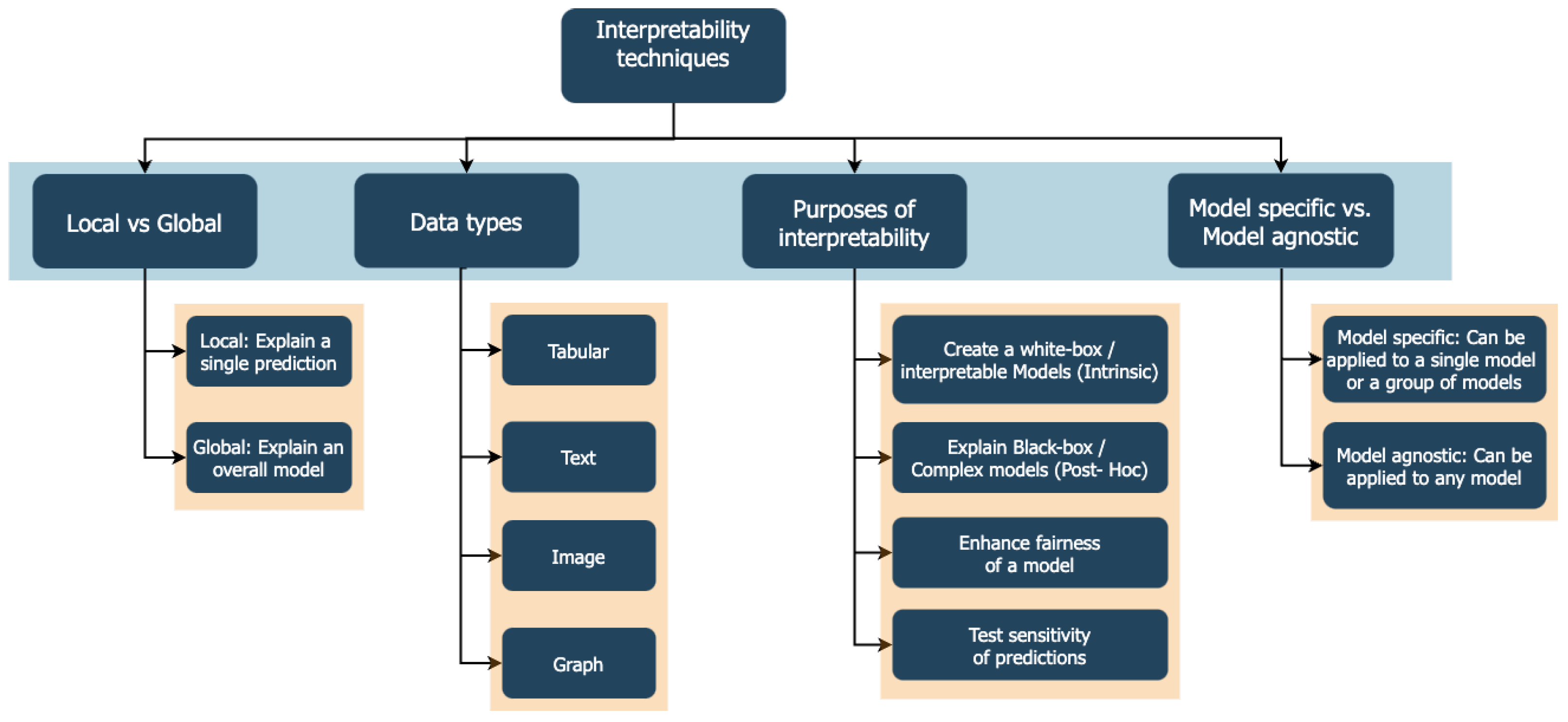
3.2. Interpretability Techniques

Interpretability techniques are methods used to understand and interpret the behavior and decisions of machine learning models [43]. They are the process or approach used to uncover the underlying logic and reasoning of a model’s predictions or classifications. Figure 1 describes a broad classification of some of these techniques.

We describe some of the important techniques that are used to understand or achieve interpretability from Figure 1.

• Local interpretation: An interpretation of a single data point is called a local interpretation. For example, why does a model predict that a particular borrower would default? This is an example of a local interpretation.
• Global interpretation: This provides an overall understanding of how a model makes decisions across all instances. It helps to understand the model’s behavior in a broader sense, making it easier to grasp the underlying patterns or features that the model uses for its decisions.
• Intrinsic explanation: This technique involves inherently interpretable models, such as linear regression or decision trees, where the decision-making process is transparent and directly understandable. Hence, there is no need for any post-analysis.
• Post-hoc explanation: This technique explains ML models after training. It is used to interpret complex models like neural networks which are not intrinsically interpretable. It extracts correlations between features and predictions.
• Model-specific: It is tailored to specific types of models, leveraging their unique structures and properties for interpretation, such as feature importance in random forests.
• Model agnostic: Model-agnostic methods can be applied to any machine learning model, regardless of its internal workings, providing flexibility in interpreting various types of models without needing to understand their specifics.

3.3. Limitations of XAI

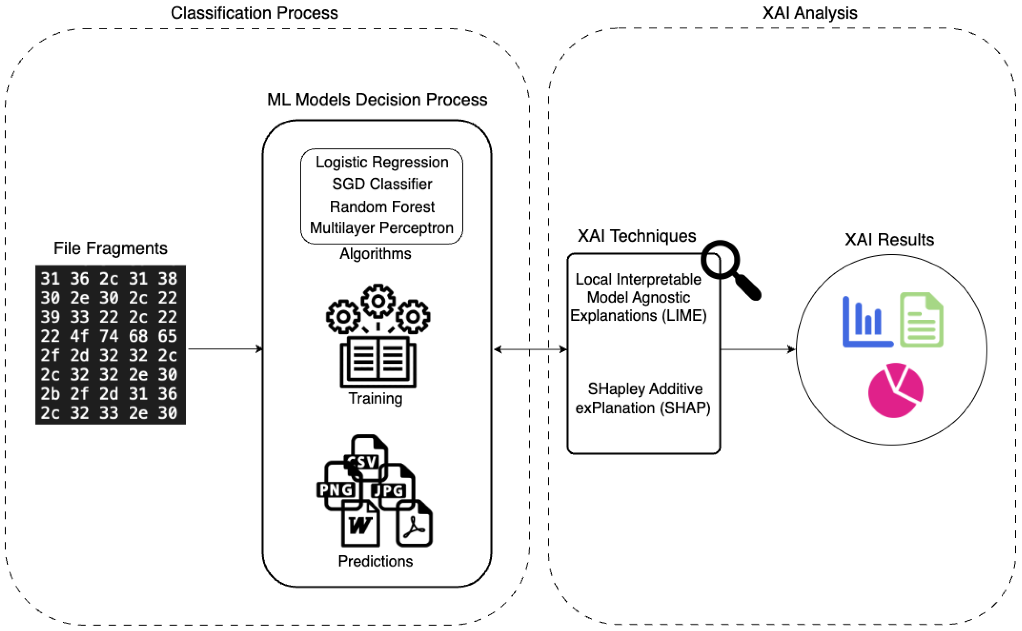
Generally, most machine learning algorithms focus primarily on minimizing a loss function, rather than making the models easy to interpret, understand, or create. The models try to reduce the difference between their predictions and the actual outcomes. This process aims to make the models’ predictions as accurate as possible on the given data, hoping that it will also perform well on new, unseen data. Therefore, XAI only attempts to explain why the model generates the predictions it carries out. Since XAI provides us with effect sizes (impact of variables), it is tempting and wrong to give them a causal interpretation. Hence, XAI tools are valuable for understanding model behavior and correlations, but causality should be established through careful research and experimentation.

For example, a model that predicts the cost of a house based on its size of land, its location, and the presence of a swimming pool. Using eXplainable AI (XAI) tools, as illustrated in Figure 2, we can understand how important each of these variables is and the effect of each variable in generating each prediction. However, these tools do not tell us why some houses are more expensive than others, they merely explain how the predictions were generated. We might find that the model estimates the highest house prices belong to large houses in upscale neighborhoods with swimming pools. The reason why the model estimates that these houses have the highest prices is that houses fitting that description in the dataset were mostly luxury mansions in exclusive neighborhoods with many amenities, and predicting a high cost for these house types minimized the loss function we selected. There is no causal relationship between, for example, having a swimming pool and the cost of a house. It is an observed correlation in the dataset. If we observe additional variables like “number of bedrooms” or “proximity to the city center”, we might rightly attribute a causal effect between those variables and house prices. However, the model itself does not inherently understand the reasons or causal relationships; it learns from patterns in the data, which may not represent real-world causality.

Another possible disadvantage of XAI can come from its criminal or unethical usage. XAI models can reveal the inner workings of ML models and provide us with a better understanding; however, there are some times when models should only be made transparent to a limited number of people. Open and transparent models can be open to exploration or being gamed by unauthorized users. As an example, if a search engine’s algorithm was open to everyone, the recommended websites at the top of each query would likely just be those that best exploited the model, not the websites people generally want to visit. For self-driving cars, a cybercriminal could trick the AI powering the car into having an accident.

4. Methodology

This research aims to apply XAI techniques to machine learning models used for file fragment classification. File fragment analysis is a crucial task in various contexts, including network file analysis, malware analysis, and developing software for data retrieval from unknown or malfunctioning software. Each of these tasks requires specific approaches to effectively analyze and classify file types. For this research, we focus on the classification of file fragments using Byte frequency analysis(BFA), machine learning, and explainable AI (XAI) techniques. While our primary aim is to enhance the interpretability and reliability of file fragment classification, the insights gained from our methods can also contribute to these broader contexts by providing a deeper understanding of the data structure and the decision-making processes of classification models.

By applying explainable AI techniques to these machine learning models, we can uncover the underlying factors that influence their predictions and gain insights into their decision-making process. This can be achieved by using various interpretability methods such as feature importance analysis, rule extraction, or visualizations to understand the patterns and rules learned by the models. Through this analysis, we can identify the key features or attributes that contribute to the classification decisions made by the models. Understanding these features and attributes will help further research into files and their compositions. For our analysis, we use various XAI techniques to analyze and understand the models used in the research. Figure 3 describes the proposed model for the analysis.

In this research, we iterate the Byte Frequency Analysis (BFA) technique and classification process across three file sizes: 512 bytes, 1024 bytes, and the entire file fragment. The initial step involves removing the header and footer byte content in the files. We then randomly select 512, 1024, or the remaining bytes before applying the BFA technique.

Formally, let F represent the file fragments, and let B denote the set of all possible byte values, where $B=\{0,1,2,\dots ,255\}$. For a given file fragment F, the BFA technique involves calculating the frequency of each byte value $b\in B$. This can be represented as a frequency vector $\mathbf{f}\left(F\right)=[f_0,f_1,\dots ,f_{255}]$, where $f_b$ denotes the frequency of byte b in fragment F.

During preprocessing, we normalize these frequency vectors to standardize feature scales. Let $\mathbf{n}\left(F\right)$ be the normalized frequency vector, computed as:

$$\mathbf{n}\left(F\right)=\frac{\mathbf{f}\left(F\right)}{{\parallel \mathbf{f}\left(F\right)\parallel }_2}$$

where ${\parallel \mathbf{f}\left(F\right)\parallel }_2$ is the Euclidean norm of the frequency vector.

To address dataset imbalances, we apply the Synthetic Minority Over-sampling Technique (SMOTE). This technique generates synthetic samples for the minority class by interpolating between existing samples. Let $S_{\mathrm{minority}}$ be the set of minority class samples. For each sample $s\in S_{\mathrm{minority}}$, a synthetic sample $s^{\prime }$ is generated as:

$$s^{\prime }=s+\lambda (s_{\mathrm{nearest}}-s)$$

where $s_{\mathrm{nearest}}$ is the nearest neighbor of s in the feature space, and $\lambda$ is a random number between 0 and 1.

The preprocessed data, consisting of normalized frequency vectors and SMOTE-generated samples, is then used as input for our machine learning models. Let $\mathbf{X}$ be the matrix of input features, where each row represents a normalized frequency vector $\mathbf{n}\left(F\right)$, and let $\mathbf{y}$ be the corresponding labels indicating the file type.

We train various machine learning models, denoted as ${\mathcal{M}}_1,{\mathcal{M}}_2,\dots ,{\mathcal{M}}_k$, on the dataset $(\mathbf{X},\mathbf{y})$. Each model ${\mathcal{M}}_i$ maps the input feature vectors to predicted labels: ${\widehat{\mathbf{y}}}_i={\mathcal{M}}_i\left(\mathbf{X}\right)$.

To interpret the predictions made by these models, we employ Explainable Artificial Intelligence (XAI) techniques, specifically Shapley Additive Explanations (SHAP) and Local Interpretable Model-Agnostic Explanations (LIME). These techniques provide insights into the contribution of each feature (byte frequency) to the model’s predictions. Let $\Phi$ denote the SHAP values, and $\mathcal{L}$ denote the LIME explanations. For a given model ${\mathcal{M}}_i$ and an input $\mathbf{x}\in \mathbf{X}$, the SHAP values ${\Phi }_i\left(\mathbf{x}\right)$ and LIME explanations ${\mathcal{L}}_i\left(\mathbf{x}\right)$ are computed as:

$${\Phi }_i\left(\mathbf{x}\right)=[{\varphi }_0,{\varphi }_1,\dots ,{\varphi }_{255}]$$

$${\mathcal{L}}_i\left(\mathbf{x}\right)=[l_0,l_1,\dots ,l_{255}]$$

where ${\varphi }_b$ and $l_b$ represent the contribution of byte value b to the prediction for input $\mathbf{x}$.

These interpretations allow us to validate and understand the decision-making process of our models, enhancing transparency and trust in the classification of file fragments.

The model consists of two major entities that are used to understand and explain the decisions and predictions of the machine learning models used in the previous research. The entities are the classification process and the XAI analysis. The first entity includes the data preprocessing, model training, and prediction while the second entity involves analyzing the prediction made in the first.

4.1. Classification Process

The classification process encompasses the previous work [1] which focuses on data preparation, model training, and prediction. We apply the Byte Frequency Analysis (BFA) technique to these fragments to capture the frequency of each byte value, creating a feature set that reflects the underlying binary data structure. This approach allows our machine learning models to effectively learn and classify different types of files based on their binary characteristics.

4.1.1. Dataset

The dataset utilized in our previous research [1] comprises fourteen distinct file types: jpg, png, csv, doc, gif, gz, html, log, pdf, ppt, ps, txt, xls, and xml. These file types were chosen due to their prevalence in forensic investigations and their frequent appearance in prior studies. This selection encompasses a broad spectrum of content, formats, and sizes, ensuring the introduction of variability essential for comprehensive experimentation. From the previous research, we had 14 classes representing the different file types that were used. The dataset was obtained from DigitalCorpora.org [45], which is a publicly available digital corpus repository for computer forensics education and research. The dataset consists of over 15,000 files. File types and their associated numbers and labels are shown in

Table 1. Description of Dataset.

File Type	Class Label	Number of Files
csv	Class 0	179
doc	Class 1	1102
gif	Class 2	424
gz	Class 3	127
html	Class 4	3839
jpg	Class 5	937
log	Class 6	110
pdf	Class 7	3766
png	Class 8	88
ppt	Class 9	892
ps	Class 10	254
txt	Class 11	3224
xls	Class 12	667
xml	Class 13	188

.

4.1.2. Machine Learning Models

In the previous research [1], we used various machine learning models to predict the file types of file fragments. The experiment used two distinct analysis types which are Byte Frequency Analysis (BFA) and grayscale imaging. However, in this research, we focus only on the BFA analysis and its classification models. We focus on the BFA analysis and result due to its better performance. BFA is a technique used in cybersecurity and digital forensics to analyze the distribution of byte values within a file or its fragments. Byte frequency analysis involves examining the occurrences and patterns of these byte values within a given file. Assessing the distribution of byte values can give insights into the file’s structure, identify potential file types, and detect anomalies or malicious content. Each byte is represented by an 8-bit binary number, allowing for 256 possible values (0 to 255). which is represented by its corresponding hexadecimal value. During the analysis, the frequency of each byte value is recorded and this is used as the input or the machine learning models. Additionally, the byte content is analyzed only using unigrams. In the unigram analysis, the frequency of each byte is found by taking bytes as single values. As a result, there are 256 possible values or features per byte ($2^8=256$).

In the experiment, we iterate the BFA technique and classification process across three file sizes, which are 512 bytes, 1024 bytes, and the entire file fragment. The first process was to remove the header and footer byte content in the files. We then randomly select 512, 1024, or the remaining bytes before applying the BFA technique. Before classification, we conduct feature normalization during preprocessing to standardize feature scales and expedite experiment runtime. Additionally, we utilize the Synthetic Minority Over-sampling Technique (SMOTE) to rectify dataset imbalances and mitigate bias. This preprocessed data is subsequently fed into our classification models. These models were then evaluated using several metrics, including accuracy, precision, recall, and F1-score, to assess their performance comprehensively. The performance of each model was analyzed and compared to determine which model best predicts the file types of the fragments. However, for this research, we only focused on the models for the entire fragment as this gave us the best result.

4.2. XAI Analysis

The second stage of the proposed model is the analysis of the decision-making process of the machine learning models. This is the focus of this research. We employ two XAI techniques which are SHAP and LIME. We use these models because they are both model-agnostic, which means they can be easily applied to many machine learning models regardless of their underlying architecture or complexity. This allows us to apply these models to the different ML models used in the study. In addition, LIME focuses on local interpretability by generating explanations for individual predictions. This emphasis on local interpretability makes it particularly valuable for gaining insights into the decision-making process for individual file fragments, contributing to the transparency of the classification outcomes. Furthermore, SHAP provides both local and global views of feature importance and the impact of each feature on the overall model predictions. Global interpretability is beneficial for identifying key features that consistently influence the classification results across the entire dataset. This can reveal overarching patterns and contribute to a deeper understanding of the critical features contributing to the classification decisions. Overall, LIME and SHAP offer complementary insights into the entire machine learning models’ behavior and decision-making. LIME excels in providing fine-grained, instance-specific explanations, while SHAP provides a more holistic view of feature importance. By using both techniques, we aim to offer a comprehensive and nuanced understanding of how machine learning models make their decisions.

4.2.1. Local Interpretable Model Agnostic Explanations

Local Interpretable Model Agnostic Explanations, popularly known as LIME [10], is a model agnostic interpretability technique. It treats machine learning models as black-box algorithms and only has access to the outputs of the model. That is, LIME does not require any information about the model’s parameters. For example, LIME does not need to know the architecture of a neural network, its weights, or activation values. It is defined as

$$LIME(\widehat{f})=\arg \underset{g}{\min }\mathcal{L}(f,g,{\pi }_x)+\Omega \left(g\right)$$

where $LIME(\widehat{f})$ is the technique for generating local, interpretable explanations for a complex machine learning model. It aims to provide insights into the decision-making process of the model for a specific data instance. $\arg \underset{g}{\min }$ represents an optimization process. It seeks to find the model g that minimizes the value of the expression that follows, subject to certain constraints. $\mathcal{L}(f,g,{\pi }_x)$ is the loss function $\mathcal{L}$ which measures the difference or loss between the predictions of the original model f and the explanation model g for the specific data instance x. The goal is to minimize this loss, meaning g should provide predictions that closely match f for x. $\Omega \left(g\right)$ represents the complexity penalty associated with the explanation model g. It discourages overly complex explanation models. The penalty term can take various forms, such as L1 or L2 regularization, to ensure that the explanation model is simple and interpretable.

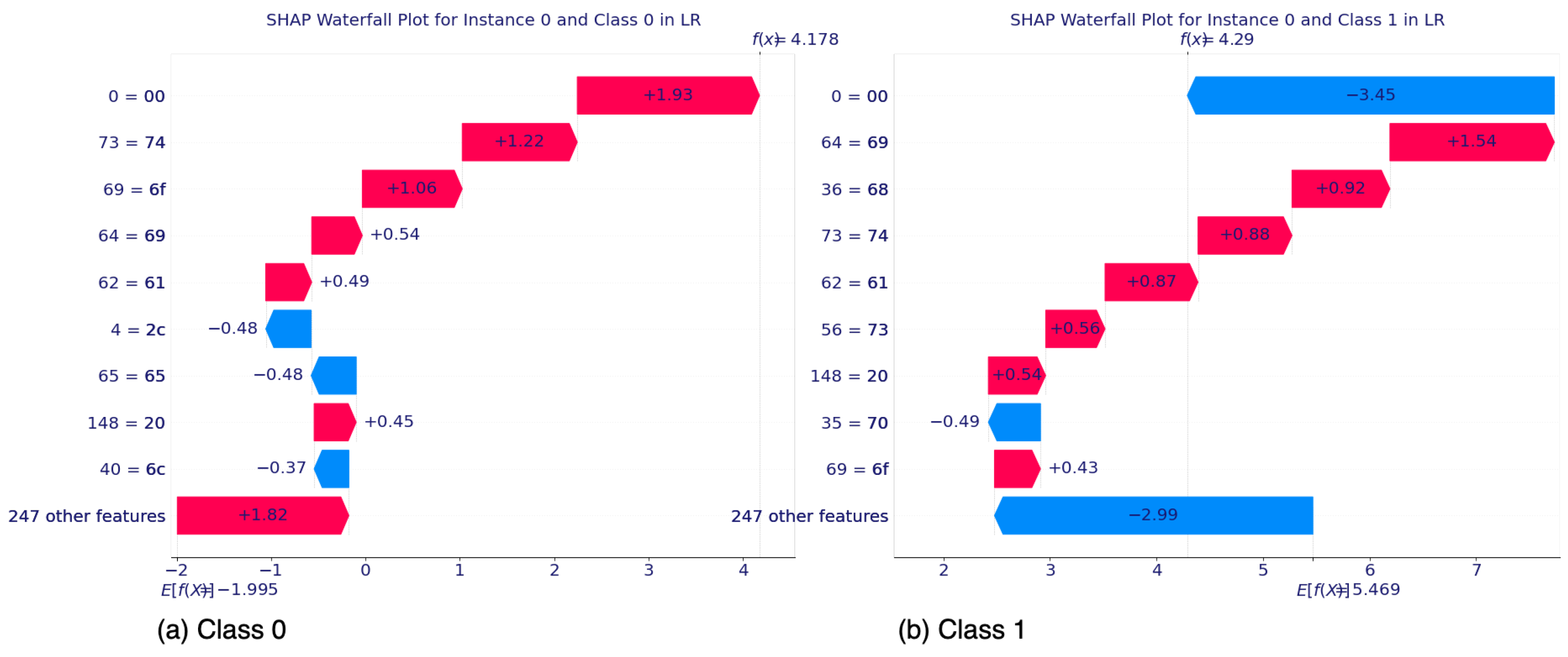
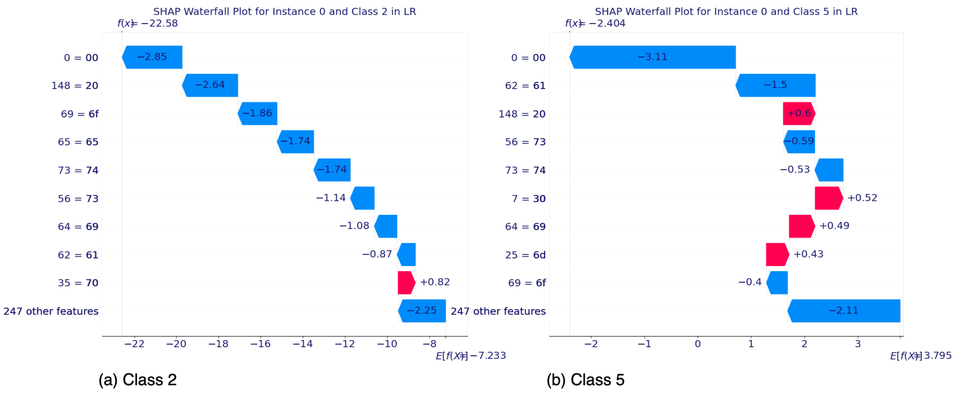
4.2.2. SHapley Additive exPlanation

SHAP (Shapley Additive Explanations) [9] is an advanced and versatile technique in Explainable Artificial Intelligence (XAI) used to explain the predictions of machine learning models. It provides a unified framework for understanding the contributions of individual features or factors to a model’s predictions. SHAP values are based on cooperative game theory concepts, specifically Shapley values, which originate from the field of economics. SHAP values is represented as

$${\varphi }_i\left(f\right)=\sum _{S\subseteq N\setminus \left\{i\right\}}\left(\frac{\left|S\right|!·\left(\right|N|-|S|-1)!}{\left|N\right|!}\right)\left[f(S\cup \{i\left\}\right)-f\left(S\right)\right]$$

where ${\varphi }_i\left(f\right)$ represents the SHAP value for feature i in the context of the model f. SHAP values explain how much each feature contributes to the model’s prediction. N denotes the set of all features (input variables) in the model while S is a subset of features from N (excluding feature i). $\left|S\right|$ is the number of features in the subset S and $\left|N\right|$ the total number of features in N. $f(S\cup \{i\left\}\right)$ represents the model’s prediction when all features in subset S are included along with feature i. $f\left(S\right)$ is the model’s prediction when only features in subset S are considered (excluding feature i).

The SHAP value for a feature i measures how much adding feature i to a given subset of features (S) changes the model’s prediction. It calculates the marginal contribution of feature i to the prediction, taking into account all possible combinations of features. The formula embodies the principle of “fairness”, ensuring that each feature’s contribution is fairly attributed to the model’s prediction, much like in cooperative game theory where the Shapley value assigns fair contributions to each player in a cooperative game. SHAP values can be applied to a wide range of machine learning models, making them a valuable tool for understanding model behavior, feature importance, and decision explanations. They are particularly useful for model interpretability and transparency, helping practitioners, researchers, and data scientists comprehend why a model produces specific predictions.

5. Experimental Result and Analysis

In this section, we describe the experimental setup and results of the research. The setup is described for reproducibility and validity. Next, we visualize and analyze the results of the experiment to gain insights and understand the models’ predictions.

5.1. Experimental Setup

The experimental setup is crucial in our interpretability research as it ensures the reproducibility and validity of the results and findings. It describes the hardware and software configuration that is used to implement the experiments. For the hardware configuration, the system featured a workstation with 80 GB of RAM, an Intel Core i7 processor, and an NVIDIA GeForce RTX 3080 GPU to accommodate the computational demands of training the deep learning model and implementing the XAI libraries. For the software setup, all experiments were conducted within a Jupyter Notebook environment, facilitating transparent documentation and code reproducibility. The primary programming language for our experiment is the Python version 3.10.14. For the XAI experiments, we used LIME version 0.2.0.1 and SHAP version 0.43.0.

5.2. Results

To simplify and concisely summarize our research efforts, we limit our analysis to four of the nine models in the previous study [1]. The models analyzed are Logistic Regression (LR), Random Forest (RF), Stochastic Gradient Descent (SGD), and Multilayer Perceptron (MLP) models. The models’ performances for file classification from the previous research are described in

Table 2. Results of models.

	Precision	Recall	F1-Score	Accuracy
Logistic Regression	0.63	0.40	0.44	0.40
SGD Classifier	0.71	0.36	0.36	0.36
Random Forest	0.59	0.51	0.46	0.51
MultiLayer Perceptron	0.92	0.89	0.89	0.89

.

The interpretability analysis of the experiment encompasses both global and local explanations. SHAP values were computed for feature attribution, offering insights into the relative importance of the byte features in predictions. SHAP provides a global perspective, offering a unified framework for feature attribution. The SHAP summary plot vividly displayed the impact of each feature on classification outcomes. In the plot, we observe the specific byte content that significantly influenced the model’s predictions. Furthermore, we use the SHAP waterfall plot to visualize individual predictions, providing a clear breakdown of the contributions of each feature to particular classifications. This enables us to identify critical patterns and associations in the data.

We use LIME to complement the visualization of our analysis. LIME generates localized insights into the models’ behaviors. LIME generated explanations for individual file fragment classifications, making each model’s decision-making transparent and understandable. The LIME explanations allow us to pinpoint the presence of specific features that played a decisive role in the models’ classifications. These explanations enhanced our understanding of the model and also provided actionable insights for refining the classification process.

For our experiments and analysis, the application of SHAP for the models details global and local interpretability. Local interpretability explains predictions for individual instances of the dataset. SHAP explains how individual predictions are arrived at in terms of contributions from each of the model’s input variables. We use SHAP’s waterfall plot to explain the local interpretability. Waterfall plots show the most complete detail of a single prediction. Alternatively, global interpretability describes the expected behavior of machine learning models concerning the whole distribution of values for its input variables. We use both bar and beeswarm plots for the global analysis. The bar plot gives a quick summary of the mean absolute SHAP value for each feature across all of the data. We also utilize beeswarm plots as they are more complex and detailed as they reveal not just the relative importance of features, but their actual relationships with the predicted outcome.

Overall, the combined application of SHAP and LIME offered a holistic view of our models’ performances, enhancing their interpretability and transparency. The visualizations and explanations enabled us to discern the significance of different features and understand how they contributed to the classification of file fragments, ultimately advancing the effectiveness of our file fragment classification system.

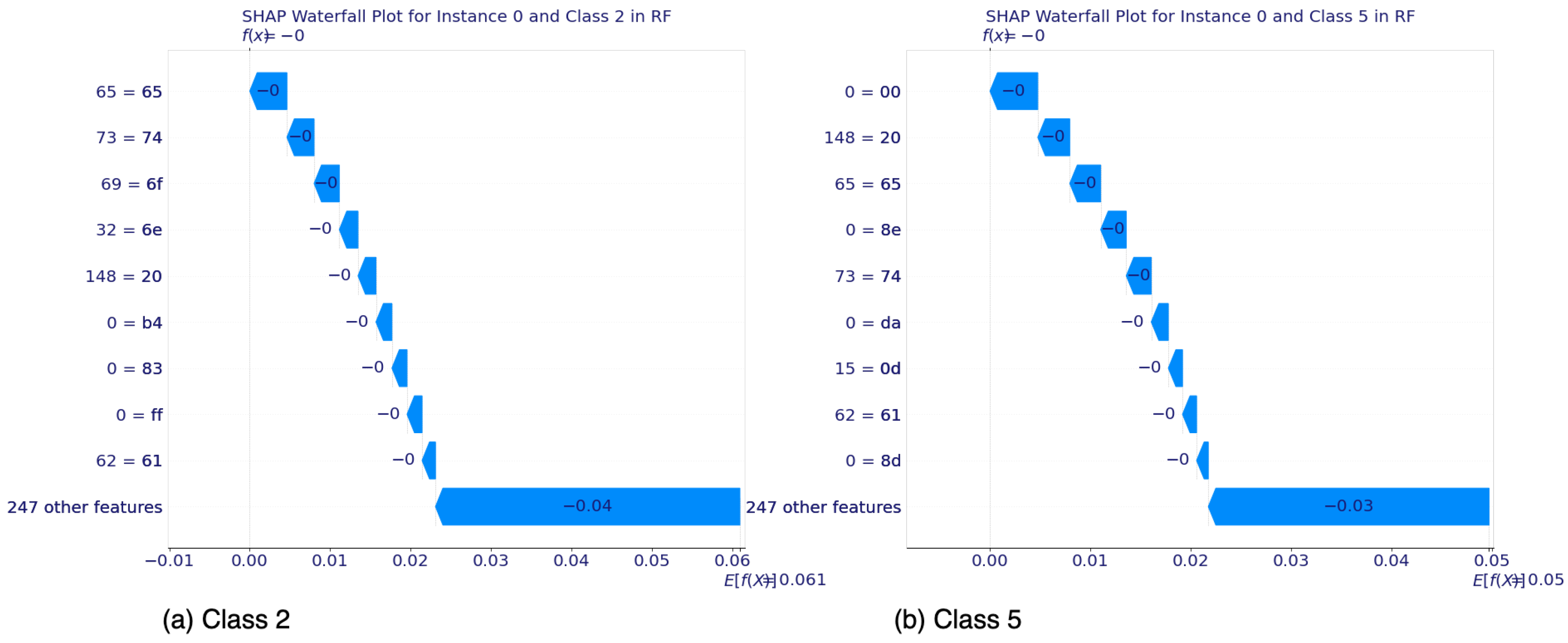
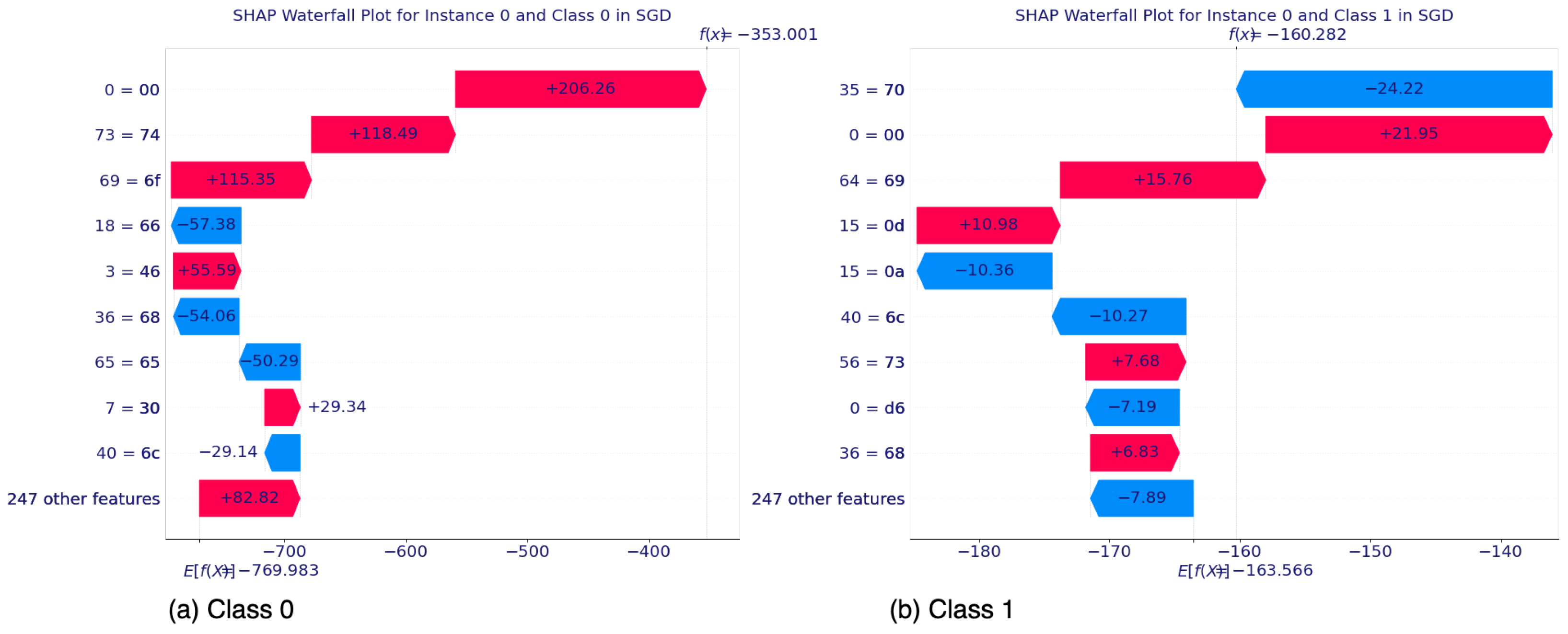
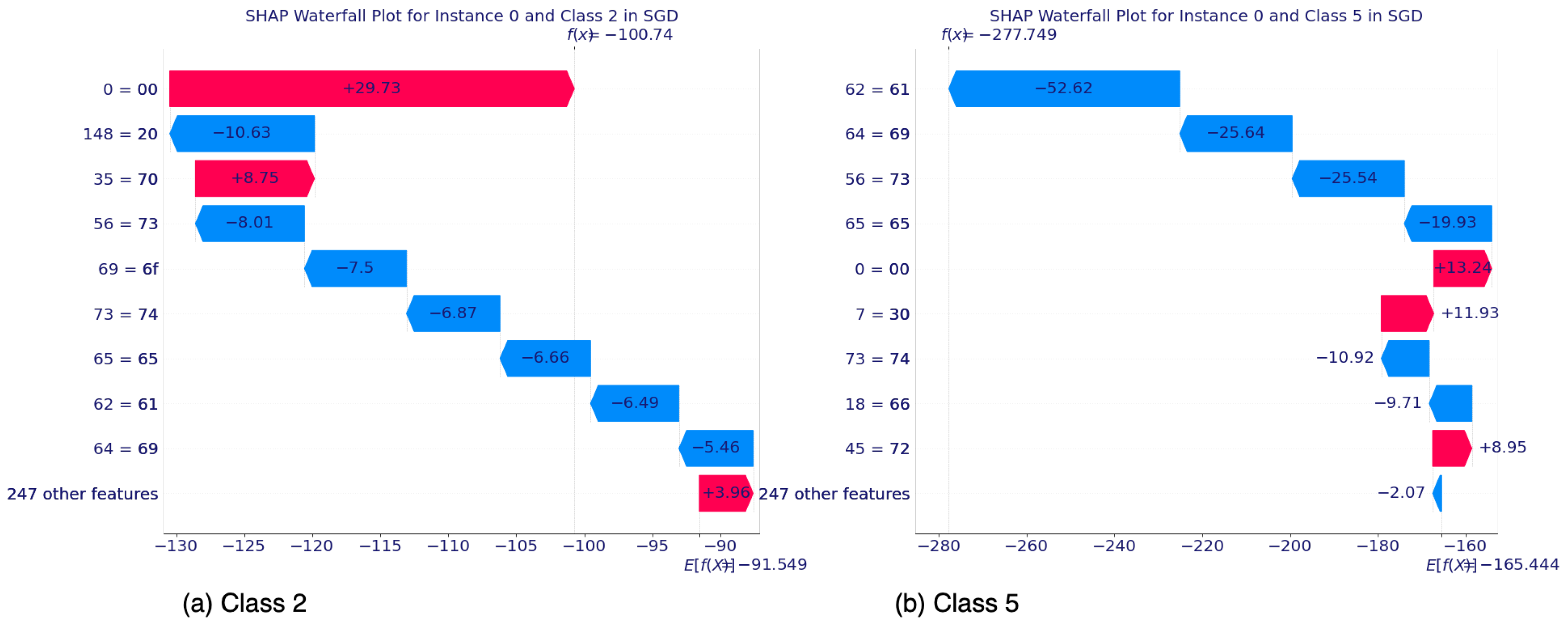
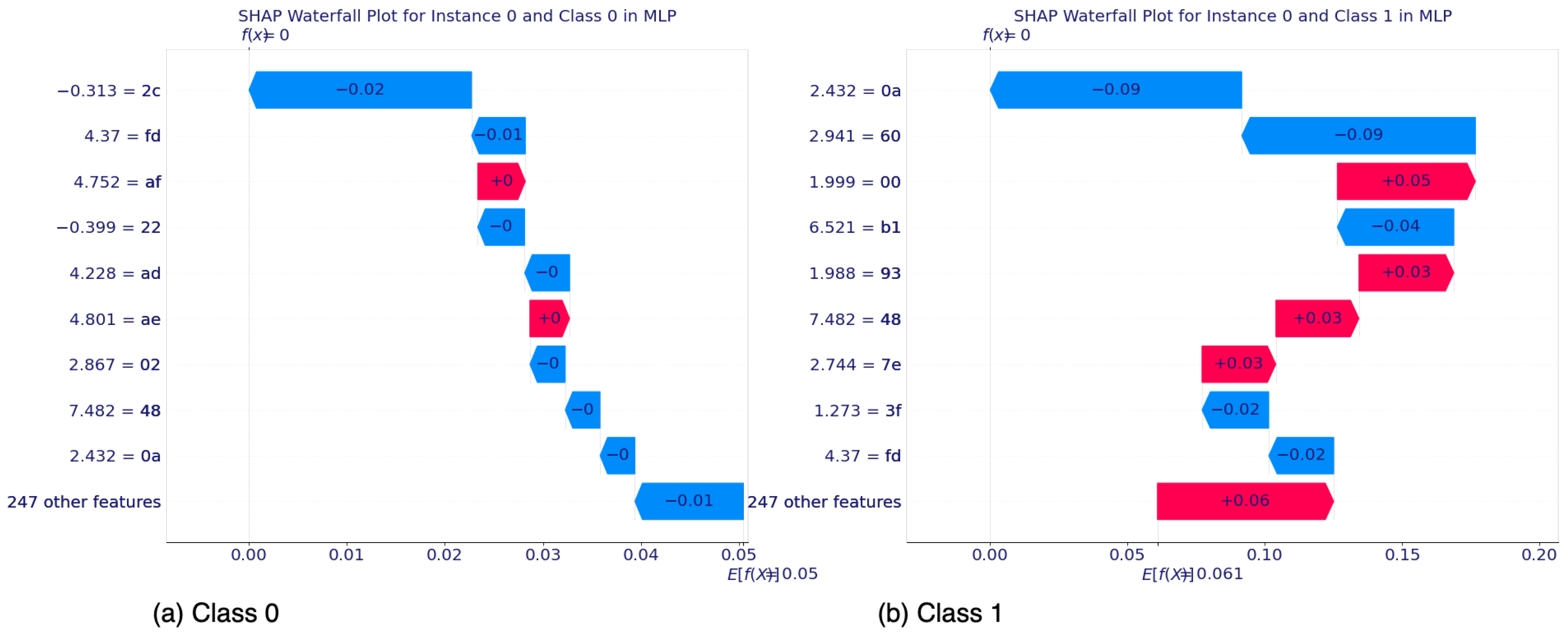
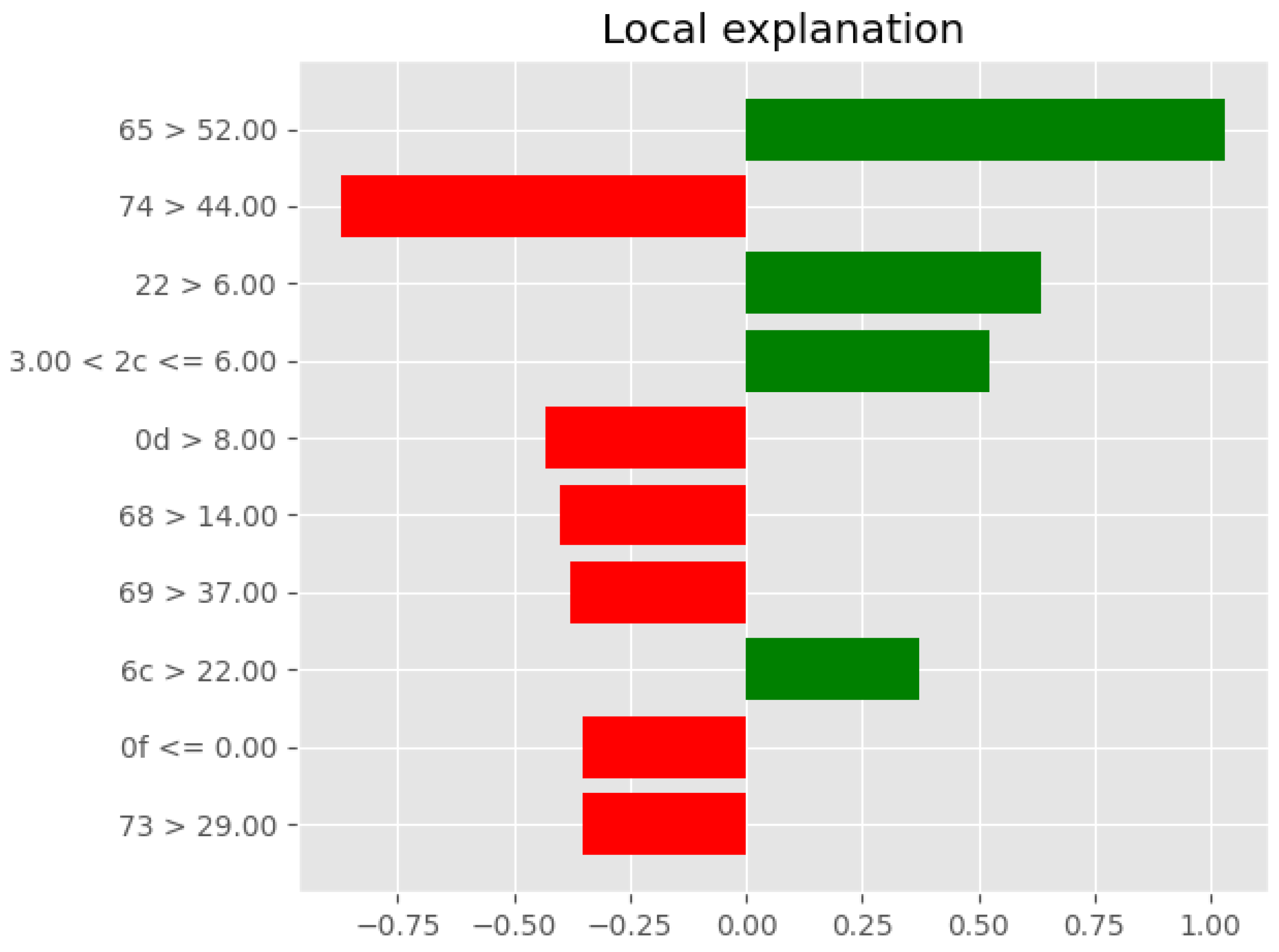
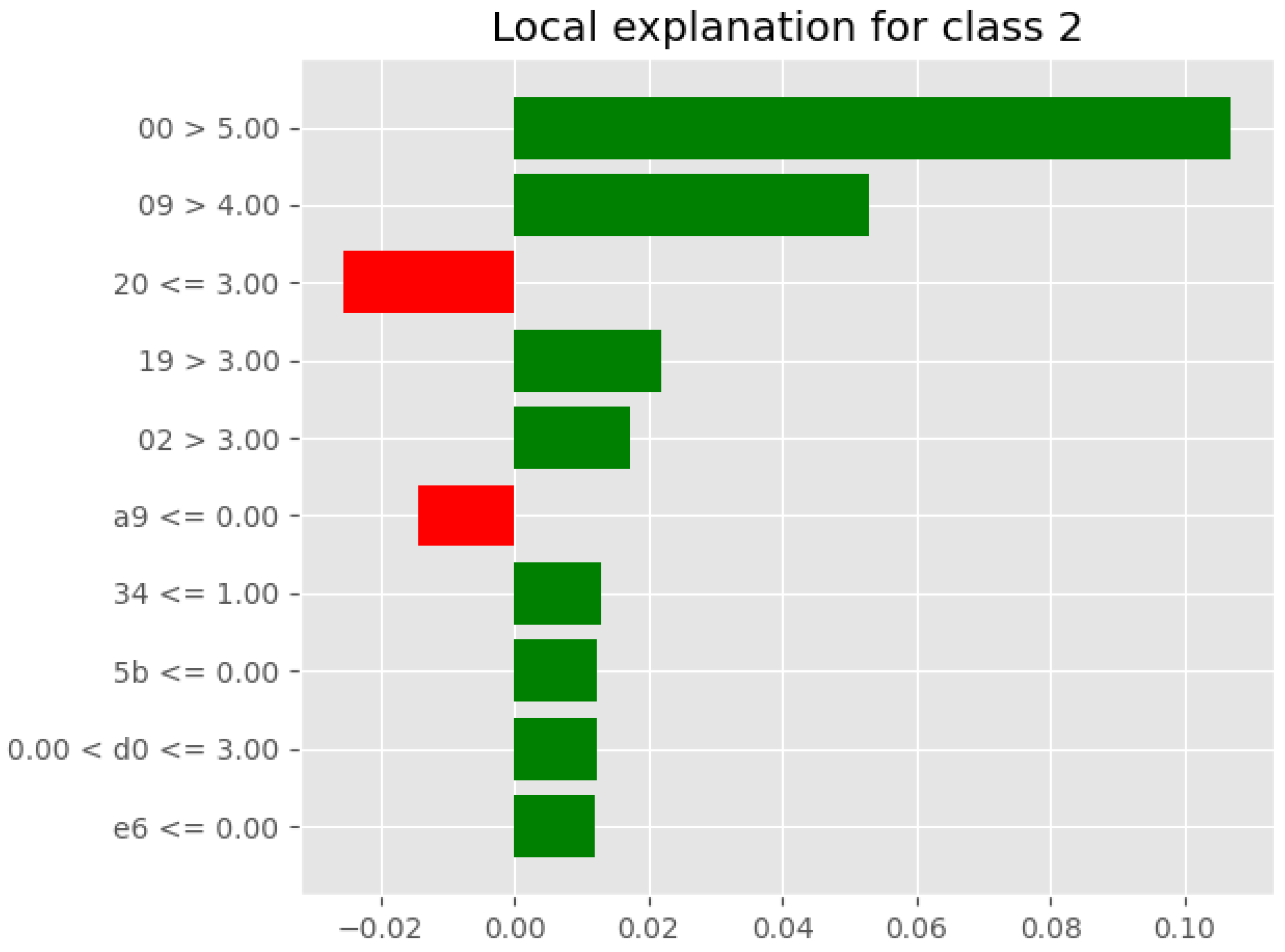
5.2.1. SHAP’s Local Interpretability

The integration of SHAP techniques into our machine learning model for file fragment classification yielded profound insights into the model’s decision-making process. For the local interpretability analysis, we use the waterfall plot. The waterfall plot gives a detailed explanation of how each byte content contributes to the predicted file type for each instance of the data.

The waterfall plot starts from the baseline prediction and visually shows how the addition or removal of each feature influences the model’s prediction. Positive contributions which are color-coded red are depicted as bars that push the prediction higher, while negative contributions (in blue color) are represented as bars that pull the prediction lower. The length and direction of the bars in the plot provide valuable insights into the influence of each feature on the model’s decision-making process.

The x-axis of a SHAP waterfall plot represents the SHAP value, which quantifies the contribution of each feature to the model’s prediction. The y-axis lists the features ordered by the magnitude of their SHAP values for the chosen test instance. To reduce clutter and focus on the most impactful features, the most impactful features are shown (top nine in our research), and the remaining features are aggregated into a single entry.

Furthermore, the waterfall plot shows ‘$E\left[f\right(X\left)\right]$ and $f\left(x\right)$’ markers. $E\left[f\right(X\left)\right]$ marker stands for the expected value of the model’s output for a given class based on the average across the dataset while $f\left(x\right)$ called the final predicted value is the sum of the expected value and all the feature contributions. It indicates the final output for the instance after all feature contributions have been accounted for.

Figure 4a,b and Figure 5a,b show the logistic regression’s waterfall plots for the chosen test instance with Classes 0, 1, 2, and 5, respectively. The LR model predicted the output as Class 5, hence its inclusion.

In the LR analysis, we use a test instance that was predicted to belong to Class 5 (jpg file type) by the model. Figure 4 and Figure 5 describe the contributions of individual features to the model’s prediction for the test Instance, across Classes 0, 1, 2, and 5.

Specifically, Figure 4a illustrates the model’s expected log odds output ($E\left[f\right(X\left)\right]$) for Class 0 which starts at −1.995. Features such as ‘00’ and ‘6F’ contribute positively to the log odds of the prediction, while features ‘6C’ and ‘2C’ contribute to lowering the prediction log odds. The combined effect of these contributions leads to a final predicted log odds ($f\left(x\right)$) of 4.178. The positive shift from the expected value suggests that the presence of specific byte frequencies is associated with an increased likelihood of this instance being classified in Class 0. Likewise, Figure 5b which represents Class 5 (the predicted output) shows an expected log odds output as 3.795, with the features ‘00’, ‘61’, ‘20’, and ‘6F’ contributing negatively, while ‘30’, ‘69’, ‘6D’, and ‘other features’ contribute positively. The final predicted log odds of −2.404 indicate a shift from a positive association with Class 5 based on the expected value to a negative association. The model, therefore, predicts Class 5 with less certainty than initially expected based on the mean log odds.

Generally, across all classes, the byte ‘00’ consistently appears to be an influential feature. For Class 0, the feature ‘00’ positively impacts the model’s prediction, increasing the log odds. Conversely, for Class 2 (Figure 5a), the same feature ‘00’ contributes negatively. This shows how the same feature can have a different impact depending on the class context. In Figure 4a,b, representing Classes 0 and 1, respectively, feature ‘6F’ contributes positively to the model’s prediction. The consistent positive contribution in these classes could indicate a specific byte frequency that is characteristic of these classes in the dataset. The ‘247 other features’ entry in the plots indicates a collective contribution from the remaining features. In Class 0 (Figure 4a), the aggregated features contribute positively, whereas, in Class 2 (Figure 5a), they have a negative impact.

Another insightful detail is the prediction for the LR model for the test instance. The model predicted the instance as belonging to Class 5. We see that many features contribute negatively which moves the final prediction value to negative from an expected positive value. This means that the model has a likelihood to predict Class 5 (due to the positive expected value), however, the specific features of the instance reduced that likelihood (hence the negative final value). Despite this decrease, Class 5 was predicted and this can be attributed to other factors.

For the RF analysis, we analyze the same test instance as the LR model. Figure 6a,b and Figure 7a,b show the RF’s waterfall plots for the chosen test instance with Classes 0, 1, 2, and 5, respectively. Like the LR model, the RF model also predicted the output as Class 5.

Generally, the SHAP values in the waterfall plots for the RF model appear to be quite small, with many features contributing either negligible or zero impact indicated by “−0” in the plots. This can be interpreted as approximately zero or a very small number rounded to zero. This means that the RF model is finding no strong evidence for the instance from most of the individual features to shift the prediction away from the base rate prediction for these classes.

For Classes 0 and 1, the expected values $E\left[f\right(X\left)\right]$ start effectively at zero. The contributions of individual features are minimal, close to zero, which results in final predicted log odds $f\left(x\right)$ that are very close to the expected value. This suggests that for the test instance, the RF model finds almost no evidence within the features to push the prediction toward or away from these classes. Class 2 has a final predicted log odds of −0.061 which indicates a slight shift away from the base rate prediction toward a negative association with Class 2. However, this shift is very small and suggests weak evidence against Class 2 for the test instance. Similar to Class 2, Class 5 has a final predicted log odds of −0.03. This indicates a weak negative association with Class 5 for Test Instance 0.

In summary, the waterfall plots for the RF model on the test instance suggest that the model’s predictions are based on the aggregate influence of a large number of features, each contributing a minor effect. The lack of strong individual feature contributions indicates that the model may be relying on subtle, complex interactions between features to make predictions. This pattern of prediction could suggest that the model is quite sensitive to small changes in feature values and that the feature space for the classification task is highly dimensional with intricate decision boundaries.

The waterfall plot results for the SGD model are visualized in Figure 8 through Figure 9.

Similar to both LR and RF models, SGD also predicted the same test instance as Class 5. Features ‘00’, ‘69’, ‘73’, and ‘62’ appear across multiple classes, indicating their overall importance in the model’s decision process. The impact direction of these features, however, varies across different classes, which highlights the complexity of the classification task and the classifier’s sensitivity to the context provided by the combination of features. Also, the plots demonstrate that certain features can have a large magnitude of impact, both positively and negatively. Features (‘00’ and ‘69’) that consistently have a large magnitude across classes can be considered key features that the model heavily relies on for making predictions. Furthermore, the balance between positive and negative contributions can provide insights into the classifier’s certainty. For instance, Class 0 shows a strong positive shift indicating high certainty, whereas Class 1 and Class 5 have a negative shift, reflecting lower certainty or confidence in association with these classes.

Although the final predicted value for Class 5 is negative, suggesting a weaker association with Class 5, the classifier still predicts this class. This indicates that for the SGD classifier, while the SHAP values for the test instance relative to Class 5 are not strongly positive, they may be comparatively less negative than for other classes, leading to the prediction of Class 5. The SHAP Waterfall plots for the SGD classifier reveal intricate patterns of feature influence, with certain features playing pivotal roles across classes. The varying magnitudes and directions of these contributions underscore the classifier’s nuanced interpretation of the input features. Despite some negative final predicted values, the model may still favor certain classes if these values are the least negative among all classes, reflecting the comparative nature of the decision-making process in a multi-class setting. The plots underscore the importance of understanding both individual feature impacts and their collective influence to appreciate the model’s predictions fully.

Due to resource constraints, we use a test instance different from the other models for the MLP analysis. Figure 10a,b and Figure 11a,b show the plots for Classes 0, 1, 2, and 8, respectively.

Feature ‘FD’ appears in most of the classes with a consistently negative contribution, suggesting it may be a key feature in the model’s prediction across multiple classes. The fact that it contributes negatively in each class could point to its general importance in the dataset or a specific interaction with test instance 0 that the MLP model finds predictive. The magnitude of feature contributions varies significantly across classes, with some features having a much larger impact on certain classes (‘49’ and ‘4F’ for Class 0) than others. This variation in feature importance across classes is indicative of the classifier’s ability to differentiate between classes based on the presence and strength of certain features.

The SHAP Waterfall plots for the MLP classifier underscore the significance of individual features and their collective influence on the predictive outcomes for Test Instance 0. The variability in the direction and magnitude of feature contributions across different classes captures the complexity of the classifier’s decision-making process and emphasizes the importance of understanding these feature-level dynamics for model interpretation. These insights are integral to validating the model’s performance, guiding feature engineering efforts, and enhancing transparency in machine learning applications.

Across all four models, features ‘00’ and ‘4F’ appear to have a notable impact across the models and classes. This could suggest that these features are key indicators within the dataset, regardless of the model. In the plots, the entry labeled ‘247 other features’ is an aggregation of the remaining features. In some of the plots where this aggregated contribution is consistently positive or negative across models, it could suggest that many weak signals combine to have a more substantial cumulative impact.

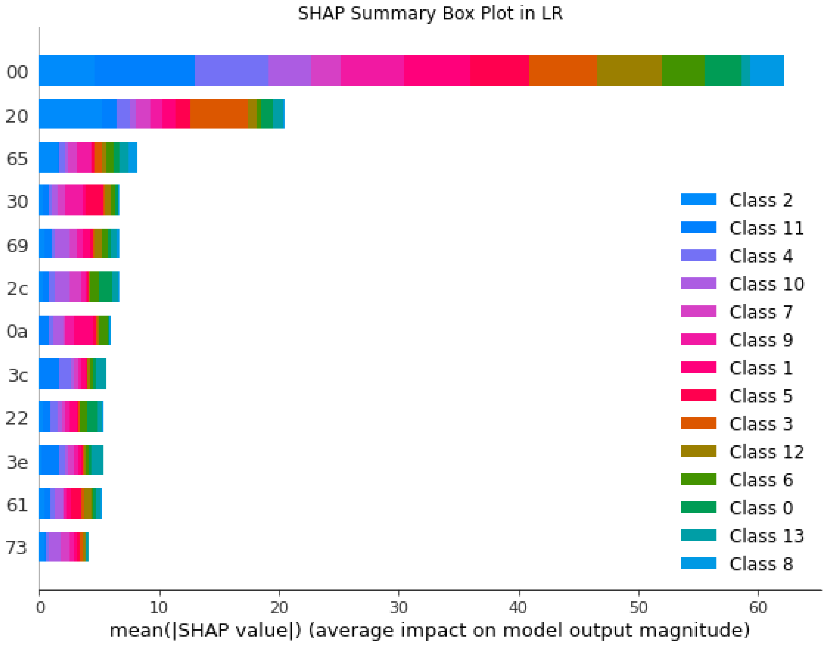
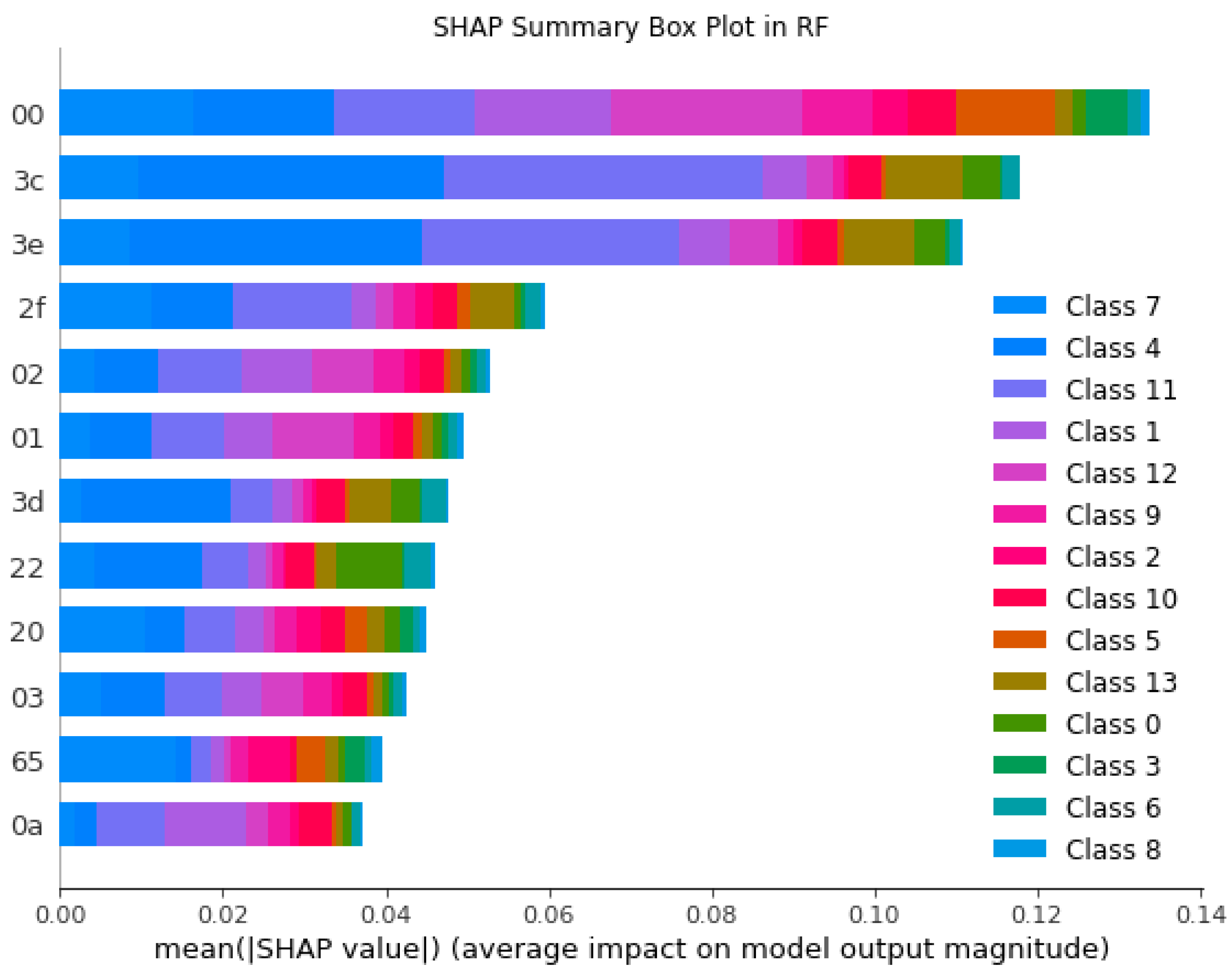
5.2.2. SHAP’s Global Interpretability

The SHAP global visualizations provide a comprehensive understanding of feature importance, revealing key patterns and associations within the dataset. First, we analyze the summary bar plots to obtain an overview of the feature importance for the models, then we use the beeswarm plots to obtain the actual direction and magnitude of the features with the individual classes.

The x-axis of the bar plot represents the average magnitude of the SHAP values for each feature across all instances. It is a measure of the average impact magnitude that each feature has on the model’s output. It depicts the influence of each feature on the model regardless of the direction of that influence. The y-axis lists the features and each row represents a feature. Each of the rows has a different bar length. The length of the bar in each row indicates the average impact of that particular feature on the model prediction. It signifies the influence of the feature. Hence, longer bars indicate a significant influence on the model’s prediction (i.e., whether it increases or decreases the prediction). The bytes are also arranged from top to bottom in order of importance. Additionally, the bars are color-coded with each class having a distinct color. The color shows which classes are most associated with the presence of each feature. For example, if the byte ‘00’ has a lot of blue in its bar, it means that this byte value is strongly associated with ‘Class 2’. Figure 12, Figure 13, Figure 14 and Figure 15 show the summary plot for LR, RF, SGD, and MLP models, respectively. They describe the average impact of features on the model output, which is averaged over all the samples in the dataset.

The LR model demonstrates a significant influence of features ‘00’, ‘20’, and ‘65’ across various classes, as indicated by the length of the bars. Notably, the impact of these features varies across classes, suggesting a nuanced relationship between feature values and class-specific predictions. Conversely, the RF model exhibits a more uniform distribution of feature impacts, with ‘00’, ‘3C’, ‘3E’, and ‘2F’ appearing as prominent across several classes. This uniformity could be indicative of the model’s reliance on an ensemble of decision trees which tend to give a more balanced consideration to the features. The SGD model, characterized by its linear nature and sensitivity to feature scaling, shows a different pattern of feature importance, with a few features such as ‘00’ and ‘20’ exerting disproportionately large effects on certain classes. This skew in feature impact distribution could reflect the SGD’s gradient descent optimization, which might lead to certain features being weighted more heavily in the linear decision boundary. The MLP model, harnessing the capability of deep learning to capture non-linear interactions, reveals a distinct pattern where features ‘3C’, ‘3E’, ‘0A’, and ‘00’ show a considerable impact on the predictions, alongside a broader spread of feature influences across various classes. This is consistent with the expectation that neural networks are adept at modeling complex, non-linear relationships in data.

Across all models, the presence of certain features as significant contributors to multiple classes suggests their pivotal role in the classification task, while the variation in their impact magnitude and direction underscores the diversity in modeling approaches. The differences in feature importance across the four models highlight the unique ways in which each algorithm processes and weighs the input data to arrive at a decision.

Although the bar plot shows a high-level overview of feature importance and impact direction, it cannot show or tell how each feature impacts the prediction based on the actual value of the feature. However, the beeswarm plot is meant for this insight. That is, the beeswarm plot can tell us if a high value or low value for a feature increases or decreases the likelihood of the model predicting a particular class.

For a beeswarm plot, the y-axis lists the features that influence the model’s predictions. Each dot on the plot represents the SHAP value for a feature for a single instance. Features are often ordered by the sum of SHAP value magnitudes across all samples, so the feature with the largest overall impact is usually at the top of the plot. The x-axis represents the SHAP value for each feature–instance pair. The SHAP values can be positive or negative. A positive SHAP value indicates that the presence of the feature pushes the model’s prediction higher (toward a particular class or a higher value). A negative SHAP value indicates that the feature contributes to a lower prediction value. The further from zero a dot is, the more impact that feature–instance pair has on the model’s output. The color of the dots often indicates the value of the feature for each instance, with one color representing higher values and another representing lower values. This color coding provides a visual cue as to how the value of a feature affects the prediction. The size of the dots can represent the density of points at that location, where larger dots indicate a higher overlap of instances with similar SHAP values for a feature. Figure 16, Figure 17, Figure 18 and Figure 19 show the beeswarm plots for LR, RF, SGD, and MLP, respectively.

Figure 16a illustrates how certain features increase or decrease the likelihood of the model predicting Class 0. For instance, the feature ‘00’ has high values (denoted in red) concentrated to the left. This implies that ‘00’ generally decreases the model’s output score for predicting Class 0. That is, higher values of ‘00’ are associated with a lower prediction for Class 0. Contrarily, the feature ‘2C’ with high values in the positive direction shows that higher values are influential in predicting Class 0. For Class 1, depicted in Figure 16b, feature ‘00’ has high values in the positive direction. This means that higher values of ‘00’ increase the likelihood of predicting Class 1.

In Figure 17a, representing Class 0, several features stand out due to their significant impact on the model’s prediction. Features ‘2C’ and ‘22’ show a movement of red dots to the right, suggesting that higher values of these features have a positive impact on the likelihood of an instance being classified as Class 0. Conversely, some features like ‘3E’ and ‘3D’ have a dispersion of blue dots toward the right, indicating that lower values of these features positively impact the prediction for Class 0.

Figure 17b, representing Class 1, displays a somewhat different pattern. Notably, features such as ‘0A’ and ‘02’ have a mixture of red and blue dots on both sides of the zero line, suggesting a more complex and variable relationship with Class 1 predictions. The spread of the dots indicates that the impact of these features on Class 1 predictions varies across different instances.

When comparing the beeswarm plots for Class 0 and Class 1, we observe that some features are influential for both classes, while others have a class-specific impact. This variability in feature contributions across classes underlines the RF model’s capacity to capture complex, non-linear interactions between features and classes. The presence of both positive and negative SHAP values for the same features across different classes indicates that the relationship between feature values and class predictions is not straightforward but rather depends on the interaction of the feature values within the context of each instance.

In Figure 18a (Class 0), we observe that several features such as ‘00’ and ‘30’ exhibit a strong negative relationship with the class prediction, as indicated by the red dots far to the left of the zero line. This suggests that higher values of these features are less likely to predict Class 0. On the other hand, feature ‘2C’ demonstrates a positive relationship, with red dots to the right, suggesting their higher values make Class 0 more likely.

Figure 18b (Class 1) reveals a contrasting pattern; for instance, ‘0A’ has a mix of positive and negative SHAP values, implying a complex and instance-specific relationship with the class prediction. Notably, the features ‘00’, ‘3C’, and ‘3E’ appear to have predominantly the same influence on both classes indicating that this feature may be critical for the SGD model.

In Figure 19a, for Class 0, we see a cluster of features (such as ‘2C’ and ‘22’) with negative SHAP values. This suggests that lower values of these features influence the model’s prediction away from Class 0. Conversely, there are fewer features with positive SHAP values, and they do not extend right, indicating that their influence in increasing the prediction toward Class 0 is less pronounced.

Figure 19b for Class 1 shows a different pattern. The features ‘0A’ and ‘00’ appear to have a mix of positive and negative SHAP values, suggesting that the impact of these features on the prediction for Class 1 can vary significantly between instances. Features that consistently show positive or negative SHAP values across both classes could be considered as having a stable influence on the model’s predictions, irrespective of the class. Features that show contrasting SHAP values between the two classes may be crucial in distinguishing between Class 0 and Class 1.

5.2.3. LIME’s Interpretability

Additionally, LIME’s local explanations delved into the granular details of individual predictions, highlighting the specific features that influenced each instance classification. Figure 20, Figure 21 and Figure 22 show the LIME report for the same test instance from the SHAP analysis. Figure 23 shows the report for another instance which is predicted as Class 10.

In the LIME plot, the x-axis represents the contribution or impact of that feature toward the predicted probability for each class. Specifically, the values indicate the magnitude and direction of the impact. A positive score indicates that increasing the value of the corresponding feature would contribute positively to the predicted probability of the class. A negative score indicates that increasing the value of the corresponding feature would contribute negatively to the predicted probability of the class. The y-axis shows the feature and its LIME threshold. The threshold indicates the point at which the feature is considered to be “small” or “large” in the local context. For example, if the original value of “65” for the instance is less than or equal to 52, it would be considered as “small” or “less than or equal to 83.79” in the local approximation. If the original value is greater than 83.79, it would be considered as “large” or “greater than 83.79” in the local approximation. These thresholds are determined by LIME to create a simplified, locally linear model that approximates the complex behavior of the underlying black-box model within a limited region around the instance of interest.

In Figure 20, the feature ‘74’ has a negative score of −0.87, suggesting that a lower ‘74’ value is associated with a higher probability of the predicted class. Conversely, feature ‘65’ has a positive score of 1.03, indicating that a higher ‘65’ value contributes positively to the probability of the instance. The features ‘22’, ‘65’, and ‘2C’ play a significant impact across the models for the chosen test instance for LR, RF, and SGD.

6. Conclusions

In this study, we used two XAI tools, SHAP and LIME, to analyze and interpret four machine learning models used in file fragment classification. These tools helped us understand how different features in the fragments affected the predictions made by these ML models.

SHAP analysis revealed diverse feature interactions across models through beeswarm and summary bar plots. SHAP values showed feature values’ relationship with class predictions, with some features impacting different classes positively or negatively. This variability highlights how models process data differently. SHAP beeswarm plots showcased feature impact distribution and magnitude. They highlighted the consistent importance of features like ‘00’ and ‘2C’ across models and their differential effects on classes. Summary bar plots further condensed the average feature effect, visualizing influential features and classes. SHAP waterfall plots added another dimension by detailing feature contributions to individual predictions. They allowed us to trace the prediction path and understand the additive impact of features. This granular view has been crucial for verifying prediction logic and enhancing model interpretability. LIME complemented SHAP by providing instance-level explanations, reinforcing key features, and offering a granular view. Combining insights from both SHAP and LIME provided a comprehensive understanding of the models’ behavior.

In summary, the combined use of SHAP and LIME interpretability tools has provided valuable insights into the decision-making process of machine learning models for file fragment classification. This analysis underscores the importance of Explainable Artificial Intelligence (XAI) in comprehensively understanding feature influences within such models. With these interpretability tools, we ensure high model accuracy as well as transparency and accountability.

In future work, we would integrate additional XAI techniques into machine learning models for file fragment classification to enhance interpretability. Furthermore, investigating the impact of different feature sets and model architectures on interpretability could lead to further advancements in this field. Ultimately, these efforts aim to improve model predictability and explainability, fostering trust and facilitating broader adoption of machine learning models in the domain of file fragment classification.

References

1. Jinad, R.; Islam, A.; Shashidhar, N. File Fragment Analysis Using Machine Learning. In Proceedings of the 2023 IEEE International Conference on Dependable, Autonomic and Secure Computing, International Conference on Pervasive Intelligence and Computing, International Conference on Cloud and Big Data Computing, International Conference on Cyber Science and Technology Congress (DASC/PiCom/CBDCom/CyberSciTech), Abu Dhabi, United Arab Emirates, 14–17 November 2023; pp. 956–962. [Google Scholar] [CrossRef]
2. Zhang, S.; Hu, C.; Wang, L.; Mihaljevic, M.J.; Xu, S.; Lan, T. A Malware Detection Approach Based on Deep Learning and Memory Forensics. Symmetry 2023, 15, 758. [Google Scholar] [CrossRef]
3. Sivalingam, K.M. Applications of Artificial Intelligence, Machine Learning and related Techniques for Computer Networking Systems. arXiv 2021, arXiv:2105.15103. [Google Scholar]
4. Goebel, R.; Chander, A.; Holzinger, K.; Lecue, F.; Akata, Z.; Stumpf, S.; Kieseberg, P.; Holzinger, A. Explainable AI: The new 42? In Proceedings of the Machine Learning and Knowledge Extraction: Second IFIP TC 5, TC 8/WG 8.4, 8.9, TC 12/WG 12.9 International Cross-Domain Conference, CD-MAKE 2018, Hamburg, Germany, 27–30 August 2018; Proceedings 2. Springer: Berlin/Heidelberg, Germany, 2018; pp. 295–303. [Google Scholar]
5. Arrieta, A.B.; Diaz-Rodriguez, N.; Del Ser, J.; Bennetot, A.; Tabik, S.; Barbado, A.; Garcia, S.; Gil-Lopez, S.; Molina, D.; Benjamins, R.; et al. Explainable Artificial Intelligence (XAI): Concepts, taxonomies, opportunities and challenges toward responsible AI. Inf. Fusion 2020, 58, 82–115. [Google Scholar] [CrossRef]
6. Beddiar, R.; Oussalah, M. Explainability in medical image captioning. In Explainable Deep Learning AI; Elsevier: Amsterdam, The Netherlands, 2023; pp. 239–261. [Google Scholar]
7. Gerlings, J.; Shollo, A.; Constantiou, I. Reviewing the need for explainable artificial intelligence (xAI). arXiv 2020, arXiv:2012.01007. [Google Scholar]
8. Gilpin, L.H.; Bau, D.; Yuan, B.Z.; Bajwa, A.; Specter, M.; Kagal, L. Explaining Explanations: An Overview of Interpretability of Machine Learning. In Proceedings of the 2018 IEEE 5th International Conference on Data Science and Advanced Analytics (DSAA), Turin, Italy, 1–3 October 2018; pp. 80–89. [Google Scholar] [CrossRef]
9. Lundberg, S.M.; Lee, S.I. A Unified Approach to Interpreting Model Predictions. In Advances in Neural Information Processing Systems 30; Guyon, I., Luxburg, U.V., Bengio, S., Wallach, H., Fergus, R., Vishwanathan, S., Garnett, R., Eds.; Curran Associates, Inc.: Glasgow, UK, 2017; pp. 4765–4774. [Google Scholar]
10. Ribeiro, M.T.; Singh, S.; Guestrin, C. “Why Should I Trust You?”: Explaining the Predictions of Any Classifier. In Proceedings of the 22nd ACM SIGKDD International Conference on Knowledge Discovery and Data Mining, (KDD ’16), San Francisco, CA, USA, 13–17 August 2016; pp. 1135–1144. [Google Scholar] [CrossRef]
11. Gohel, P.; Singh, P.; Mohanty, M. Explainable AI: Current status and future directions. arXiv 2021, arXiv:2107.07045. [Google Scholar]
12. Saeed, W.; Omlin, C. Explainable AI (XAI): A systematic meta-survey of current challenges and future opportunities. Knowl.-Based Syst. 2023, 263, 110273. [Google Scholar] [CrossRef]
13. Colley, A.; Väänänen, K.; Häkkilä, J. Tangible Explainable AI-an Initial Conceptual Framework. In Proceedings of the 21st International Conference on Mobile and Ubiquitous Multimedia, Lisbon, Portugal, 27–30 November 2022; pp. 22–27. [Google Scholar]
14. Pfeifer, B.; Krzyzinski, M.; Baniecki, H.; Saranti, A.; Holzinger, A.; Biecek, P. Explainable AI with counterfactual paths. arXiv 2023, arXiv:2307.07764. [Google Scholar]
15. Liao, Q.V.; Singh, M.; Zhang, Y.; Bellamy, R. Introduction to explainable AI. In Proceedings of the Extended Abstracts of the 2021 CHI Conference on Human Factors in Computing Systems, Yokohama, Japan, 8–13 May 2021; pp. 1–3. [Google Scholar]
16. Adadi, A.; Berrada, M. Peeking inside the black-box: A survey on explainable artificial intelligence (XAI). IEEE Access 2018, 6, 52138–52160. [Google Scholar] [CrossRef]
17. Farahani, F.V.; Fiok, K.; Lahijanian, B.; Karwowski, W.; Douglas, P.K. Explainable AI: A review of applications to neuroimaging data. Front. Neurosci. 2022, 16, 906290. [Google Scholar] [CrossRef]
18. Qian, J.; Li, H.; Wang, J.; He, L. Recent Advances in Explainable Artificial Intelligence for Magnetic Resonance Imaging. Diagnostics 2023, 13, 1571. [Google Scholar] [CrossRef]
19. Van der Velden, B.H.; Kuijf, H.J.; Gilhuijs, K.G.; Viergever, M.A. Explainable artificial intelligence (XAI) in deep learning-based medical image analysis. Med. Image Anal. 2022, 79, 102470. [Google Scholar] [CrossRef]
20. Ahmed, S.B.; Solis-Oba, R.; Ilie, L. Explainable-AI in Automated Medical Report Generation Using Chest X-ray Images. Appl. Sci. 2022, 12, 11750. [Google Scholar] [CrossRef]
21. Salahuddin, Z.; Woodruff, H.C.; Chatterjee, A.; Lambin, P. Transparency of deep neural networks for medical image analysis: A review of interpretability methods. Comput. Biol. Med. 2022, 140, 105111. [Google Scholar] [CrossRef]
22. Moraffah, R.; Karami, M.; Guo, R.; Raglin, A.; Liu, H. Causal interpretability for machine learning-problems, methods and evaluation. ACM SIGKDD Explor. Newsl. 2020, 22, 18–33. [Google Scholar] [CrossRef]
23. Rjoub, G.; Bentahar, J.; Wahab, O.A.; Mizouni, R.; Song, A.; Cohen, R.; Otrok, H.; Mourad, A. A Survey on Explainable Artificial Intelligence for Cybersecurity. IEEE Trans. Netw. Serv. Manag. 2023, 20, 5115–5140. [Google Scholar] [CrossRef]
24. Srivastava, G.; Jhaveri, R.; Bhattacharya, S.; Pandya, S.; Maddikunta, P.; Yenduri, G.; Hall, J.; Alazab, M.; Gadekallu, T. XAI for Cybersecurity: State of the Art, Challenges, Open Issues and Future Directions. arXiv 2022, arXiv:2206.03585. [Google Scholar]
25. Nadeem, A.; Vos, D.; Cao, C.; Pajola, L.; Dieck, S.; Baumgartner, R.; Verwer, S. Sok: Explainable machine learning for computer security applications. In Proceedings of the 2023 IEEE 8th European Symposium on Security and Privacy (EuroS&P), Delft, The Netherlands, 3–7 July 2023; pp. 221–240. [Google Scholar]
26. AL-Essa, M.; Andresini, G.; Appice, A.; Malerba, D. XAI to explore robustness of features in adversarial training for cybersecurity. In Proceedings of the International Symposium on Methodologies for Intelligent Systems, Cosenza, Italy, 3–5 October 2022; Springer: Berlin/Heidelberg, Germany, 2022; pp. 117–126. [Google Scholar]
27. Kuppa, A.; Le-Khac, N.A. Adversarial XAI methods in cybersecurity. IEEE Trans. Inf. Forensics Secur. 2021, 16, 4924–4938. [Google Scholar] [CrossRef]
28. Liu, H.; Zhong, C.; Alnusair, A.; Islam, S.R. FAIXID: A framework for enhancing AI explainability of intrusion detection results using data cleaning techniques. J. Netw. Syst. Manag. 2021, 29, 40. [Google Scholar] [CrossRef]
29. Suryotrisongko, H.; Musashi, Y.; Tsuneda, A.; Sugitani, K. Robust botnet DGA detection: Blending XAI and OSINT for cyber threat intelligence sharing. IEEE Access 2022, 10, 34613–34624. [Google Scholar] [CrossRef]
30. Kundu, P.P.; Truong-Huu, T.; Chen, L.; Zhou, L.; Teo, S.G. Detection and classification of botnet traffic using deep learning with model explanation. IEEE Trans. Dependable Secur. Comput. 2022; Early access. [Google Scholar]
31. Alani, M.M. BotStop: Packet-based efficient and explainable IoT botnet detection using machine learning. Comput. Commun. 2022, 193, 53–62. [Google Scholar] [CrossRef]
32. Barnard, P.; Marchetti, N.; DaSilva, L.A. Robust network intrusion detection through explainable artificial intelligence (XAI). IEEE Netw. Lett. 2022, 4, 167–171. [Google Scholar] [CrossRef]
33. Abou El Houda, Z.; Brik, B.; Khoukhi, L. “Why should i trust your ids?”: An explainable deep learning framework for intrusion detection systems in internet of things networks. IEEE Open J. Commun. Soc. 2022, 3, 1164–1176. [Google Scholar] [CrossRef]
34. Sivamohan, S.; Sri, S. KHO-XAI: Krill herd optimization and Explainable Artificial Intelligence framework for Network Intrusion Detection Systems in Industry 4.0. Res. Sq. 2022; preprint. [Google Scholar]
35. Mane, S.; Rao, D. Explaining network intrusion detection system using explainable AI framework. arXiv 2021, arXiv:2103.07110. [Google Scholar]
36. Wali, S.; Khan, I. Explainable AI and random forest based reliable intrusion detection system. TechRxiv, 2023; preprint. [Google Scholar]
37. Zebin, T.; Rezvy, S.; Luo, Y. An explainable AI-based intrusion detection system for DNS over HTTPS (DoH) attacks. IEEE Trans. Inf. Forensics Secur. 2022, 17, 2339–2349. [Google Scholar] [CrossRef]
38. Solanke, A.A. Explainable digital forensics AI: Toward mitigating distrust in AI-based digital forensics analysis using interpretable models. Forensic Sci. Int. Digit. Investig. 2022, 42, 301403. [Google Scholar] [CrossRef]
39. Gopinath, A.; Kumar, K.P.; Saleem, K.S.; John, J. Explainable IoT Forensics: Investigation on Digital Evidence. In Proceedings of the 2023 IEEE International Conference on Contemporary Computing and Communications (InC4), Bangalore, India, 21–22 April 2023; Volume 1, pp. 1–6. [Google Scholar]
40. Hall, S.W.; Sakzad, A.; Minagar, S. A Proof of Concept Implementation of Explainable Artificial Intelligence (XAI) in Digital Forensics. In Proceedings of the International Conference on Network and System Security, Denarau Island, Fiji, 9–12 December 2022; Springer: Berlin/Heidelberg, Germany, 2022; pp. 66–85. [Google Scholar]
41. Kelly, L.; Sachan, S.; Ni, L.; Almaghrabi, F.; Allmendinger, R.; Chen, Y. Explainable artificial intelligence for digital forensics: Opportunities, challenges and a drug testing case study. In Digital Forensic Science; IntechOpen: London, UK, 2020. [Google Scholar]
42. Lucic, A.; Srikumar, M.; Bhatt, U.; Xiang, A.; Taly, A.; Liao, Q.V.; de Rijke, M. A multistakeholder approach toward evaluating AI transparency mechanisms. arXiv 2021, arXiv:2103.14976. [Google Scholar]
43. Linardatos, P.; Papastefanopoulos, V.; Kotsiantis, S. Explainable AI: A review of machine learning interpretability methods. Entropy 2020, 23, 18. [Google Scholar] [CrossRef] [PubMed]
44. Doshi-Velez, F.; Kim, B. Toward a rigorous science of interpretable machine learning. arXiv 2017, arXiv:1702.08608. [Google Scholar]
45. Garfinkel, S.; Farrell, P.; Roussev, V.; Dinolt, G. Bringing science to digital forensics with standardized forensic corpora. Digit. Investig. 2009, 6, S2–S11. [Google Scholar] [CrossRef]
Figure 1. XAI Interpretability techniques.
Electronics 13 02438 g001
Figure 2. Limitations of XAI.
Electronics 13 02438 g002
Figure 3. Proposed methodology with ML Models and XAI Techniques.
Electronics 13 02438 g003
Figure 4. LR waterfall plots for Class 0 and Class 1.
Electronics 13 02438 g004
Figure 5. LR waterfall plots for Class 2 and Class 5.
Electronics 13 02438 g005
Figure 6. RF waterfall plots for Class 0 and Class 1.
Electronics 13 02438 g006
Figure 7. RF waterfall plots for Class 2 and Class 5.
Electronics 13 02438 g007
Figure 8. SGD waterfall plots for Class 0 and Class 1.
Electronics 13 02438 g008
Figure 9. SGD waterfall plots for Class 2 and Class 5.
Electronics 13 02438 g009
Figure 10. MLP waterfall plots for Class 0 and Class 1.
Electronics 13 02438 g010
Figure 11. MLP waterfall plots for Class 2 and Class 8.
Electronics 13 02438 g011
Figure 12. LR summary bar plot.
Electronics 13 02438 g012
Figure 13. RF summary bar plot.
Electronics 13 02438 g013
Figure 14. SGD summary bar plot.
Electronics 13 02438 g014
Figure 15. MLP summary bar plot.
Electronics 13 02438 g015
Figure 16. LR beeswarm plots. (a) Class 0; (b) Class 1.
Electronics 13 02438 g016
Figure 17. RF beeswarm plots. (a) Class 0; (b) Class 1.
Electronics 13 02438 g017
Figure 18. SGD beeswarm plots. (a) Class 0; (b) Class 1.
Electronics 13 02438 g018
Figure 19. MLP beeswarm plots. (a) Class 0; (b) Class 1.
Electronics 13 02438 g019
Figure 20. LR LIME plot.
Electronics 13 02438 g020
Figure 21. RF LIME plot.
Electronics 13 02438 g021
Figure 22. SGD LIME plot.
Electronics 13 02438 g022
Figure 23. MLP LIME plot.
Electronics 13 02438 g023