Mission-Conditioned Path Planning with Transformer Variational Autoencoder

Abstract

This paper introduces a novel deep learning framework for robotic path planning that addresses two primary challenges: integrating mission specifications defined through Linear Temporal Logic (LTL) and enhancing trajectory quality via cost function integration within the configuration space. Our approach utilizes a Conditional Variational Autoencoder (CVAE) to efficiently encode optimal trajectory distributions, which are subsequently processed by a Transformer network. This network leverages mission-specific information from LTL formulas to generate control sequences, ensuring adherence to LTL specifications and the generation of near-optimal trajectories. Additionally, our framework incorporates an anchor control set—a curated collection of plausible control values. At each timestep, the proposed method selects and refines a control from this set, enabling precise adjustments to achieve desired outcomes. Comparative analysis and rigorous simulation testing demonstrate that our method outperforms both traditional sampling-based and other deep-learning-based path-planning techniques in terms of computational efficiency, trajectory optimality, and mission success rates.

1. Introduction

Path planning is a cornerstone of robotics, evolving from simple two-dimensional navigation to addressing more complex systems such as robot manipulators [1,2,3] and challenging scenarios [4,5,6]. This evolution underscores the necessity for sophisticated path-planning algorithms capable of navigating both the physical aspects of environments and the intricate requirements of diverse tasks.

Translating mission specifications, often articulated in human language, into computational models presents a significant challenge in path planning. Formal methods such as Linear Temporal Logic (LTL), Computation Tree Logic (CTL), and $\mu$-calculus are pivotal in this area. LTL, in particular, is favored for its flexibility and expressive power in defining complex missions [7,8,9], offering a structured yet adaptable framework for encoding mission objectives.

Additionally, the quest for trajectories that balance cost-effectiveness with computational efficiency is critical. For instance, in environments with variable communication strengths, it is crucial to find low-cost paths that minimize exposure to areas with poor connectivity. Traditional methods like Rapidly Exploring Random Tree Star (${\mathrm{RRT}}^{*}$) [10] are effective but can be computationally demanding, especially under numerous constraints.

The integration of deep learning into path planning offers a promising alternative, excelling in deriving optimal paths directly from data, thus mitigating the computational drawbacks of conventional methods. These techniques have broadened their utility across various domains, enhancing control strategies for robot manipulators [1] and addressing complex challenges in autonomous vehicle navigation [11,12]. The versatility and computational efficiency of deep learning approaches continue to propel advancements in the field of robotics.

This paper introduces a novel deep learning framework for robotic path planning that seamlessly integrates Linear Temporal Logic (LTL) formulas for mission specification with advanced trajectory optimization techniques. Our model employs a Conditional Variational Autoencoder (CVAE) and a Transformer network to innovatively generate control sequences that adhere to LTL specifications while optimizing cost efficiency. This integration marks a significant advancement in the fusion of deep learning with formal methods for path planning.

Key contributions of our approach include:

• Application of the Transformer Network:We utilize the Transformer network to interpret LTL formulas and generate control sequences [13]. This allows for the effective handling of complex mission specifications.
• Conditional Variational Autoencoder (CVAE): The CVAE is employed to navigate complex trajectory manifolds [14], providing the capability to generate diverse and feasible paths that meet the mission requirements.
• Anchor Control Set: Our framework includes an anchor control set—a curated collection of plausible control values. At each timestep, the method selects and finely adjusts a control from this set, ensuring precise trajectory modifications to achieve desired objectives.
• Incorporation of a Gaussian Mixture Model (GMM): The integration of a GMM to refine outputs enhances our framework’s capacity to handle uncertainties, thereby improving both the precision and reliability of path planning under LTL constraints.

These contributions collectively advance efficient robotic path planning by providing near-optimal solutions that satisfy given LTL formulas.

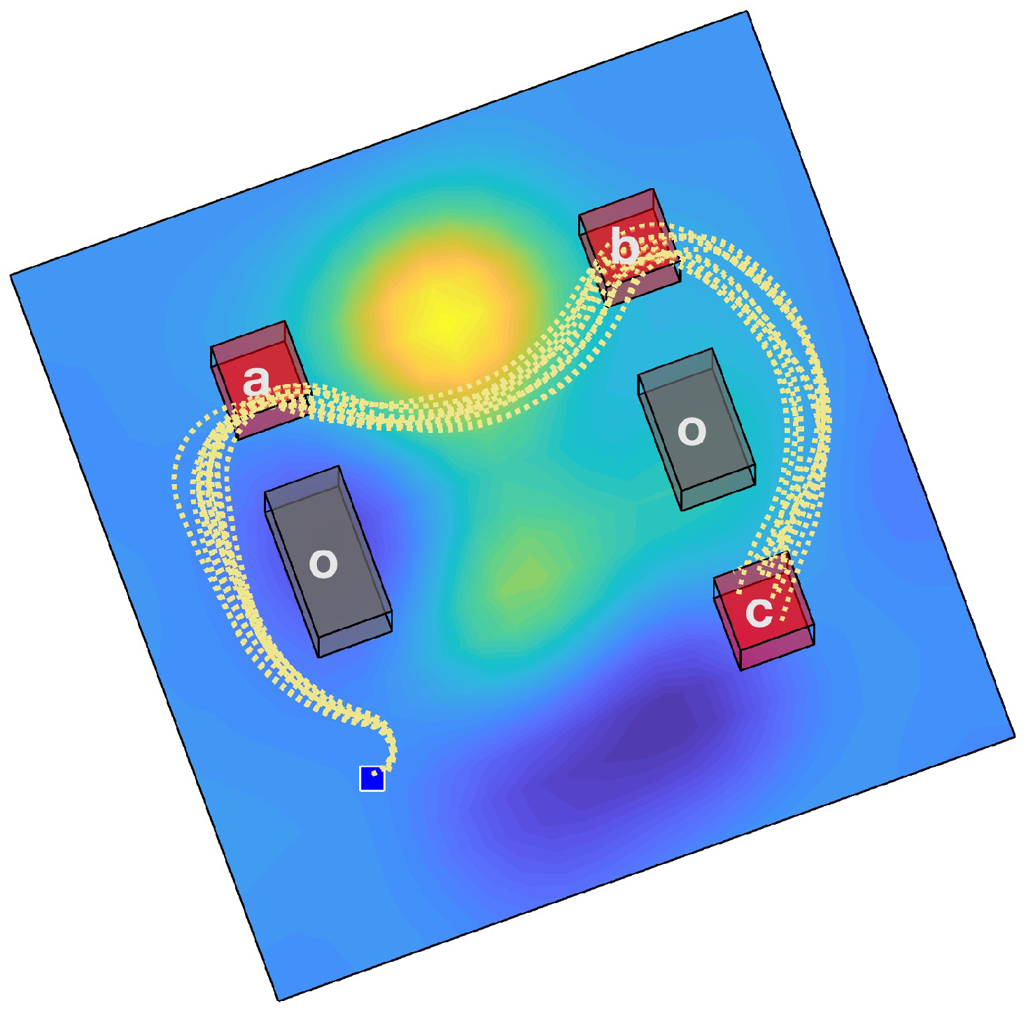
As illustrated in Figure 1, our method synthesizes a control sequence distribution, enhanced by a GMM, for a given test scenario that adheres to the LTL formula $\varphi =◊(a\wedge ◊(b\wedge (◊c)\left)\right)$. This formula requires sequentially visiting regions a, b, and c. The figure displays trajectories sampled from the output control sequence distribution generated by the proposed approach. It is notable that these trajectories navigate through low-cost areas (depicted in blue) while avoiding obstacles and fulfilling the specified LTL requirements.

Our contributions establish new benchmarks for cost efficiency and computational performance in robotic path planning. The effectiveness and superiority of our model compared to existing deep-learning-based strategies are demonstrated through rigorous comparative simulations, showcasing its potential to significantly influence the field.

2. Related Work

Path planning is a foundational element of robotics, requiring a balance between low-cost trajectories, complex dynamics, and precise mission specifications. The literature offers a diverse range of strategies addressing these challenges with varying degrees of success.

Finite Deterministic Systems: Research in finite deterministic systems has explored optimal controls with varied cost functions, such as minimax for bottleneck path problems [15] and weighted averages for cyclic paths [16]. However, these approaches often struggle in continuous path-planning scenarios due to limitations in integrating robot dynamics and the necessity for high-resolution discretization.

Sampling-based Motion Planning: Sampling-based methods, such as Rapidly Exploring Random Tree (RRT) [17], have addressed the integration of temporal logic and complex dynamics. The Rapidly Exploring Random Graph (RRG) [18] and Rapidly Exploring Random Tree Star (${\mathrm{RRT}}^{*}$) [19] demonstrate utility in optimizing motion planning but face scalability and efficiency challenges as complexity increases.

Multi-layered Frameworks: Multi-layered frameworks that blend discrete abstractions with automata for co-safe LTL formulas [20,21,22] guide trajectory formation using sampling-based methods. Despite advancements, these approaches often rely heavily on geometric decomposition, which limits their computational efficiency.

Optimization Methods: Optimization techniques, especially those utilizing mixed-integer programming, aim to achieve optimal paths under LTL constraints [23,24]. Although effective, these methods encounter scalability issues when dealing with complex LTL formulas and a growing number of obstacles. The cross-entropy-based planning algorithm [25] enhances efficiency but also struggles with extensive LTL formulas.

Learning from Demonstration (LfD): LfD has increasingly integrated temporal logic to enhance autonomous behaviors, employing strategies such as Monte Carlo Tree Search (MCTS) adjusted with STL robustness values to enhance constraint satisfaction [26]. This integration illustrates LfD’s potential in continuous control scenarios [27], with significant developments in blending formal task specifications within LfD skills using STL and black-box optimization for skill adaptation [28].

Trajectory Forecasting: Recent advances in trajectory forecasting have utilized deep learning to predict future movements based on past data, aligning closely with LfD principles. This research employs models such as Gaussian Mixture Models (GMMs) and Variational Autoencoders with Transformer architectures to produce action-aware predictions [29,30]. These approaches push the envelope toward models that seamlessly integrate global intentions with local movement strategies for improved adaptability and accuracy [31].

3. Preliminaries

This section introduces the foundational concepts and notations critical for understanding our approach to path planning under LTL specifications. Establishing a clear framework is essential for a comprehensive presentation of the system model, dynamics, and temporal logic that articulates the desired path properties. We will outline the mathematical formulations that underpin our system’s model, explain the dynamics governing the system, and detail the principles of LTL that are crucial for defining and evaluating trajectory objectives. This groundwork is vital for understanding the complexities of autonomous systems and their operational criteria, preparing the ground for a detailed exploration of our proposed method.

3.1. System Model

To establish a foundation for our system model, we first introduce essential notations:

• $\mathcal{X}\subset {\mathbb{R}}^n$               : The system’s state space.
• ${\mathcal{X}}_{obs}\subset {\mathbb{R}}^n$           : Space occupied by obstacles.
• ${\mathcal{X}}_{free}=\mathcal{X}\setminus {\mathcal{X}}_{obs}$ : Free space not occupied by obstacles.
• $\mathcal{U}\subset {\mathbb{R}}^m$              : Set of feasible controls.
• $\mathcal{W}\subset {\mathbb{R}}^{n_w}$           : Workspace in which the system operates.
• $h:\mathcal{X}\to \mathcal{W}$          : Mapping function from the state space to the workspace.

The system’s dynamics are described by the following equation:

$${\dot{\mathrm{x}}}_t=f({\mathrm{x}}_t,{\mathrm{u}}_t),$$

(1)

where ${\mathrm{x}}_t\in {\mathcal{X}}_{free}$ represents the state of the system, ${\mathrm{u}}_t\in \mathcal{U}$ denotes the control input, and f is a continuously differentiable function.

Given a control signal $\mathbf{u}$ over a time interval $[0,T]$, the resulting trajectory $\mathbf{x}({\mathrm{x}}_0,\mathbf{u})$ starts from the initial state ${\mathrm{x}}_0$. The state of the system along this trajectory at any given time $t\in [0,T]$ is denoted by $\mathbf{x}({\mathrm{x}}_0,\mathbf{u},t)$.

For discrete analysis, the trajectory $\mathbf{x}({\mathrm{x}}_0,\mathbf{u})$ is sampled at time increments $\Delta t\in {\mathbb{R}}^{+}$, expressed as:

$${\mathbf{x}}_{\Delta t}({\mathrm{x}}_0,\mathbf{u})={\left\{\mathbf{x}({\mathrm{x}}_0,\mathbf{u},i\Delta t)\right\}}_{i=0}^{i_f},$$

(2)

where $i_f\in \mathbb{N}$ is the final time step, chosen based on the trajectory analysis requirements. This sampling ensures that the discrete representation accurately captures the essential dynamics of the trajectory over the analysis period, balancing computational efficiency with simulation accuracy.

3.2. Linear Temporal Logic (LTL)

LTL is a formalism used to express properties over linear time [32]. It utilizes atomic propositions (APs), Boolean operators, and temporal operators. An atomic proposition is a simple statement that is either true or false. Essential LTL operators include ◯ (next), U (until), □ (always), ◊ (eventually), and ⇒ (implication). The structure of LTL formulas adheres to a grammar outlined in [33].

In our framework, $\Pi =\{{\pi }_0,{\pi }_1,\dots ,{\pi }_N\}$ denotes the set of all atomic propositions. An LTL trace, represented as $\sigma$, is a sequence of atomic propositions. LTL typically deals with infinite traces, with ${\Sigma }^{\omega }$ representing all possible infinite traces originating from $\Sigma =2^{\Pi }$. A trace $\sigma$ satisfies a formula $\varphi$ if it is expressed as $\sigma \vDash \varphi$.

For this study, we focus on finite-time path planning using syntactically co-safe LTL (sc-LTL) formulas [34], which are particularly suited for finite scenarios. A sc-LTL formula $\varphi$ ensures that any infinite trace satisfying $\varphi$ also has a finite prefix that satisfies $\varphi$. All temporal logic formulas discussed in this paper adhere to the sc-LTL format.

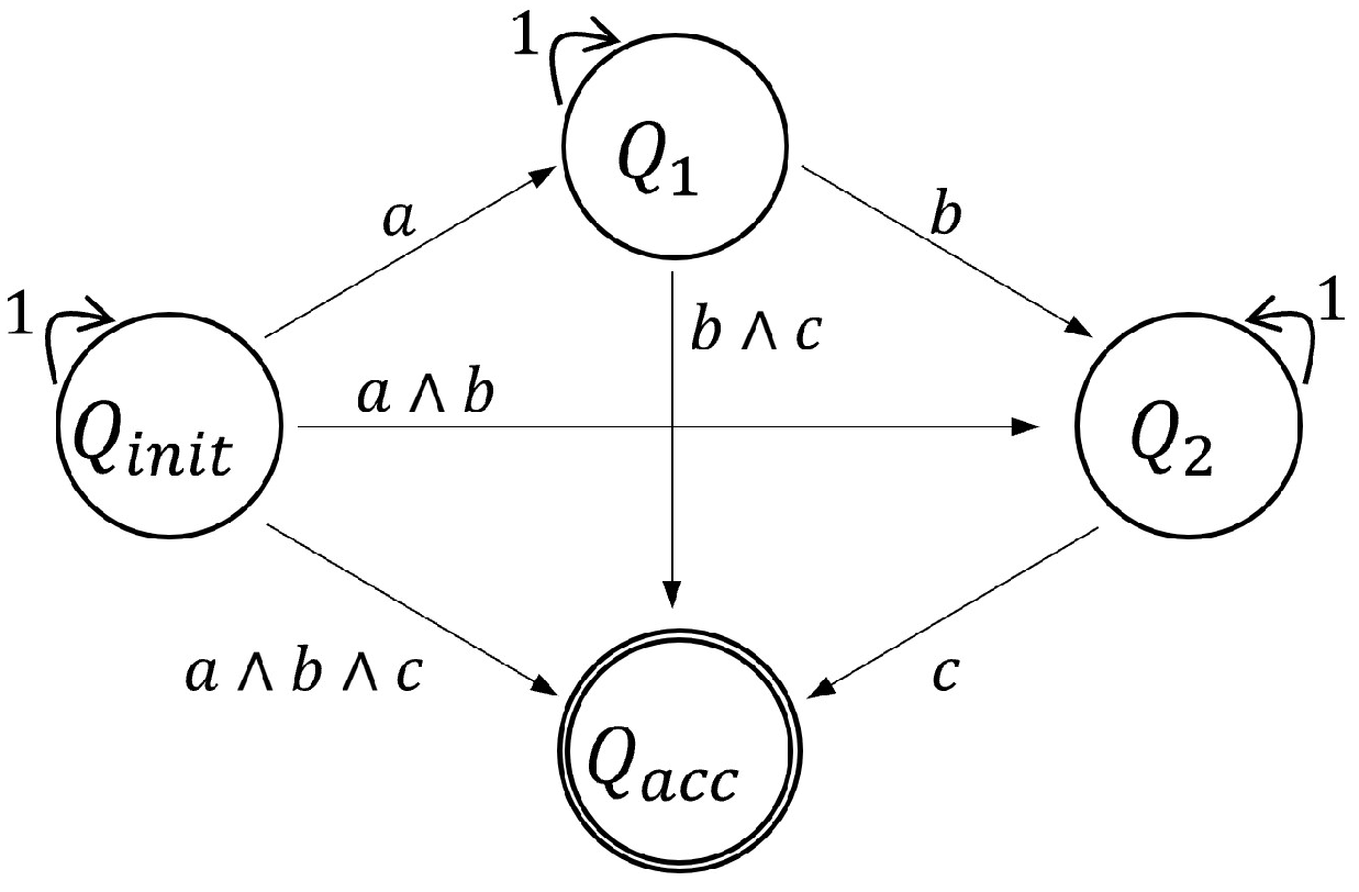
3.2.1. Automaton Representation

Given a set of atomic propositions $\Pi$ and a syntactically co-safe LTL formula $\varphi$, a nondeterministic finite automaton (NFA) can be constructed [35]. For instance, for the formula $\varphi =◊(a\wedge ◊(b\wedge ◊\left(c\right)\left)\right)$, an example of the resulting NFA is depicted in Figure 2. This NFA can be converted into a deterministic finite automaton (DFA), which is more suitable for computational processes. A DFA is described by the tuple ${\mathcal{A}}_{\varphi }=(Q,\Sigma ,\delta ,q_{init},Q_{acc})$, where:

• Q                           : Set of states
• $\Sigma =2^{\Pi }$                 : Alphabet, where each letter is a set of propositions
• $\delta :Q\times \Sigma \to Q$     : Transition function
• $q_{init}\subseteq Q$               : Initial state(s)
• $Q_{acc}\subseteq Q$              : Accepting states

A trace $\sigma$ from a DFA is accepted if, at any point, it leads to one of the accepting states (i.e., ${\sigma }_i\cap Q_{acc}\ne \varnothing$). Thus, a trace satisfies the sc-LTL formula $\varphi$ (denoted as $\sigma \vDash \varphi$) if it is accepted by the DFA ${\mathcal{A}}_{\varphi }$.

3.2.2. LTL Semantics over Trajectories

In this work, we define regions of interest within the workspace, $\mathcal{W}$, as $P=\{P_1,...,P_n\}$. These regions of interest are specified by the user. Each atomic proposition, ${\pi }_j$, from the set $\Pi$, corresponds to a specific region of interest, $P_j$. We employ a labeling function, $L:\mathcal{W}\to 2^{\Pi }$, to map each point in the workspace to a set of atomic propositions that are valid at that location. For any ${\pi }_i\in \Pi$, the negation $\neg {\pi }_i$ holds true for all points $\{w\in \mathcal{W}|{\pi }_i\notin L\left(w\right)\}$. Notably, ${\pi }_0$ remains true in all areas of the workspace except for the defined regions of interest and obstacles.

For a discretized trajectory, represented as ${\mathbf{x}}_{\Delta t}(x_0,\mathbf{u})={\mathrm{x}}_0,{\mathrm{x}}_1,...,{\mathrm{x}}_m$, which originates from ${\mathrm{x}}_0$ and follows the control inputs $\mathbf{u}$ at each time step $\Delta t$, the trajectory trace can be defined as follows [20]:

$$trace\left({\mathbf{x}}_{\Delta t}({\mathrm{x}}_0,\mathbf{u})\right)=L\left(h\left({\mathrm{x}}_0\right)\right),L\left(h\left({\mathrm{x}}_1\right)\right),...,L\left(h\left({\mathrm{x}}_m\right)\right).$$

(3)

This trace captures the sequence of atomic propositions valid at each point along the trajectory, reflecting the dynamic interaction with the workspace.

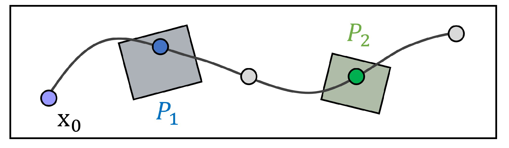
Figure 3 illustrates an example of a trajectory and its associated trace. This visual representation aids in understanding how the discrete segments of a trajectory map to their corresponding traces. For a given trajectory trace $trace\left({\mathbf{x}}_{\Delta t}({\mathrm{x}}_0,\mathbf{u})\right)={\tau }_0,{\tau }_1,...,{\tau }_m$, we define the automaton state sequence ${\mathcal{A}}_{\varphi }\left(trace\left({\mathbf{x}}_{\Delta t}({\mathrm{x}}_0,\mathbf{u})\right)\right)=q_0,q_1,...,q_m$ with each $q_k$ specified as:

$$q_k=\left\{\begin{array}{cc}\delta (q_{init},{\tau }_0)\hfill & \mathrm{if}k=0\hfill \\ \delta (q_{k-1},{\tau }_k)\hfill & \mathrm{if}k>0\hfill \end{array}\right..$$

(4)

A trajectory ${\mathbf{x}}_{\Delta t}({\mathrm{x}}_0,\mathbf{u})$ complies with the LTL formula $\varphi$, denoted by $\mathbf{x}({\mathrm{x}}_0,\mathbf{u}){\vDash }_{\Delta t}\varphi$, if the automaton sequence reaches a subset of the accepting states $Q_{acc}$.

4. Proposed Method

Our approach primarily focuses on optimizing the accumulated cost $J({\mathrm{x}}_0,\mathbf{u})$, which is the line integral of a cost function c over a trajectory, mathematically expressed as:

$$J({\mathrm{x}}_0,\mathbf{u})=\frac{1}{T}{\int }_0^{T}c\left(\mathbf{x}({\mathrm{x}}_0,\mathbf{u},t)\right)dt,$$

(5)

where $c:\mathcal{X}\to {\mathbb{R}}^{+}$ is a bounded and continuous cost function, $\mathbf{u}$ represents the control signal from $t=0$ to $t=T$, and ${\mathrm{x}}_0$ is the initial state. Mission tasks are defined using a syntactically co-safe LTL formula, with each atomic proposition associated with a specific region of interest.

This paper introduces a novel deep learning framework for robotic path planning that significantly advances the synthesis of near-optimal control sequences. Our method is designed to meet specific mission requirements, adhere to system dynamics (as defined in Equation (1)), and optimize cost efficiency (as outlined in Equation (5)).

At the core of our innovative approach is the integration of a Conditional Variational Autoencoder (CVAE) with Transformer networks, creating an end-to-end solution that represents a significant leap forward in path-planning research. The CVAE plays a crucial role in learning the distribution within the latent space of optimal control sequences, enabling the generation of sequences that satisfy LTL constraints while minimizing costs.

Our methodology leverages convolutional neural networks (CNNs) to transform environmental inputs—such as cost maps, regions of interest, and obstacle configurations—into an image-like format, thus optimizing the processing of spatial information.

A distinctive feature of our research is the introduction of an anchor control set. Instead of directly generating a control sequence, our method selects an appropriate control from the anchor control set at each timestep. This selection and subsequent refinement are facilitated by a Gaussian Mixture Model (GMM), which effectively accounts for environmental uncertainties. This approach enables more precise control predictions and enhances the system’s robustness against dynamic and unpredictable conditions.

The process begins with the Transformer’s decoder generating an initial anchor control value, which is then refined by the GMM to incorporate minor uncertainties. This integration, bolstered by learning from the latent distribution, significantly improves the precision and reliability of control sequence predictions. Our structured approach innovatively addresses uncertainties, thereby enhancing the robustness of our path-planning framework.

In summary, the proposed method offers several key advantages:

• End-to-end approach: By employing a Transformer network to encode LTL formulas, our method eliminates the need for the discretization processes and graph representations typically required in previous studies. This streamlined approach simplifies the encoding and handling of complex specifications directly within the network architecture.
• Step-by-step uncertainty consideration: Our approach meticulously addresses uncertainties within the path-planning process. The latent space is designed to account for major uncertainties, while the selection of controls from the anchor control set and their subsequent refinement through the GMM framework effectively manage minor uncertainties, enhancing the robustness and reliability of the trajectory planning.

Subsequent sections will delve deeper into our methodology, particularly focusing on the innovative implementation of anchor controls within the GMM framework and its profound implications. Through this detailed exploration, we aim to provide a clear understanding of the significant advancements our strategy introduces to the field of path planning.

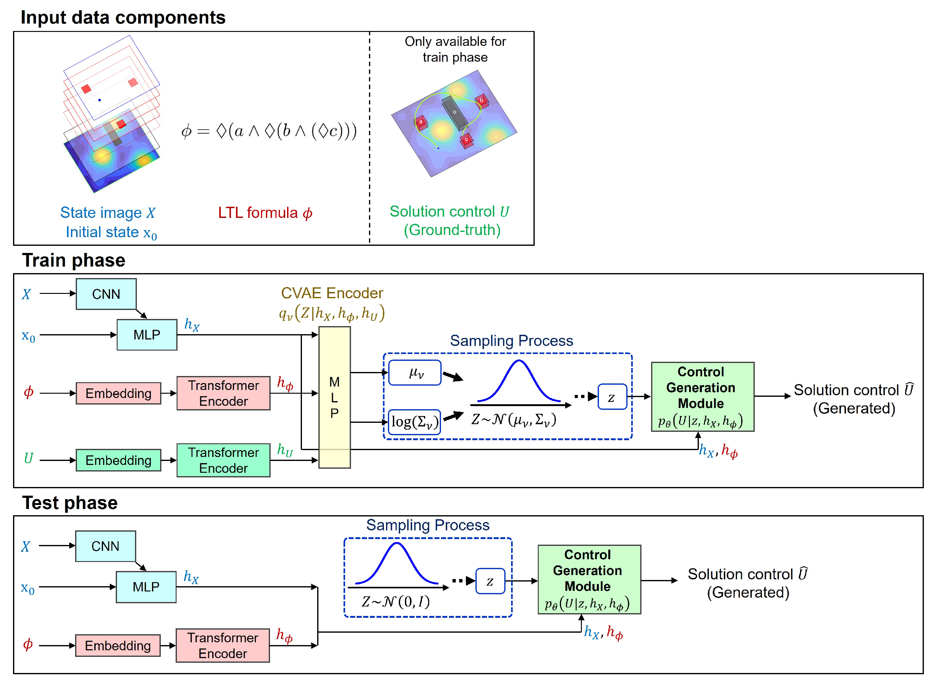
4.1. Data Components

This section outlines the input configurations employed in our deep learning framework, designed to facilitate the interpretation of LTL formulas. To simplify the association of LTL formulas with spatial regions, regions of interest within the operational environment are denoted alphabetically, starting with a.

Our framework utilizes two primary data components: the state image X and the solution control sequence U. The state image X consists of multiple layers, each representing different environmental features in a format readily processed by the neural network. As illustrated in Figure 4, these layers include the costmap, obstacles, regions of interest, and the initial position, with each layer stacked to provide a comprehensive environmental context.

The generation of control sequences is guided by methodologies from our prior research [36], which align with our system dynamics as defined in Equation (1) and the specifications of co-safe temporal logic. Specifically, the adopted approach focuses on identifying low-cost trajectories that comply with given co-safe temporal logic specifications, with LTL semantics evaluated against the trajectories to ensure adherence to necessary specifications.

Our data generation strategy is specifically tailored to accommodate environmental constraints and LTL objectives relevant to our study. This strategy is depicted in Figure 5, illustrating how environmental parameters and LTL formulas are transformed into output control sequences. When the length of generated sequences falls short of the maximum designated length, dummy control values are utilized as placeholders to maintain uniform sequence length, aiding in standardizing the training process across different scenarios.

4.2. Anchor Control Set

In our proposed model, we utilize an anchor control set $\mathbf{A}={\left\{{\mathbf{a}}^k\right\}}_{k=1}^K$, consisting of a predefined, fixed set of control sequences. Each anchor control, ${\mathbf{a}}^k$, is a sequence of control inputs $[{\mathrm{u}}_0^k,{\mathrm{u}}_1^k,\dots ,{\mathrm{u}}_{H_A-1}^k]$ that spans a designated time horizon $H_A$. It is important to note that this time horizon $H_A$ is not necessarily equivalent to the time horizon of the final solution’s control sequence.

The use of longer sequences for each anchor control, rather than single timestep controls, is motivated by the difficulty of capturing significant behavioral trends with overly granular, single-step data. In the control generation stage of our network, which will be elaborated on in subsequent sections, controls are selected in bundles of $H_A$ rather than individually per timestep. This approach simplifies the decoder’s prediction tasks compared to methods that operate on a per-timestep basis, thereby enhancing both the efficiency and efficacy of our model.

To construct the anchor control set, we derived it from a dataset using the k-means clustering algorithm. The distance between two anchor controls, necessary for the clustering process, is calculated as follows [29]:

$$d({\mathbf{a}}^i,{\mathbf{a}}^j)=\sum _{t=0}^{H_A}{\parallel {\mathrm{u}}_t^i-{\mathrm{u}}_t^j\parallel }^2.$$

(6)

This metric ensures that the controls within our set are optimally spaced to effectively cover diverse potential scenarios.

4.3. Proposed Architecture

The architecture of our proposed deep learning network is depicted in Figure 6. This comprehensive end-to-end system processes inputs from the environmental image and LTL formula to the final generation of the control sequence.

• Data components (1st row): The input layer consists of the multi-channeled state image X, the initial state $x_0$, the LTL formula $\varphi$, and the solution control sequence U. These components establish the context and objectives for path planning.
• Training phase (2nd row): During training, the network utilizes the solution control sequence U from the dataset to train the Conditional Variational Autoencoder (CVAE). This enables the network to effectively learn the latent distribution, facilitating accurate prediction of the control sequence $\widehat{U}$ that adheres to the LTL specifications.
• Testing phase (3rd row): In the testing phase, the architecture demonstrates how latent samples are converted into predicted control sequences, validating the trained model’s efficacy in real-world scenarios.

This network not only streamlines the transition from input to output but also ensures that all elements, from environmental conditions to control strategies, are integrated within a unified framework. By detailing each phase of the network, we provide a clear pathway from data ingestion to practical application, highlighting the network’s capacity to adapt and respond to complex path-planning demands.

In the encoding stage, the network processes the input data using specialized components. A CNN encodes the state image, while Transformer encoders [13] handle the encoding of control sequences and LTL formulas. The LTL formulas are encoded by transforming each character into an embedded representation using a predefined set of alphabet and operator symbols. The resulting encoded outputs—$h_X$ for the state image X and initial state $x_0$, $h_{\varphi }$ for the LTL formula $\varphi$, and $h_U$ for the solution control sequence U—are then integrated to facilitate the learning process.

A key feature of our network is the implementation of a CVAE, chosen for its efficacy in handling high-dimensional spaces and versatility with various input configurations. The CVAE is instrumental in generating output control sequences by exploring the latent space. During training, it learns a probability distribution representing potential control sequences, conditioned on the encoded state image $h_X$ and LTL formula features $h_{\varphi }$.

Our CVAE model includes three crucial parameterized functions:

• The recognition model $q_{\nu }\left(Z\right|h_X,h_{\varphi },h_U)$ approximates the distribution of the latent variable Z based on the input features and the control sequence. It is modeled as a Gaussian distribution, $\mathcal{N}({\mu }_{\nu }(h_X,h_{\varphi },h_U),{\Sigma }_{\nu }(h_X,h_{\varphi },h_U))$, where ${\mu }_{\nu }$ and ${\Sigma }_{\nu }$ represent the mean and covariance determined by the network.
• The prior model $p_{\theta }\left(Z\right|h_X,h_{\varphi })$ assumes a standard Gaussian distribution, $\mathcal{N}(0,I)$, simplifying the structure of the latent space.
• The generation model $p_{\theta }\left(U\right|z,h_X,h_{\varphi })$ calculates the likelihood of each control sequence element $u_i$ based on the latent sample z and the encoded inputs, computed as the product of conditional probabilities over the sequence’s length $N_A\times H_A$. This model is implemented in the Control Generation Module depicted in Figure 7.

A sample z drawn from the recognition model is fed into the decoder, which then generates the predicted control sequence. The length of this control sequence is $N_A\times H_A$, reflecting the selection of $N_A$ anchor controls, each with a time length of $H_A$.

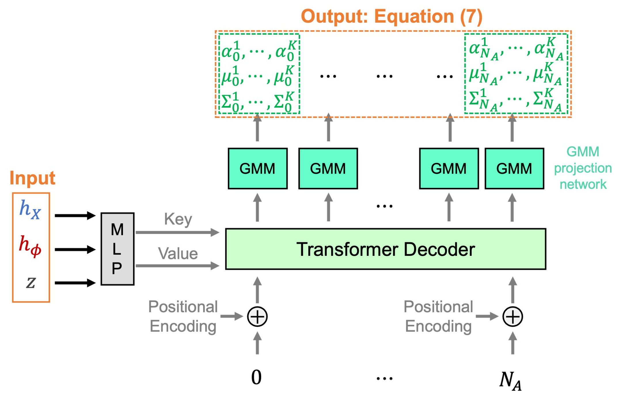
4.4. Control Generation Module

The architecture of our proposed control generation module is depicted in Figure 7. This module efficiently synthesizes the entire control sequence distribution from the latent sample z and encoded information $h_X,h_{\varphi }$ in a single step, utilizing a non-autoregressive model to enhance efficiency and coherence. The GMM projection networks share parameters across all calculations, ensuring consistency.

In this model, a Transformer decoder utilizes sinusoidal positional encodings to integrate time information as the query, while the latent vector, combined with the encoded state image and LTL formula features, acts as the key and value. This configuration, coupled with a GMM mixture module, enables the Transformer decoder to generate the output control sequence distribution as defined by the following equation:

$$p_{\theta }\left(U\right|z,h_X,h_{\varphi })=\prod _{t=0}^{N_A}\sum _{k=1}^K{\alpha }_t^k\mathcal{N}\left({\tilde{u}}_t|{\mathbf{a}}^k+{\mu }_t^k,{\Sigma }_t^k\right).$$

(7)

In this formulation:

• ${\alpha }_t^k$, ${\mu }_t^k$, and ${\Sigma }_t^k$ are the mixture coefficients, means, and covariances of the GMM, respectively, produced by the GMM projection network.
• ${\mathbf{a}}^k$ represents the anchor control from the set A.
• K is the number of mixture components, equal to the number of anchor controls, demonstrating the model’s capability to represent complex distributions of control sequences.
• Each ${\tilde{u}}_t$ spans the time horizon $H_A$.

This approach uses the GMM to integrate the latent variable z, historical state image data $h_X$, and LTL formula features $h_{\varphi }$, creating a probabilistic space where potential control sequences are distributed around the anchor control ${\mathbf{a}}^k$. This serves as a central reference point, enabling the identification of feasible control sequences within the operational domain. Unlike static models, ${\mathbf{a}}^k$ and the GMM adapt predictions to varying conditions and uncertainties inherent in dynamic environments, enhancing the model’s flexibility.

To maintain focus on the model’s predictive capability and avoid unnecessary complexity, we present the GMM parameters directly without delving into the detailed functional dependencies on $\theta$. This straightforward presentation underscores the model’s utility in forecasting control sequences that are both feasible and optimized according to the computed probability distributions.

4.5. Loss Function for Training Phase

The training of our CVAE is governed by the Evidence Lower Bound (ELBO) loss function, which is initially formulated as:

$${\mathbb{E}}_{q_{\nu }\left(Z\right|h_X,h_{\varphi },h_U)}[log{p}_{\theta }\left(U\right|z,h_X,h_{\varphi })]-{\mathcal{D}}_{KL}\left(q_{\nu }\left(z\right|h_X,h_{\varphi },h_U)\left|\right|p_{\theta }\left(z\right|h_X,h_{\varphi })\right).$$

(8)

To better suit our application’s specific requirements, we adapt the ELBO function and define the loss function as follows:

$$-{\sum }_{t=0}^{N_A}log\left(p_{\theta }\left({\tilde{u}}_t\right|z,h_X,h_{\varphi })\right)+\lambda ·{\mathcal{D}}_{KL}\left(\mathcal{N}\left({\mu }_{\nu }(h_X,h_{\varphi },h_U),{\Sigma }_{\nu }(h_X,h_{\varphi },h_U)\right)\left|\right|\mathcal{N}(0,I)\right),$$

(9)

where ${\tilde{u}}_t$ represents an element of the control sequence U, $N_A$ is the number of anchor controls, and $\lambda$ is a scaling factor used to balance the terms. The Kullback-Leibler divergence (${\mathcal{D}}_{KL}$) measures how one probability distribution diverges from a second, reference probability distribution. We set $\lambda =1$, optimizing parameters $\nu$ and $\theta$ by minimizing this loss function.

The first term of Equation (9), which leverages Equation (7), is detailed as follows:

$$log\left(p_{\theta }\left({\tilde{u}}_t\right|z,h_X,h_{\varphi })\right)={\sum }_{t=0}^{N_A}{\sum }_{k=1}^K\mathbf{1}(k={\widehat{k}}_t)\left[log{\alpha }_t^k+log\mathcal{N}\left({\tilde{u}}_t|{\mathbf{a}}^k+{\mu }_t^k,{\Sigma }_t^k\right)\right].$$

(10)

This expression represents a time-sequence extension of the standard GMM likelihood fitting [37]. The notation $\mathbf{1}(·)$ is the indicator function, and ${\widehat{k}}_t$ is the index of the anchor control that most closely matches the ground-truth control, measured using the $l2$-norm distance. This hard assignment of ground-truth anchor controls circumvents the intractability of direct GMM likelihood fitting, avoids the need for an expectation-maximization procedure, and allows practitioners to precisely control the design of anchor controls as discussed in [29]. This formulation underlines our methodology for estimating the probability distribution of control sequences, essential for ensuring that the model effectively handles the diversity of potential solutions and manages uncertainties.

4.6. Test Phase

During the test phase, the control decoder operates by processing a latent sample z, drawn from the prior distribution. This sample is deterministically transformed into a control sequence distribution as defined in Equation (7). From this distribution, the solution control sequence is generated.

The generation of the control sequence is a continuous process that persists until one of the following conditions is met: the sequence satisfies the specified LTL constraints, a collision with an obstacle occurs, or the sequence moves beyond the boundaries set by the cost map.

5. Experimental Results

This section details the outcomes from a series of simulations and experiments using the Dubins car model, which adheres to the following kinematic equations:

$$\dot{x}=vcos\left(\theta \right),\dot{y}=vsin\left(\theta \right),\dot{\theta }=\omega ,$$

(11)

where $(x,y)$ represents the car’s position, $\theta$ the heading angle, and v and $\omega$ the linear and angular velocities, respectively. It is important to note that the symbol $\theta$ is used elsewhere in this manuscript to denote different concepts unrelated to its usage here as the vehicle’s heading.

We conducted three distinct sets of simulation experiments to comprehensively evaluate the proposed method’s effectiveness and versatility. The first set involved generated costmaps to test the method’s performance in controlled environments, focusing on its ability to navigate based on cost efficiency. The second set utilized real-world data, incorporating a traffic accident density map from Helsinki, to demonstrate the method’s applicability and performance in real scenarios. The third set involved autonomous driving contexts, where the method demonstrated stable control sequence generation amidst the dynamic movement of surrounding vehicles.

The datasets for learning, including costmaps, were created as follows:

• First and second experiments: Gaussian process regression was employed to generate training costmaps, each containing no more than four regions of interest and no more than eight obstacles. Using the dynamic model defined in Equation (1), near-optimal control sequences were computed based on the method described in [36]. The resulting dataset comprised 800 costmaps, each facilitating the generation of 1500 control sequences, thereby capturing a wide range of environmental scenarios.
  To enhance the robustness and generalizability of our model, variability was introduced in the data generation phase by randomly varying the starting positions, placements of regions of interest, obstacle configurations, and assignments of LTL formulas for each dataset instance. This approach was designed to simulate a diverse set of potential operational scenarios, thereby preparing the model to handle a wide range of conditions effectively.
• Last experiment: In the final autonomous driving experiment, the costmap was generated from the highD dataset [38]. High costs were assigned to areas where other vehicles were present and to out-of-track areas. In this experiment, three types of LTL formulas were used: lane change to the left, lane keeping, and lane change to the right. Each data instance consists of a costmap, an LTL formula, and a control sequence. The LTL formula was selected as the closest match from the dataset based on the control sequence. For example, if the vehicle changes lanes to the left in the data, an LTL formula related to “lane change to the left” is selected. The dataset comprised 1,000,000 instances. Please refer to the relevant subsection for a detailed explanation.

For network input, images were standardized to $128\times 128$ pixels to comply with the memory capacity limitations of our GPU hardware. This resolution strikes a balance between retaining essential environmental details and maintaining computational feasibility. The network was trained over 300 epochs to ensure adequate learning depth, with a batch size of 32 to optimize the balance between memory usage and convergence stability. An initial learning rate of $1\times {10}^{-3}$ and a weight decay of $1\times {10}^{-5}$ were empirically set to provide an optimal compromise between training speed and minimizing the risk of overfitting.

In the experimental setup, the number of anchor controls K was defined as 20, and the anchor control set $\mathbf{A}$ was established using the entire training data.

Simulation experiments were conducted on an AMD R7-7700 processor with an RTX 4080 Super GPU, and the proposed network was implemented using PyTorch (version 2.2.1) [39].

The results for each experiment are described in the subsequent subsections.

5.1. The Generated Costmap

Figure 8 showcases the test costmap, synthesized using the same methods as those for the training costmaps. The costmap features regions of interest, marked with red boxes labeled with alphabetic identifiers, and obstacles are indicated by gray boxes.

In our experimental setup, we aimed to assess the robustness and effectiveness of our system across various LTL missions. These missions were categorized into sequential missions (${\varphi }_{toy1}$ and ${\varphi }_{toy4}$) and coverage missions (${\varphi }_{toy2}$ and ${\varphi }_{toy3}$). A mission was deemed incomplete if the system either exceeded the maximum allowed sequence length or encountered a collision, thereby failing to meet the mission criteria. Each row in the figure corresponds to a set of four subfigures, each varying by the initial position. Trajectories generated from the output distribution (as defined in Equation (7)) are displayed as red lines in each subfigure.

The proposed method strategically generates control sequences that traverse low-cost areas, depicted in blue, to effectively complete the LTL missions. Notably, these sequences successfully avoid collisions even in environments with obstacles. For coverage missions, as shown in Figure 8b,c, the solution paths differ in the order they visit regions of interest, which varies according to the starting position. For example, in Figure 8c, the sequences in each subfigure visit the regions in various orders, such as “c->b->a”, “a->b->c”, “a->b->c”, and “b->c->a”.

Figure 9 presents solution trajectories generated by the proposed network for an LTL mission specified by $\varphi =◊\left(a\right)\wedge ◊\left(b\right)\wedge ◊\left(c\right)$, which mandates visiting regions of interest a, b, and c at least once. In this figure, trajectories colored identically originate from the same latent sample value. The latent distribution governs the sequence in which the regions of interest are visited, ensuring compliance with the LTL mission, while the GMM component of the control decoder models the uncertainty within this sequence.

For example, in subfigure (b), the orange trajectories represent a sequence visiting a, followed by b, then c. Conversely, the green trajectories depict a sequence visiting a, c, and then b. This variability illustrates the network’s ability to generate diverse solutions that not only adhere to the given LTL mission but also effectively account for uncertainties.

Performance evaluation of the developed path-planning approach was conducted through comparative experiments. These experiments aimed to quantify trajectory cost and mission success rates across various scenarios characterized by different lengths of sequential LTL formulas ($\left|\varphi \right|$) and obstacle counts ($n_{obs}$). The length of a sequential LTL formula corresponds to the number of specified regions of interest.

The experimental design included 250 trials per scenario, which featured varying costmap configurations, region of interest placements, obstacle locations, initial positions, and LTL formulas. To ensure a comprehensive evaluation of the approach’s robustness, these elements were systematically varied within each trial. Trials lacking feasible solution paths were excluded to maintain the integrity of the experiment.

The method’s performance was benchmarked against several established deep learning models:

• MLP: A basic Multilayer Perceptron architecture.
• Seq2Seq-LSTM: A sequence-to-sequence model using LSTM networks [40].
• TCN: A Temporal Convolutional Network [41].
• TFN: A Transformer network model [13].

These models were trained to map initial conditions and LTL formulas to control sequences, with a CNN feature extractor handling image-like inputs. The LTL formula $\varphi$ was encoded as an input sequence using the same embedding technique employed in the proposed method. Additionally, LBPP-LTL [36], a sampling-based path-planning algorithm noted for its longer computation times but guaranteed asymptotic optimality, was included as a benchmark for cost performance despite its computational intensity.

The results, summarized in

Table 1. Comparative Performance of Path Planning Approaches on Scenarios with Sequential LTL Missions. This table details trajectory costs and LTL mission success rates, categorized by the length of the LTL missions ($\left|\varphi \right|$) and the number of obstacles ($n_{obs}$). Metrics are normalized against the LBPP-LTL benchmark, which is set with a normalized trajectory cost of 1 and a mission success rate of 100%.

	$\left|\mathit{\varphi }\right|=2,{\mathit{n}}_{\mathit{obs}}=1$	$\left|\mathit{\varphi }\right|=2,{\mathit{n}}_{\mathit{obs}}=3$	$\left|\mathit{\varphi }\right|=3,{\mathit{n}}_{\mathit{obs}}=2$	$\left|\mathit{\varphi }\right|=3,{\mathit{n}}_{\mathit{obs}}=5$
Trajectory cost (relative)
MLP	1.391	1.401	1.417	1.445
Seq2Seq-LSTM	1.180	1.186	1.190	1.209
TCN [41]	1.187	1.193	1.198	1.215
TFN [13]	1.075	1.097	1.102	1.114
Proposed	1.081	1.086	1.093	1.107
LBPP-LTL [36]	1.000	1.000	1.000	1.000
LTL mission success rate
MLP	92.4%	90.4%	88.8%	87.2%
Seq2Seq-LSTM	96.4%	94.4%	93.6%	92.8%
TCN [41]	96.0%	93.6%	92.8%	91.6%
TFN [13]	98.0%	95.6%	95.2%	94.0%
LBPP-LTL [36]	100%	100%	100%	100%

, present the average trajectory cost and mission success rate for each model in the evaluated scenarios. The LBPP-LTL method serves as a baseline, with its trajectory cost normalized to 1, providing a standard for comparison despite its computational demands.

The experimental findings indicate that the proposed method outperforms other deep-learning-based path-planning techniques in terms of cost efficiency and success rate for missions defined by LTL. This superior performance can be primarily attributed to two novel aspects of the proposed method: (1) the adoption of advanced transformer networks for accurate sequence prediction, and (2) the effective incorporation of diversity and uncertainty into the path-planning process through latent space modeling paired with GMMs. Although the LBPP-LTL algorithm demonstrates superior trajectory cost and LTL mission success rates, its practicality is moderated by the requirement for extensive computational resources. These results highlight the capability of the proposed method to reliably approximate optimal solutions with reduced computational demands.

5.2. The Helsinki Traffic Accident Map

This section examines autonomous navigation for traffic surveillance within a designated area of Helsinki, as depicted in Figure 10. The map identifies four regions of interest with alphabetic labels and obstacles as gray regions.

For path planning, a traffic accident density map was synthesized using Gaussian process regression based on historical traffic accident data [42]. This map distinguishes areas with higher accident density as high cost and those with lower density as low cost, affecting the path-planning algorithm’s cost evaluations.

The study outlines three distinct scenarios, each associated with a unique mission profile defined by Linear Temporal Logic (LTL) formulas:

$$\begin{array}{c}\mathrm{Scenario1}:{\varphi }_{h1}=◊(a\wedge ◊(b\wedge (◊c))).\hfill \\ \mathrm{Scenario2}:{\varphi }_{h2}=◊\left(b\right)\wedge ◊\left(c\right)\wedge ◊\left(d\right).\hfill \\ \mathrm{Scenario3}:{\varphi }_{h3}=◊(b\wedge \left((w\vee a)\mathrm{U}(a\wedge \left((w\vee b)\mathrm{U}\left(c\right)\right))\right)).\hfill \end{array}$$

${\varphi }_{h1}$ and ${\varphi }_{h2}$ are designed for sequential and coverage missions across three distinct regions, respectively. ${\varphi }_{h3}$ specifies a strict sequential mission where w represents the workspace adjacent to the regions of interest.

These formulas define the autonomous agent’s mission objectives. Specifically, ${\varphi }_{h1}$ mandates the agent to sequentially visit regions a, b, and c. ${\varphi }_{h2}$ requires coverage of regions b, c, and d, ensuring each is visited at least once. ${\varphi }_{h3}$ dictates a strict sequence for visiting regions b, a, and then c, focusing on a precise navigational order.

Figure 11 illustrates the trajectories computed by the proposed algorithm for these scenarios within the Helsinki traffic framework. The proposed method successfully generates low-cost paths that adhere to the specified LTL missions, demonstrating its effectiveness.

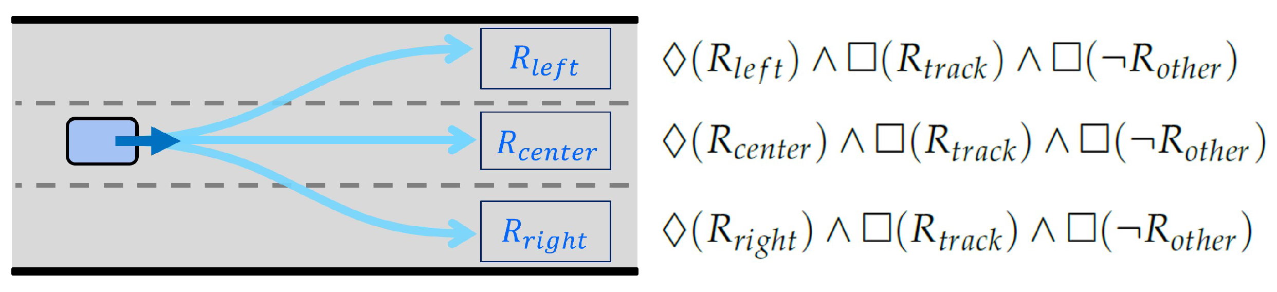
5.3. Application to an Autonomous Driving Environment

In the dynamic landscape of autonomous driving, reactive planning is paramount for safe navigation. The solution of the proposed network was utilized as the output of the reactive planner. During the evaluation, three Linear Temporal Logic (LTL) formulas were employed (Figure 12):

• ${\varphi }_{left}=◊\left(R_{left}\right)\wedge \square \left(R_{track}\right)\wedge \square (\neg R_{other})$;
• ${\varphi }_{center}=◊\left(R_{center}\right)\wedge \square \left(R_{track}\right)\wedge \square (\neg R_{other})$;
• ${\varphi }_{right}=◊\left(R_{right}\right)\wedge \square \left(R_{track}\right)\wedge \square (\neg R_{other})$.

Here, $R_{left}$, $R_{center}$, and $R_{right}$ denote temporal goal regions, $R_{track}$ denotes the region inside the track, and $R_{other}$ denotes regions occupied by other vehicles. The formula ${\varphi }_{left}=◊\left(R_{left}\right)\wedge \square \left(R_{track}\right)\wedge \square (\neg R_{other})$ signifies the goal to “reach the region $R_{left}$ while remaining within the track region ($\square \left(R_{track}\right)$) and avoiding collisions with other vehicles ($\square (\neg R_{other})$).”

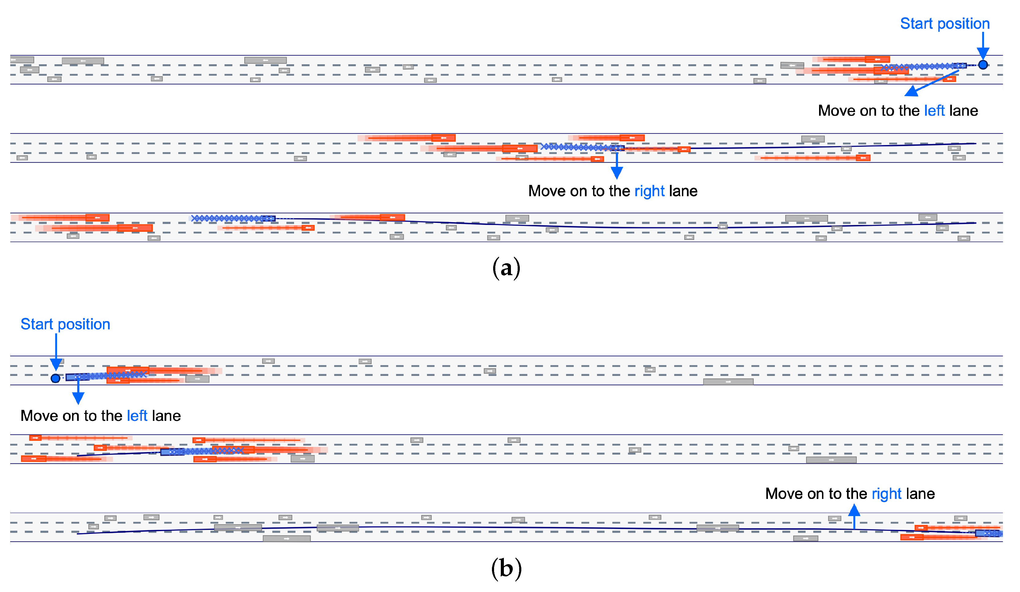
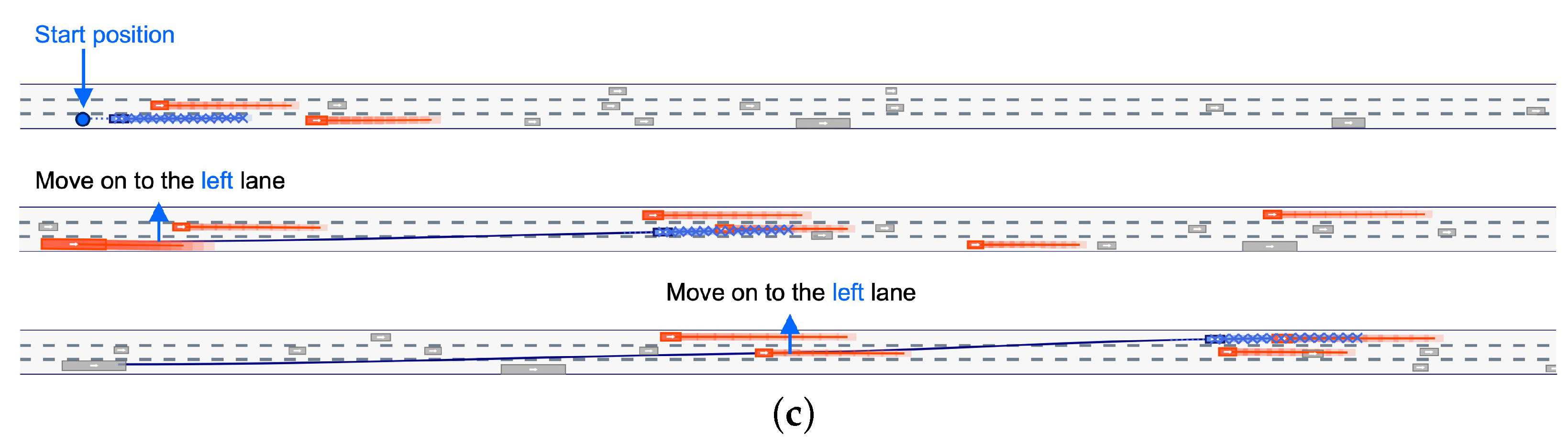
For each situation, one of the three LTL formulas was selected, and a control sequence corresponding to the chosen LTL formula was generated. Generally, ${\varphi }_{center}$ is selected, with the lane-changing formulas (${\varphi }_{left}$, ${\varphi }_{right}$) being chosen only in specific times.

Figure 13 presents snapshots from the experiment conducted using the highD dataset [38]. The decision to change lanes was made at specific points in time, allowing up to two lane changes per trial. In the figure, the ego vehicle is marked in blue, with its trajectory indicated by a blue line. Each subfigure contains three snapshots from a single trial, with lane change points indicated by arrows.

Comparison experiments with other deep learning methods were conducted. We selected a test dataset from the highD dataset, which includes 60 tracks. The test dataset specifically included track IDs 10, 20, 30, 40, and 50, which were not used during the training stage. For each track, 200 trials were conducted. Each trial involved controlling a different vehicle, ensuring fairness by using the same vehicle for each method. The success metric was defined as the controlled vehicle reaching the end of the lane without incidents (collisions or going off track).

Table 2. Success ratio (percentage) in the highD dataset.

	Track ID: 10	Track ID: 20	Track ID: 30	Track ID: 40	Track ID: 50
MLP	90.0	89.5	86.5	85.5	88.0
Seq2Seq-LSTM	91.0	90.0	89.0	88.0	89.5
TCN [41]	90.5	89.5	87.5	86.5	88.5
TFN [13]	93.5	92.0	91.0	90.0	92.5
Proposed	94.5	92.5	91.5	91.0	93.0

summarizes the results. The proposed method exhibited superior safety compared to other deep learning methods.

6. Conclusions

This study presents a pioneering path-planning approach that effectively integrates co-safe Linear Temporal Logic (LTL) specifications with an end-to-end deep learning architecture. Our method stands out for its ability to generate near-optimal control sequences by combining a Transformer encoder, which is informed by LTL requirements, with a Variational Autoencoder (VAE) enhanced by Gaussian Mixture Model (GMM) components. This architecture adeptly handles the complexities of path planning by accommodating a diverse range of tasks and managing inherent uncertainties within these processes.

Empirical evaluations demonstrate the significant advantages of our approach over existing deep learning strategies. In our experiments, the proposed method consistently outperformed other methods in terms of safety and efficiency, particularly in the context of autonomous driving scenarios using the highD dataset. Our approach achieved higher success rates in reaching the end of the lane without incidents, indicating its robustness and reliability. Furthermore, the method’s adaptability and scalability were highlighted through various test cases involving both synthetic and real-world data.

The results confirm the method’s suitability for a wide array of systems, significantly enhancing path-planning processes. By effectively addressing the challenges posed by complex environments and logical constraints, our approach offers a robust solution for diverse robotic applications.

Looking ahead, we aim to apply our methodology to more challenging high-dimensional path-planning problems, particularly those involving additional logical constraints and intricate operational contexts, such as multi-joint robotic manipulations. Expanding our focus to these areas is expected to yield further valuable insights into robotics and automation, enhancing the sophistication and efficiency of path-planning techniques.

The integration of deep learning with logical frameworks in our study represents a significant advancement in robotic path planning, paving the way for more complex and effective mission executions in the future.