Ship Classification Based on AIS Data and Machine Learning Methods

Abstract

AIS ship-type code categorizes ships into broad classes, such as fishing, passenger, and cargo, yet struggles with finer distinctions among cargo ships, such as bulk carriers and containers. Different ship types significantly impact acceleration, steering performance, and stopping distance, thus making precise identification of unfamiliar ship types crucial for maritime monitoring. This study introduces an original classification study based on AIS data for cargo ships, presenting a classifier tailored for bulk carriers, containers, general cargo, and vehicle carriers. The model’s efficacy was tested within the Changhua Wind Farm Channel using eight classification algorithms across tree-structure-based, proximity-based, and regression-based categories and employing standard metrics (Accuracy, Precision, Recall, F1-score) to assess the performance. The results show that tree-structure-based algorithms, particularly XGBoost and Random Forest, demonstrated superior performance. This study also implemented a feature selection strategy with five methods, revealing that a model trained with only four features (three ship-geometric features and one trajectory behavior feature) can achieve high accuracy. Conclusively, the classifier effectively overcame the challenges of limited AIS data labels, achieving a classification accuracy of 97% for ships in the Changhua Wind Farm Channel. These results are pivotal in identifying abnormal ship behavior, highlighting the classifier’s potential for maritime monitoring applications.

1. Introduction

Offshore wind power is an eco-friendly and sustainable energy source that aids in cutting carbon emissions, mitigating climate change, and conserving natural resources. Taiwan’s western coast offers ample wind energy resources, ideal for offshore wind power generation. This could potentially replace nuclear and thermal power generation and be a key focus in future energy supply development. The Changhua Offshore Wind Farm is located in the maritime region adjacent to Changhua, situated north of the Pescadores Channel (Penghu Channel), known for its significant maritime traffic. The competent authority delineated the ship’s navigation channel through the Changhua Offshore Wind Farm, instituted a traffic separation scheme, and established a Ship Traffic Service (VTS) for effective monitoring and management. The VTS offers real-time wind farm data to ships, monitors ship navigation, issues early crisis alerts, and provides guidance when needed, ensuring coordinated navigation and preventing ship collisions.

To enhance maritime traffic management, the International Maritime Organization (IMO) made it mandatory in 2004 for international sailing ships with 300 gross tonnage or more and all passenger ships to install AIS (Automatic Identification System) equipment. AIS is an automated tracking system on ships that identifies and shares data with nearby ships, AIS shore stations, satellites, and other equipment. This data enables ships and coast stations to access navigation information about all ships in the monitored waters. AIS data aids in offering navigation guidance, ensuring ships follow safe routes and maintain distances from each other while avoiding collisions with offshore wind power facilities. This is accomplished using automatic ship alerts or intervention by VTS operators.

In recent years, AIS spatio-temporal data has found extensive applications in maritime traffic analysis, improving maritime safety, detecting atypical ship behavior, enhancing situational awareness, aiding in rescue operations, monitoring marine pollution, and supervising ships, among other related fields [1]. Real-time AIS data simplifies ship status identification. Additionally, it can extract ship navigation traits from historical records to construct crucial maritime traffic or ship behavior models for maritime monitoring and abnormal behavior detection [2]. However, within extensive AIS records, anomalies and inaccuracies often remain concealed. Notably, some ships intentionally evade detection and engage in illicit activities, including disabling transponders, manipulating location data, or sending false identification information, such as ship type [3]. Determining a ship’s precise type in real-time or historical AIS data can be demanding, leading to challenges in maritime surveillance and hindering subsequent data exploration and analysis.

AIS ship-type codes classify ships as fishing ships, passenger ships, cargo ships, or tankers. In contrast, general merchant ships such as bulk carriers, container ships, general cargo ships, and vehicle carriers are all grouped under the broad category of cargo ships without further differentiation. Ship types have a substantial impact on maneuverability, influencing factors such as acceleration, heading stability, steering performance, and stopping distance. For instance, container ships generally exhibit better maneuverability than bulk carriers. This necessitates crew and Ship Traffic Service (VTS) operators to anticipate ship behavior in busy and confined areas. Hence, accurate ship classification and identification become vital [4].

Traditional maritime navigation supervision relies on charts and radar, driven by the operator’s experience. In recent years, the development and innovation of artificial intelligence (AI) technologies, including machine learning and deep learning, have supplied advanced tools for AIS data mining. Utilizing AI algorithms to extract maritime traffic features from AIS data and develop surveillance systems is a crucial research area. Some studies have successfully employed machine learning methods for ship classification, such as Support Vector Machine, K-Nearest Neighbor, and Convolutional Neural Networks. Ship-type classification, as a foundational aspect of maritime supervision and safety, aids in classifying ships and enhancing maritime surveillance applications.

This study aims to create a ship-type classifier for the Changhua wind farm channel using AIS data, focusing on the early detection of abnormal ship behavior in the intelligent maritime safety system. Key contributions of this study are the following:

• In ship classification and identification, this study performed extensive feature extraction on AIS data from the Changhua Wind Farm Channel. This process yielded a set of 14-dimensional features, which encompassed various ship-geometric and trajectory behaviors such as speed, heading, and lateral deviation distance. These findings significantly enhanced the ship classification features, contributing to a more comprehensive understanding of maritime activities in the specified area.
• This study utilized machine learning algorithms on AIS data to develop a ship classification framework, which included data collection, preprocessing, feature engineering, and evaluation of classification algorithms with optimization. The evaluation results showed that tree-structure-based classifiers, particularly XGBoost and Random Forest algorithms, outperformed other methods in classification metrics for this problem.
• This study also implemented a feature selection strategy using five different methods, demonstrating that a ship classification model trained with just four features—three ship-geometric features (width, perimeter, and bridge position ratio) and one trajectory behavior feature (speed)—can achieve high classification accuracy.
• This study explores the significance of the feature “Bridge Position Ratio (BP)” in the context of ship classification, attributing its importance to the distinctive features exhibited by bridges across different ship types.

2. Related Work

According to the type of data used, there are two categories of research on ship-type classification: one is based on image data, such as ship photos taken in ports, aerial or satellite images, and the other is based on information such as speed and heading of AIS data. The image-based ship-type recognition method [5,6,7] mainly uses unsupervised learning convolutional neural networks (CNN) to identify the basic features of ship images. However, optical sensors cannot be used at night or in bad weather conditions, and the image-based ship-type recognition system has become ineffective. Xu et al. [7] classifying ships based on Synthetic Aperture Radar (SAR) images is a complex fine-grained problem, still lacking sufficient study and posing significant challenges. SAR image resolution still makes it difficult to identify bulk carriers, container ships, and oil tankers with similar scale and outline. Another approach focuses on the development of algorithms and models in the field of ship classification based on AIS data. The data classifies ships according to their ship-geometric and trajectory behavior features (such as time, trajectory coordinates, ship length, ship width, draft, speed, course, etc.). The ship features contained in AIS data can make up for the shortcomings of traditional radar and optical identification. However, ship feature data also has problems, such as human errors (intentional or unintentional) and missing ship-type information, which still need further research.

One of the features extracting the procedures of ship classification methods based on AIS data is the conversion of the AIS spatiotemporal data of ship trajectories into graphic data and the use of graphical recognition algorithms to train the ship-type recognition system [8,9,10]. Luo et al. [8] introduced an image-based ship classification model that visualizes latitude and longitude in a scatter plot, maps track point speeds to color, and includes a coastline outline for trajectory image data. This model employs a deep residual network for training and addresses a ship-type classification problem encompassing cargo ships, fishing boats, container ships, oil tankers, and passenger ships. Experimental testing achieved a 92% accuracy rate, surpassing other methods in classification performance. Nevertheless, there remains potential for improvement in classifying passenger ships and tankers. Referring to Li et al. [9], the ship trajectory data exhibits time–space domain features and a non-Euclidean structure. This data is transformed into graph data with vertices and edges, resulting in an 82.7% accuracy in classifying different ship types (fishing boats, passenger ships, tankers, and containers) using trajectory graphic data. Yang et al. [10] used AIS data to generate ship trajectory images, including static, normal navigation, and maneuvering states. Apply a Convolutional Neural Network (CNN) for ship classification, discerning eight ship types (fishing boats, tugboats, sailing boats, leisure boats, passenger ships, cargo ships, crude oil/oil product ships, and others) based on ship track images. The corresponding AIS ship-type codes are 30, 31, 36, 37, 60, 70, 80, and 90, achieving an 87.5% accuracy rate.

Another method for feature extraction in ship classification directly derives geometric and motion features from AIS static and dynamic data, bypassing the need for graphic data conversion. Then, the features are used as learning data for the ship classification model [1,2,4,11,12,13]. Wang et al. [12] utilized the original AIS static message, incorporating six fields: A, B, C, D, draft, and the ship-type code. The data was used to derive ship attributes, including length, width, draft, and geometric features such as aspect ratio, perimeter, and area. Using the random forest method, five ship types—passenger ships, tugboats, oil tankers, fishing boats, and cargo ships—were identified with an accuracy rate of 86.14%. The results show that static trajectories and ship shape characteristics may be similar between certain types of ships, such as cargo ships and cruise ships. Only extracting static features is not enough to construct a classification model capable of distinguishing five types of ships. The static and dynamic information of AIS data should be combined to improve the performance of ship-type classification. Yan et al. [1] used space-borne AIS data, which has the advantages of wide coverage, long tracking time, and rich ship types. Static and dynamic information from AIS data were systematically extracted and analyzed thoroughly. In addition to the ship’s length, width, and draft, static features refer to the geometric features proposed by Lang et al. [13], such as naïve perimeter, naïve area, aspect ratio, and shape complex. Trajectory behavior features include ship position, voyage distance, ship speed, and other feature quantities. Based on these two types of features, the random forest model machine learning algorithm is used for five types of ships, including cargo ships, oil tankers, fishing boats, passenger ships, and tugboats, with an accuracy rate of 92.7%. The model test results show that the accuracy rate is improved by combining geometric and trajectory behavior features.

Compared with the method of converting AIS ship trajectory spatiotemporal data into graphic data, it is simpler, faster, and more efficient to extract geometric features and motion behavior features from AIS data directly. It is suitable for real-time maritime navigation safety monitoring systems. Baeg and Hammond [4] proposed a ship classification method for AIS data in Danish waters to solve the problem of missing and tampering with type information in AIS data. Static and dynamic features (ship geometry, motion features, and time features) were extracted from AIS data, the features of the Danish water’s geographical region were integrated, and the ink features of the sketch recognition design were proposed to represent the ship trajectory type. There are a total of 39 features. Various classification algorithms, such as random forests and decision trees, are used for performance comparison. The results and discussion show that Random Forest outperforms other classifiers in classifying AIS data. The classification accuracy of the four ship types can reach 84.05%. In particular, the accuracies of fishing boats and passenger boats were 0.951 and 0.946, respectively, confirming very high results. However, the practical features that distinguish cargo ships from oil tankers must be further explored.

The above review and analysis show that the current research mainly solves the problem of missing and tampering with type information in AIS data. The ship-type classification method aims to confirm the classification of AIS ship-type codes. However, the cargo ships that also belong to the AIS ship-type code 70 include bulk carriers, container ships, general cargo ships, and vehicle carriers, and the ship-type code 80 includes crude oil tankers and oil product tankers. The differences in the maneuverability of various types of ships significantly affect the navigation behavior of ships. Prior to the development of a maritime navigation safety monitoring system by the regulatory authorities, there was an urgent need to develop a ship-type classifier for bulk carriers, container ships, general cargo ships, vehicle carriers, crude oil tankers, or oil product tankers.

3. Data Preparation and Analysis

Due to the widespread use of AIS equipment, the long-term collection of AIS records has become a valuable source of big data for maritime traffic analysis. The AIS data used in this study is collected from AIS receiving stations along Taiwan’s coast, which are managed by the Maritime and Port Bureau, Ministry of Transportation and Communications, Taiwan. The AIS data cover the entire year of 2022, amounting to nearly six billion historical records and a file size of approximately 2 terabytes (TB). However, AIS information is compressed during transmission, and after decoding and restoration as numerical records, each AIS record is discrete with no temporal and spatial connections. Additionally, each AIS record is discrete. Without temporal and spatial connections, a single AIS record provides only a ship’s state at a specific time, limiting its usefulness, which is regrettable. Hence, it is crucial to investigate extracting valuable features from AIS records and converting them into actionable knowledge for maritime decision-making.

3.1. AIS Pre-Processing

AIS is a system aiding ship navigation, with functions like ship identification, information exchange, target tracking, and automatic calculation of CPA and TCPA, etc. These functions enable authorities to monitor ship activity efficiently, improving maritime navigation safety. According to Series [14], 27 distinct AIS information types are classified into static, dynamic, and voyage categories, with the primary fields listed in

Table 1. AIS primary fields.

Static Information	Dynamic Information	Voyage Information
Ship name	Position	Draft
Call sign	SOG	ETA
IMO number	COG	Destination
MMSI	True heading	Route plan
Location of position fixing antenna on the ship	ROT	Hazardous cargo
Ship and cargo type	Navigational status

. Among these, MMSI is part of the static information category, and each AIS transceiver has a unique MMSI, enabling the identification of individual ships or devices. AIS data is transmitted every few seconds via two specific digital VHF (Very High Frequency) channels within a confined geographic area. The transmission frequency depends on ship speed and turning rate, with faster and turning ships providing more frequent updates. AIS transponders operate continuously, irrespective of a ship’s location, whether offshore, in coastal or inland waters, or at anchor.

The data quality of AIS significantly affects the performance of ship-type recognition and the classification model. Referring to Tsou [15], this study utilizes big data analysis to cleanse, store, and identify raw data, streamlining the extensive and disorganized digital records. First, the data processing was conducted according to the AIS standard of the International Telecommunication Union (ITU) [14]. The AIS data with apparent abnormalities, such as longitude exceeding 180°, latitude exceeding 90°, etc., was cleared. Secondly, the AIS data is sorted by MMSI and timestamp to obtain the trajectory information for each ship. Next, if a ship lacks data for over 30 min, its speed drops below 1 knot, or latitude and longitude change exceeding 0.01°, the trajectory is split into two sub-trajectories. Furthermore, AIS static and voyage information are prone to manual input errors and omissions, which are more frequent than dynamic information directly sourced from navigation instruments [16]. Consequently, in the data cleaning process, this study must also verify the accuracy of static data. Finally, the static, dynamic, and voyage data of ship platform shape and navigation parameters are extracted, which include MMSI that can identify a single ship, navigation parameters (SOG, COG, THD, Longitude, Latitude), ship-geometric parameters (A, B, C, D, Draught), and the “Record Time” that can create AIS time–space sequences.

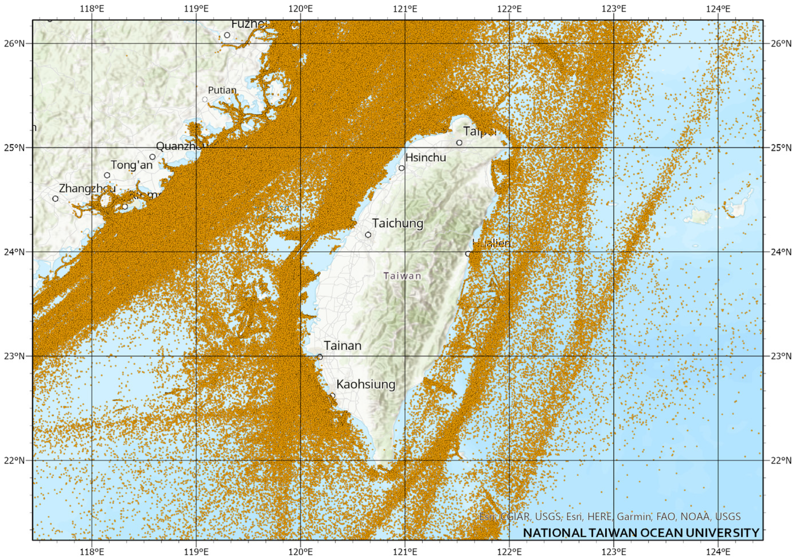
After data pre-processing, this study employed GIS to import AIS data into a map platform, establishing ship navigation trajectories through spatial geometric calculations. This provided a visual representation of the spatiotemporal aspects in AIS data, and spatial statistical analysis was performed to create feature data for subsequent modeling. Figure 1 displays the distribution of AIS data points for ships in the waters around Taiwan on a specific day in 2022. There is a noticeable concentration of AIS signals in the Taiwan Strait, while the Eastern Pacific Ocean has fewer and less dense signals.

3.2. The Changhua Wind Farm Channel

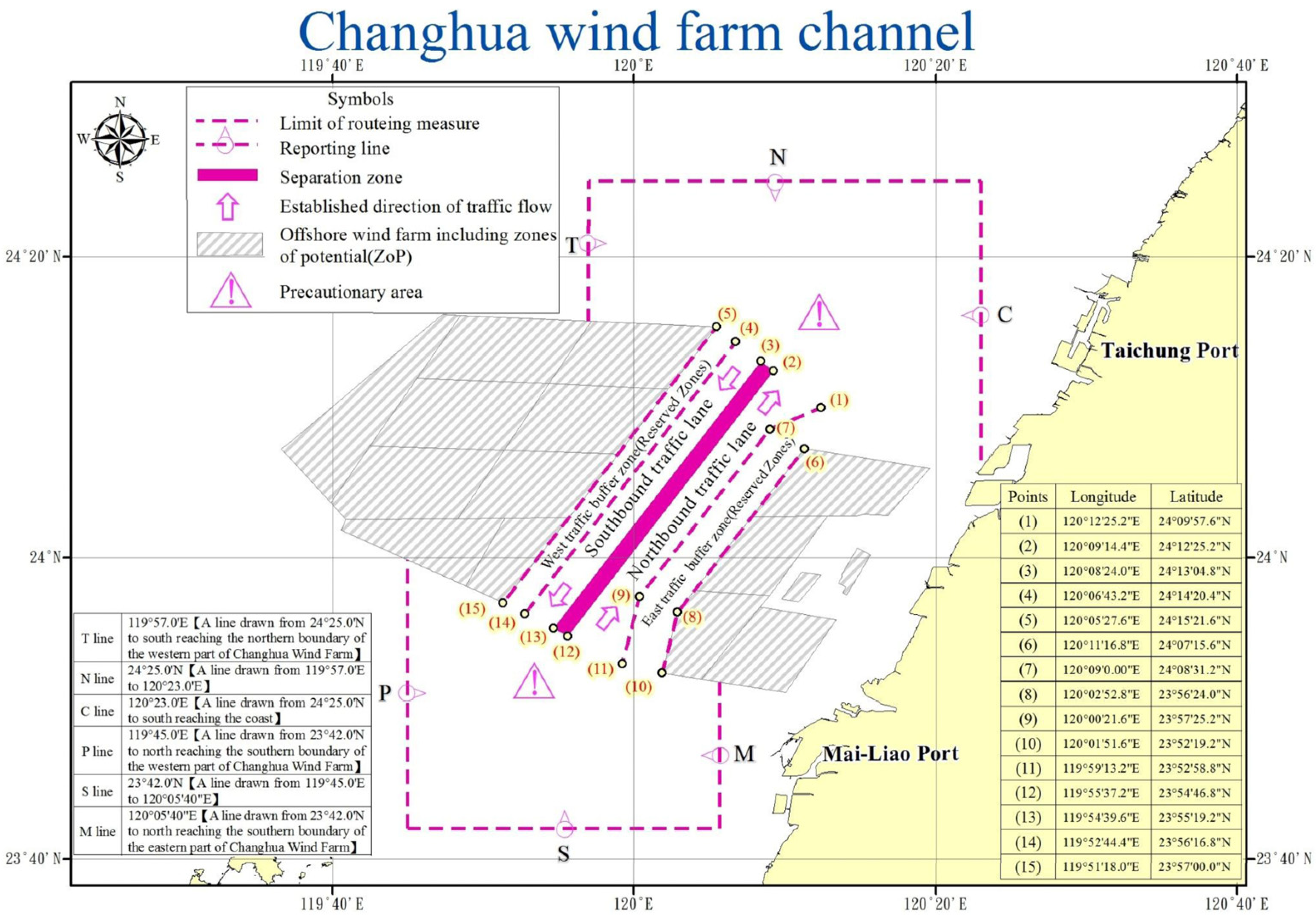
In line with government energy policies, substantial offshore wind farm development is scheduled for Taiwan’s western waters. Changhua offshore waters are the first area for large-scale construction. Therefore, the Changhua wind farm channel was officially implemented in October 2021, the first wind farm channel in Taiwan, as shown in Figure 2. The gray areas on both sides are wind farm locations. A traffic separation system is adopted, according to International Regulations for Preventing Collisions at Sea (COLREGs) [17], which consists of a southbound traffic lane, a northbound traffic lane, a separation zone, and buffer zones on both sides. The width of the northbound and southbound channels is 2 nm.

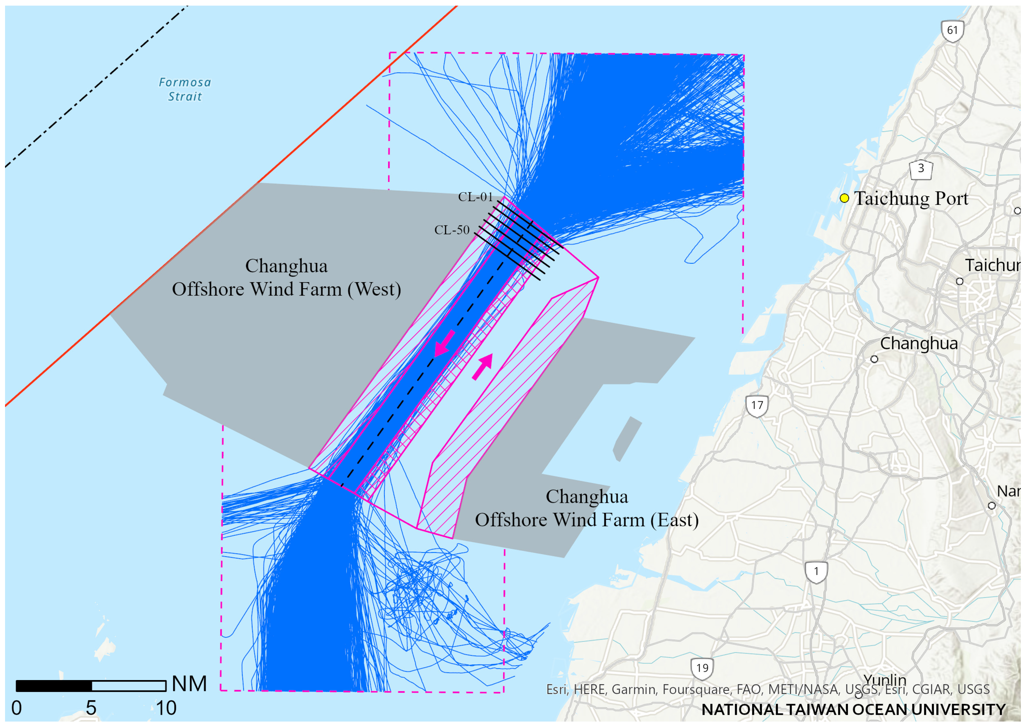
Changhua Offshore is a vital water area connecting Kaohsiung Port with Taipei and Keelung Ports. It is also an international shipping route connecting Northeast Asia to Southeast Asia. Many ships pass through this area, and the traffic is very heavy. Figure 3 shows the maritime traffic density map before and after the implementation of the Changhua wind farm channel. Before the implementation of the channel, the ship tracks spread widely, and the southbound and northbound tracks overlapped. After the channel implementation, most ship tracks are concentrated in the southbound and northbound lanes, with only a few offshore wind farm construction ships, maintenance ships, and some fishing boats crossing these lanes. The Maritime and Port Bureau, MOTC, has established the “Changhua VTS” to surveil and manage traffic lanes for safe navigation. On average, there are at least 150 ships passing through this channel every day, and most of the ships can sail in compliance with the channel regulations.

To assist the Ship Traffic Service (VTS) operation, tracking ship behavior, anomaly detection, and warnings prediction are crucial topics in developing modern intelligent waterway systems [18]. Nevertheless, a prerequisite for setting up this system is comprehending ship types, their distinct maneuvering capabilities, and cargo characteristics across various ship types. This study primarily creates a ship classification algorithm for the Changhua wind farm channel, focusing on the cargo ship classification problem. The AIS trajectory data with ship-type codes between 70 and 79, indicating cargo ships, is extracted based on reporting lines on the north and south sides of the channel. Figure 4 displays some ship trajectories along the southbound traffic lane.

In order to analyze the navigation characteristics of ships in the channel effectively, the data representing the track line are normalized. Refer to Huang et al. [19] to create a set of analysis gate lines perpendicular to the southbound traffic lane in the head section of the channel. The distance between two adjacent crossing-line is taken as a constant of 100 m, and there are 50 crossing-lines in total. Through the spatial analytical calculations, each trajectory passing through the channel intersects with the crossing lines. The ship’s lateral position, speed, and heading data, provided by the AIS information, are recorded at each crossing line so that the temporal and spatial distribution of the training data is consistent.

In this study, a data-driven supervised learning approach is applied to differentiate between four cargo ship types: container ships, bulk carriers, general cargo ships, and vehicle carriers. Each ship’s registration ship type and ship dimensions (length and width) were individually obtained from the internet using MMSI to create a training and testing dataset for ship classification. The sample quantities for the four ship types are detailed in

Table 2. Number of cargo ship’s trajectories by the four types of ship.

Ship Type	Bulk Carrier	Container Ship	General Cargo	Vehicle Carrier	Total
Quantity	4286	3896	1243	360	9785

.

3.3. Feature Extraction

Selecting the appropriate features is crucial for classifier performance and has a significant impact. Some papers have already introduced various features for classifying ship types, including motion behavior and geometric features [4]. Kraus et al. [20] extracted geographical features, such as the distance to the coast and to classify fishing boats, cargo ships, and oil tankers. Yan et al. [1] extracted the ship geometric features like length, width, and shape complexity to distinguish fishing boats, cargo ships, passenger ferries, oil tankers, and tugs. Moreover, Sheng et al. [2] derived trajectory features from the kinematic pattern to classify fishing boats and cargo ships. Baeg and Hammond [4] introduced an innovative method using ink features designed for sketch recognition to quantify ship trajectory characteristics, enabling the differentiation of fishing boats and cargo ships, as well as passenger ferries and oil tankers.

Previous research results have indicated the potential of using multiple features for ship-type classification. Some features and classifiers have been employed for classifying diverse ship types, including fishing boats, tugs, cargo ships, passenger ferries, and oil tankers. These ship types in AIS data are distinguished by unique codes, such as 30, 31–32, 60–69, 70–79, and 80–89, respectively. To enhance the navigation safety and efficiency of maritime supervision, this study aims to develop a ship-type classifier based on normal navigation behavior models for specific cargo ships (bulk carriers, container ships, general cargo ships, and vehicle carriers) within the cargo ship category numbered 70–79. Kraus et al. [20] classified ship types using ship-geometric and trajectory behavior features from AIS data. Ship-geometric features include parameters like ship length, width, perimeter, area, aspect ratio, and shape complexity extracted from AIS static information. Trajectory behavior features encompass parameters related to ship movement, including latitude, longitude, speed, heading, turning rate, and trajectory extracted from AIS dynamic information.

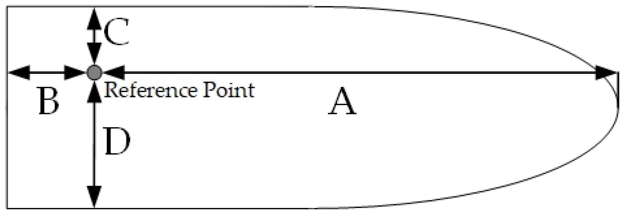
One of the goals of this study is to test and select ship classification features based on AIS static and dynamic data and suggest precise and efficient classification methods. In AIS static information, the data fields A, B, C, and D represent the distances from the antenna or reference point O to the bow, stern, port side, and starboard side of the ship, as shown in Figure 5. Ship length and ship width features can be calculated using the following equations:

$$\{\begin{array}{l}L=A+B\\ W=C+D\end{array}$$

(1)

where L represents the ship’s total length, and W represents the ship’s width.

The novel parameter introduced in this study, which represents the ratio of bridge position to the ship’s length, has been named “Bridge Position Ratio”. Because most antenna positions or reference O points are located on the bridge, this value can be obtained from field A. This parameter is essential because, due to the influence of the shipbuilding industry, large or ultra-large container ships (≥18,000 TEU) adopt the form of double bridges, and the antenna or reference O point will be set on the front bridge, which is different from traditional container ships. Generally, container ships still have space for stacking containers behind the bridge. Still, the main loading positions of bulk carriers and general cargo ships are in front of the bridge, so the value A of bulk carriers and general cargo ships will be closer to the ship’s length. This study also encompasses parameters such as perimeter, area, aspect ratio, and shape complexity, references employed by Wang et al. [5], Lang et al. [13], and Yan et al. [1]. The definitions are provided in the following equations:

$$\{\begin{array}{l}{P}_s=2\times \left(L+W\right)\\ A_s=L\times W\\ A_R=\frac{W}{L}\\ C_s=\frac{{(L+W)}^2}{L\times W}\\ B_P=\frac{A}{L}\end{array}$$

(2)

where P_s represents Naive Perimeter, A_s represents Naive Area, A_R represents Aspect Ratio, C_s represents Shape Complexity, and B_P represents Bridge Position Ratio.

In addition to the seven ship-geometric features in this study, trajectory behavior features were extracted from AIS dynamic information to enhance the accuracy of ship-type classification. In processing dynamic information data, through the crossing-line method in Section 3.2, the dynamic information initially recorded on the AIS is converted to a specific crossing-line dataset, and the coordinate data (longitude and latitude) are converted into the lateral position of each crossing-line. With the centerline of the southbound lane as the reference point, positive values signify a right-side deviation, while negative values indicate a left-side deviation. In addition to reducing data dimensionality, this approach establishes a consistent standard for subsequent training data. Fifty sample data points were extracted from each ship’s trajectory, calculating six variables for each trajectory: the median values of ship speed, course, and lateral position (denoted as S_med, C_med, and T_med, respectively), as well as the interquartile range (IQR) (represented as S_iqr, C_iqr, and T_iqr). These variables capture the speed, course, and position deviation of each trajectory, with their respective variability ranges representing the navigational characteristics of the ships. Additionally, this study includes the ship’s draft as a feature. Due to their smaller size, general cargo ships typically have shallower drafts compared to bulk carriers and container ships. Moreover, container ships typically have significantly shallower drafts compared to bulk carriers of similar length.

This study extracted a total of 14 features from 9785 ship trajectory samples. The feature vector can be expressed as follows:

$$f=\left[L, W, D_r, P_s, A_s, A_R, C_s, B_P, T_{med}, S_{med}, C_{med}, T_{iqr}, S_{iqr}, C_{iqr}\right]$$

(3)

In the above formula, draft (D), median of Transverse deviation from channel central line (T_med), median of speed over ground (S_med), median of course over ground (C_med), Interquartile range of Transverse deviation (T_iqr), Interquartile range of speed over ground (S_iqr), Interquartile range of course over ground (C_iqr).

This study collected 9785 trajectory data points from ships navigating southbound in the Changhua Wind Farm Channel since 2022. These ships are categorized into four types: bulk carriers, container ships, general cargo ships, and vehicle carriers. Statistics for ship-geometric and trajectory behavior features are detailed in

Table 3. Statistics of ship-geometric features.

	L	W	Dr	Ps	As	AR	Cs	BP
Mean	200.1	31.3	8.7	462.8	6838.3	6.39	8.55	0.79
std	64.6	9.5	2.1	147.4	4269.1	0.62	0.61	0.16
Minimum	40.0	4.0	2.0	96.0	228.0	3.33	5.63	0.00
25%	160.0	25.0	7.3	370.0	4004.0	6.00	8.17	0.78
50% (Median)	190.0	32.0	8.6	444.0	6048.0	6.26	8.42	0.85
75%	229.0	33.0	9.8	522.0	7425.0	6.57	8.72	0.87
Maximum	400.0	65.0	25.5	924.0	24,800.0	15.91	17.97	1.00

and

Table 4. Statistics of trajectory behavior features.

	Tmed	Smed	Cmed	Tiqr	Siqr	Ciqr
Mean	−172	13.2	215.2	169	0.2	2.2
std	803	2.8	3.2	207	0.2	2.8
Minimum	−10,773	2.6	193.9	1	0.0	0.0
25%	−660	11.3	213.7	53	0.1	0.7
50% (Median)	−170	12.9	215.0	113	0.1	1.3
75%	290	15.0	216.5	212	0.2	2.5
Maximum	3575	23.4	254.0	3298	9.3	45.2

, respectively.

Table 3 displays the statistical characteristics of ship-geometric features. The statistics for the ship’s length show an average length of 200.1 m and a median length of 190 m. The slightly lower median compared to the mean suggests that the distribution of the ship’s lengths is relatively balanced, with no severe outliers significantly affecting the mean. The standard deviation (64.6 m) compared to the IQR (139 m) indicates a wide dispersion in the ship’s lengths, and there is significant variability in the lengths of ships within the middle 50% of the data range. The statistics for draft reveal an average draft of 8.7 m, which is very close to the median draft of 8.6 m. Most ships have draft depths falling within the range of 7.3 to 9.8 m. The similar IQR (2.5 m) and standard deviation (2.1 m) further suggest high data centrality, with minimal differences in draft depths among the majority of ships. For most geometric features of ships, there is only a slight difference between their mean and median values. However, certain features such as W, A_s, A_R, C_s, and B_P exhibit smaller interquartile ranges compared to the standard deviation, implying the presence of a few outliers or anomalies that contribute to increased overall data variability.

Table 4 displays the statistical measures of trajectory behavior characteristics. The trajectory speed (S_med) statistics show an average speed value of 13.2 knots, closely aligned with the median of 12.9 knots. This indicates a relatively balanced distribution of sailing speeds, with minimal impact from extreme values. The IQR of 3.7 knots, larger than the standard deviation of 2.8 knots, suggests that most ship speeds are distributed within a narrow range. The average speed variation range (S_iqr) is 0.2 knots with a median of 0.1 knots and a standard deviation of 0.2 knots. The low average and standard deviation indicate that most trajectories exhibit a very narrow range of speed variation, implying stable speeds. The maximum value of 9.3 knots points to the presence of outliers, suggesting more considerable speed variations under certain conditions or for specific ship types. The trajectory course (C_med) statistics show an average course value of 215.2 degrees, closely matching the median of 215 degrees. The IQR of 2.8 degrees, nearly equivalent to the standard deviation of 3.2 degrees, indicates high centrality in the dataset. This suggests that most ships maintain a stable course with minimal directional changes, adhering to navigation guidelines. The average course variation range (C_iqr) is 2.2 degrees with a standard deviation of 2.8 degrees. The IQR of 1.3 degrees and a standard deviation of 2.8 degrees in C_iqr reflect a more comprehensive range of changes in some trajectories, indicative of diverse navigational behaviors in complex channel environments or adverse weather. Regarding the lateral offset position (T_med), the average value is −172 m, and the median is −170 m. This suggests that most ships’ lateral offsets are to the left of the channel’s centerline within a relatively fixed range. The IQR of 950 m and a standard deviation of 803 m show that ships effectively maintain their intended paths within the 2-nm-wide channel. However, extreme values (minimum −10,773 m, maximum 3575 m) indicate significant lateral deviations in some cases, possibly due to emergency maneuvers, strong wind and wave effects, or navigational errors. The average lateral offset variation range (T_iqr) is 169 m with a standard deviation of 207 m, highlighting significant differences in lateral deviation across trajectories. This variability may reflect responses to channel width, traffic density, or environmental factors. The maximum value of 3298 m suggests significant lateral deviations under special navigational circumstances.

In summary, the statistical data on speed, course, and lateral offset variations reveal high consistency and predictability in ship speeds and courses on the channel. Most ships maintain a stable course and lateral offset, indicating adherence to navigation guidelines and channel stability. However, the data also imply potential speed and course variations under specific conditions. These insights are crucial for channel management and maritime safety strategy development, highlighting the need for tailored navigational protocols.

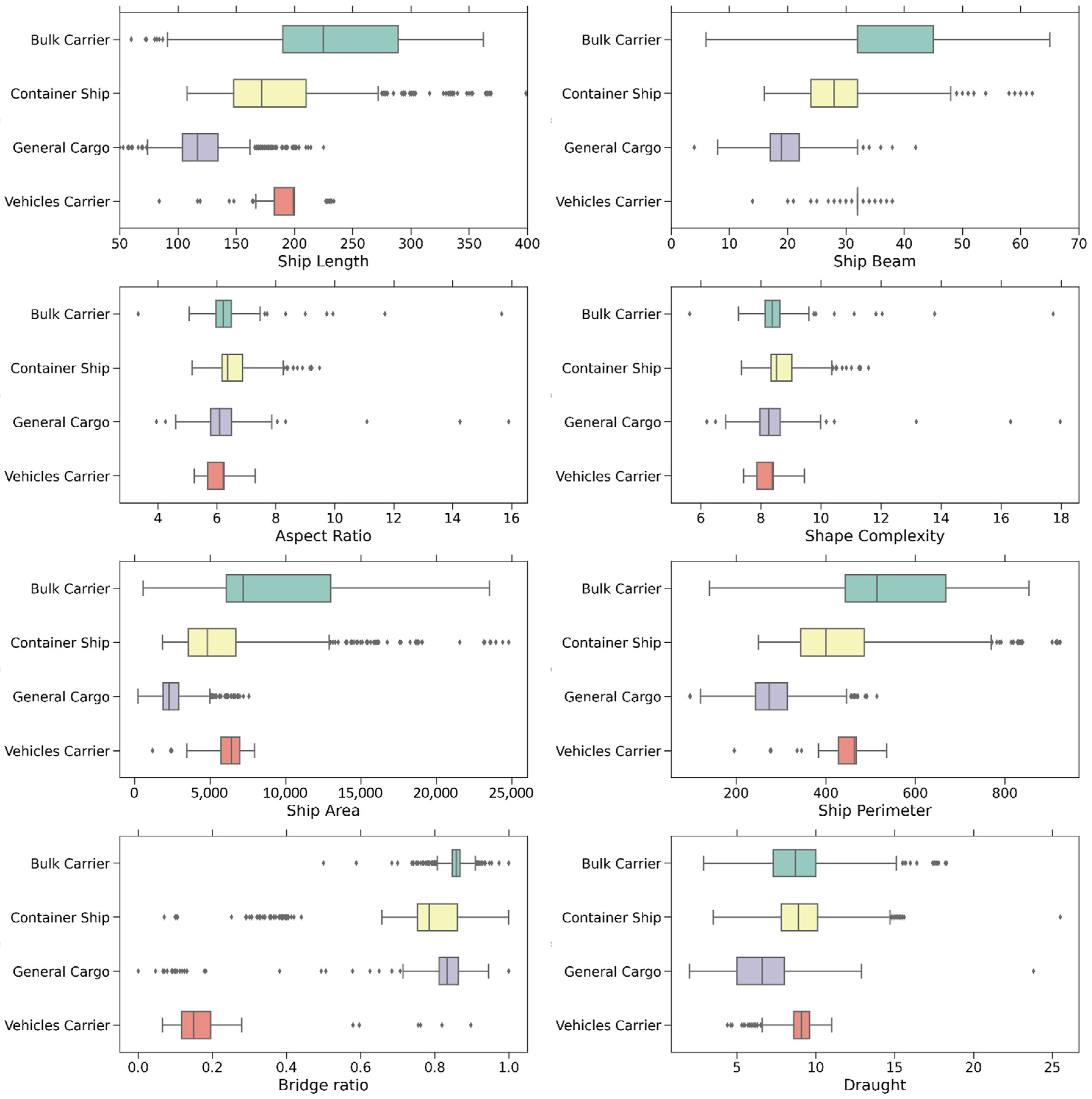
Subsequently, this study further divided the data into four ship types and created box plots for comparative analysis. Figure 6 presents the ship-geometric features of these four ship types, while Figure 7 illustrates their trajectory behavior characteristics in the southbound traffic lane. Bulk carriers, container ships, and general cargo ships exhibit significant differences in length, width, area, and perimeter. Bulk carriers, larger in tonnage, typically show more extraordinary lengths and widths (approximately 180–300 m in length, 30–45 m in width), with outliers indicating the presence of smaller ships. In contrast, general cargo ships, usually smaller in tonnage, display shorter lengths and narrower widths (approximately 100–150 m in length, 15–25 m in width), clustering within a more compact range. The IQR and the distribution of outliers for general cargo ships are markedly different from the other three ship types. Vehicle carriers, while similar in principal dimensions to other types, differ distinctly in bridge position ratio (B_P), with bridges often located near the bow, as opposed to the stern placement in other cargo ships. Container ships, typically medium-sized and concentrated in the 150–220 m range, include outliers representing significantly larger ships, such as ultra-large container ships (≥18,000 TEU) with double bridges. However, the aspect ratio (A_R) and shape complexity (C_s), indicators of ship maneuverability, overlap considerably among the four types.

Regarding trajectory behavior characteristics, the speeds of container ships and vehicle carriers mainly range between 14 and 18 knots, higher than the 9–13 knots range of bulk and general cargo ships. However, the trajectory course and lateral position distribution are similar among all four ship types, showing only minor variations. The majority of ships maintain courses within a 2-degree deviation from the traffic lane direction, and their lateral positions are within a 0.5 nm range on either side of the traffic lane’s centerline. This distribution suggests that most ships adhere to channel navigation guidelines, with outliers indicating anomalies in navigation characteristics such as speed, course, or position.

4. Experimental Results and Discussion

All numerical experiments in this study were implemented using Python 3.8 under a Windows 10 environment. The classification algorithm was provided by Scikit-learn Class to evaluate the extracted features for ship-type classification. After calculating the statistical measures detailed in the previous section, ship-geometric and trajectory behavior features were extracted. Subsequently, normalization was applied to all samples using the quartiles and the IQR for each feature. The lower quartile value was scaled to 0, while the upper quartile value was scaled to 1. The classification target was then transformed into four discrete values, with bulk carriers assigned 0, container ships given 1, general cargo ships given 2, and vehicle carriers posted 3. Furthermore, this study employed standard classifier evaluation metrics, including Accuracy, Precision, Recall, and the F1-score, to assess the model’s performance in classifying the four ship types. The relevant calculation is shown in Equation (4). Accuracy is the most frequently utilized metric in classification problems, quantifying the proportion of correctly predicted instances out of the total predicted samples. Nevertheless, in the case of imbalanced datasets, relying solely on Accuracy can yield misleading assessments, emphasizing the importance of considering additional scores. Precision emphasizes evaluating how many of the actual positive instances are accurately predicted among all the predicted positives. Conversely, Recall assesses how many positive samples are correctly predicted as positive. The discussion in this chapter is as follows:

$$\begin{array}{l}Accuracy=\frac{TP+TN}{TP+TN+FP+FN}\\ Precision=\frac{TP}{TP+FP}\\ Recall=\frac{TP}{TP+FN}\\ F_1-score=\frac{2\times Precision\times Recall}{Precision+Recall}\end{array}$$

(4)

4.1. Classification Model

In the realm of machine learning, particularly in supervised learning, no single algorithm can consistently excel in every problem, as its performance is contingent on data features and structure. Hence, it becomes imperative to assess various algorithms for a given problem and gauge their performance using test datasets to pinpoint the most suitable one. In this study, to confirm the efficiency of the extracted features for ship classification in AIS data, this study conducted experiments with eight well-established supervised machine learning algorithms for evaluation: Logistic regression (LR) [21], Decision Tree (DT) [22], K Nearest Neighbor (KNN) [23], Linear Discriminant Analysis (LDA) [24], Gaussian Naive Bayes (GNB) [25], Support vector machines (SVM) [26], Random forest (RF) [27], eXtreme Gradient Boosting (XGBoost) [28]. These algorithms have all been widely used for classification problems.

The eight classification algorithms can be grouped into three main categories: tree-structure-based, proximity-based, and regression-based. DT, RF, and XGBoost belong to the category of tree-structure-based classification algorithms. DT utilizes a simple tree structure with conditional classifiers to handle classification problems, constructed by successively dividing the dataset based on feature criteria determined through information entropy and information gain. Advantages of DT include minimal computation for data classification, the ability to handle both continuous and discrete values, and ease of understanding and interpretation. DT does not require feature normalization, can reasonably take missing values, and is not significantly affected by outliers. However, it can be less effective with too many categories and insufficient data and is prone to overfitting.

RF improves upon DT by generating multiple decision trees, each using a subset of features and data, with the final result determined by majority voting. This approach reduces overfitting and biases inherent in individual trees. Nevertheless, RF has higher training or prediction time complexity than DT, but its efficiency is improved since each tree can run in parallel. The space complexity also increases with the number of trees, particularly when each tree is more complex. The space and time required for training increase with the number of decision trees in the random forest. In contrast, XGBoost builds sequential decision trees, learning from previous mistakes and increasing weight in subsequent trees. It controls model complexity to prevent overfitting, with a higher time complexity during training as trees are built sequentially. XGBoost performs pruning during training, generally making it more efficient than RF. Its space complexity depends on the number and size of trees built.

KNN is a classification algorithm based on proximity. It classifies or regresses a new sample by finding the nearest K neighbors and establishing it on the labels of these neighbors. It requires calculating the distance between the test sample and each training sample and storing the entire training dataset. Its time and space complexity are proportional to the number of training samples and features. GNB is a probabilistic classifier that assumes features follow a Gaussian distribution. It uses Bayes’ theorem to compute each type’s probability of feature values. Then, the test sample is classified into the class with the highest chance, which is the probability distribution closest to the model in terms of probabilistic distance. Therefore, to some extent, GNB can be categorized as an algorithm based on proximity. During the training phase, it calculates the mean and standard deviation for each type, with time complexity linearly related to the number of features and data points, and it predicts relatively quickly during the prediction phase. It only needs to store the mean and standard deviation for each feature per category, making its space complexity comparatively lower than KNN.

LR, LDA, and SVM are methods based on regression algorithms. LR, adapted from statistics, calculates the probability of a sample belonging to a category and efficiently classifies sample data with low time complexity, where computational time is linearly related to the number of features and data points. LDA, a supervised learning method for dimensionality reduction, aims to maximize inter-class differences and minimize intra-class variances. Its time complexity is the order of O (nm²), where n represents a number of samples and m represents the dimensions, primarily due to the computation of the covariance matrix and its inverse, which becomes costly in high-dimensional data. SVM classifies data by finding a hyperplane that maximizes the margin between classes. For linear SVM, the time complexity is proportional to the number of features and samples, while the space complexity is proportional to the number of features. All three methods apply to multi-class problems, with LDA requiring more computation time in high-dimensional data, whereas LR and SVM generally perform better in such settings.

In the numerical experiments, the dataset of 9785 ship samples was randomly split into two parts: 75% for training data and 25% for testing data. Next, the classifier models for bulk carriers, container ships, general cargo ships, and vehicle carriers were constructed using eight classification algorithms. All models were trained with 14 features, including both ship-geometric and trajectory behavior features of the ships, using the original default parameters of the algorithms. Afterward, the accuracy, average precision, average recall, and average F1 score of each classifier were computed using the test data, as detailed in

Table 5. Comparison of classifier’s Accuracy, average Precision, average Recall, and average F1-score (14 Features).

Metrics	Tree-Structure-Based			Proximity-Based		Regression-Based
	XGBoost	RF	DT	KNN	GNB	LR	LDA	SVM
Accuracy	0.964 *	0.963	0.912	0.850	0.888	0.852	0.801	0.893
Precision	0.957 *	0.955	0.892	0.832	0.886	0.826	0.795	0.891
Recall	0.953 *	0.952	0.889	0.817	0.852	0.840	0.825	0.869
F1-score	0.954 *	0.953	0.891	0.824	0.863	0.832	0.791	0.879

* represent the highest score among the eight methods.

. The evaluation metrics are calculated with equal weights for different ship types.

Table 5 demonstrates that the proximity-based classification models, such as KNN and GNB, as well as the regression-based models like LR, LDA, and SVM, have relatively lower evaluation metrics. All these metrics fall below 0.9, with SVM having the highest Accuracy and Precision, approximately 0.89, while GNB exhibits the lowest F1-score, falling below 0.8. Tree-structure-based classifiers like DT, RF, and XGBoost generally achieve high evaluation metrics. RF and XGBoost have accuracy above 0.96, with Precision and Recall around 0.95. DT also has Precision above 0.91, while Precision and Recall are slightly below 0.89. The results of each classification algorithm indicate that XGBoost and Random Forest algorithms are the most suitable for the cargo ship classification problem in this study.

Moreover, this study further examines the classification results of the four ship types. Remarkably, XGBoost and RF algorithms exhibit nearly identical classification metric scores, surpassing other algorithms. Hence, the subsequent discussion is grounded in the outcomes of these two classification models. Figure 8 provides a visual representation of the classification confusion matrices for XGBoost and Random Forest algorithms using the test dataset. The “Actuals” represent the actual ship-type labels from the AIS dataset, while the “Predictions” are the classification outcomes of the algorithms. Notably, general cargo ships commonly encounter distinct challenges during the classification procedure, often leading to misidentifications with bulk carriers or container ships; approximately 10% of them are misclassified as bulk carriers, and about 4% are misclassified as container ships. Furthermore, about 2% of bulk carriers are misclassified as general cargo ships, and around 1% are misclassified as container ships. This misclassification can be attributed to the similarities in ship-geometric and trajectory behavior features between bulk carriers and general cargo ships. Although the training and testing datasets for vehicle carriers are the fewest among the four ship types, they have the highest classification metrics. These high metrics can be attributed to the distinctive design of vehicle carriers, with the primary feature being the bridge’s location at the bow of the ship, resulting in an Accuracy of approximately 99%.

4.2. Feature Selection

Feature selection involves reducing the number of input features when creating a classification or prediction model. This process offers several advantages, including the elimination of redundant data, the prevention of excessive noise during training, and a reduction in the risk of overfitting. Reducing the number of features results in simpler algorithms and more efficient model training. This step is essential in machine learning and can substantially enhance models’ predictive or classification accuracy [29].

Table 6. Feature Importance Ranking.

Ranking	Variable Ranking	Correlation Matrix	Built-In Feature Importance		Permutation Importance		RFECV
			(RF)	(XGBoost)	(RF)	(XGBoost)	(RF)	(XGBoost)
1	BP	BP	BP	W	BP	BP	W, Ps, BP	L, W, AR, As, Ps, BP, Smed
2	Smed	W	W	Ps	W	L
3	W	Ps	Ps	Smed	L	AR
4	Ps	L	As	BP	Ps	Smed	As
5	L	As	Smed	As	As	As	Smed
6	As	Smed	L	L	Smed	Ps	AR
7	Dr	Dr	Dr	AR	Dr	Dr	Dr
8	AR	Siqr	Cs	Dr	AR	W	L	Dr
9	Cs	Ciqr	AR	Tmed	Cs	Tmed	Tmed	Tmed
10	Cmed	Cmed	Tmed	Cmed	Tmed	Siqr	Cs	Cmed
11	Tmed	Tiqr	Ciqr	Siqr	Cmed	Ciqr	Cmed	Tiqr
12	Siqr	AR	Cmed	Ciqr	Siqr	Cmed	Siqr	Ciqr
13	Ciqr	Cs	Siqr	Tiqr	Ciqr	Tiqr	Tiqr	Siqr
14	Tiqr	Tmed	Tiqr	Cs	Tiqr	Cs	Ciqr	Cs

presents the rankings of feature importance obtained through five methods: Variable Ranking, Correlation Matrix, Built-in Feature Importance, Permutation Importance, and Recursive Feature Elimination Cross-Validated (RFECV).

Feature importance is determined by scoring each feature in the dataset and arranging them in order. Feature ranking involves sorting features based on scoring functions that assess their relevance. In this study, the “SelectKBest” function from Scikit-learn was employed to rank input features using the F-value from linear regression. The feature importance ranking, depicted in Table 6, is as follows: [B_P, S_med, W, P_s, L, A_s, D_r, A_R, C_s, C_med, T_med, S_iqr, C_iqr, T_iqr].

Feature selection based on correlations between features and their correlations with the target is crucial. A lower correlation between features is preferred, while a higher correlation between features and the target is desirable. Correlation can be visualized using a heatmap. Figure 9 displays a heatmap generated using a program that calculates correlations between features and utilizes the Seaborn heatmap function. In the heatmap, stronger correlations are represented by higher values, and you can easily visualize the relationships between features based on the different colors. Additionally, the target is included as a feature in correlation calculations. Features with higher correlations to the target are considered more important, which can establish the feature importance ranking, as presented in Table 6, as follows: [B_P, W, P_s, L, A_s, S_med, D_r, S_iqr, C_iqr, C_med, T_iqr, A_R, C_s, T_med]. The Variable Ranking and Correlation Matrix methods rely solely on the sample data and are not influenced by any classification algorithms. A comparison of the results reveals that the top seven features are consistent in both methods, comprising B_P, S_med, W, P_s, L, A_s, and D_r, although their rankings may differ slightly. It is worth noting that among these top seven features, only one is associated with the trajectory behavior feature [S_med], while the remaining six pertain to ship-geometric features.

Specific machine learning algorithms, particularly tree-structure-based, often calculate feature importance, commonly known as “Built-in Feature Importance”. These scores quantify the significance or relevance of each feature to the target. Higher scores signify greater importance or relevance to the target. Scikit-learn’s decision tree-based classification methods, like Random Forest and XGBoost, employ gradient-boosting algorithms to determine feature importance. They enhance performance metrics by assessing how much each feature contributes at various split points within individual decision trees. Nodes within these decision trees are responsible for weighting and recording the number of times a feature contributes to improving a performance metric. In essence, features closer to the root node are assigned higher importance (weight) if they substantially contribute to performance metric enhancements. The more boosting trees choose a feature, the more important it is considered. The performance metric used for evaluating the split points can be Gini impurity or other measurement functions. Ultimately, a feature’s importance score is calculated by taking the weighted sum of its results across all boosting trees and then averaging them. The evaluation results of the Random Forest and XGBoost algorithms are presented in Figure 10. These results consistently include the top six important features: B_P, W, P_s, A_s, S_med, and L, although their rankings may vary slightly.

The Permutation Importance method assesses feature importance by training a model and then randomly shuffling the order of a single feature variable. If mixing a feature decreases the model’s predictive accuracy, it indicates that the feature is essential. In Table 6, for the Random Forest classifier, the feature importance rankings obtained through permutation importance are [B_P, W, L, P_s, A_s, S_med, D_r, A_R, C_s, T_med], while the XGBoost classifier yields rankings as [B_P, L, A_R, S_iqr, A_s, P_s, D_r, W, T_med, S_iqr]. Both classifiers share the same top eight features in their rankings.

Finally, Cross-Validated Recursive Feature Elimination (RFECV) is a classifier-specific method that optimizes the model by performing cross-validation using various feature combinations and recursively eliminating features based on a removal order. RFECV ranks features according to the sequence of their elimination. Table 6 indicates that after feature selection with RFECV, the random forest classifier identifies three features (W, P_s, and B_P) for optimal predictive performance. In contrast, the XGBoost classifier identifies seven features (L, W, A_R, A_s, P_s, B_P, and S_med) to achieve the best classification performance.

Considering the comparison of various methods, we can clearly identify the important features. In this study, we explored three feature selection scenarios:

• Selecting the top four important features, namely W, P_s, B_P, and S_med.
• Choosing half of the important features, including L, W, A_s, P_s, B_P, S_med, and D_r, totaling seven features.
• Excluding the least important four features (T_iqr, C_iqr, S_iqr, C_s) and selecting L, W, A_R, A_s, P_s, B_P, S_med, D_r, T_med, and C_med, totaling 10 features as the test features for ship-type classification.

The test results are presented in

Table 7. Comparison of classifier’s Accuracy, average Precision, average Recall, and average F1-score (4 features).

Metrics	Tree-Structure-Based			Proximity-Based		Regression-Based
	XGBoost	RF	DT	KNN	GNB	LR	LDA	SVM
Accuracy	0.969 *	0.962	0.947	0.846	0.923	0.828	0.849	0.894
Precision	0.964 *	0.952	0.938	0.829	0.909	0.806	0.814	0.875
Recall	0.960 *	0.949	0.935	0.817	0.891	0.816	0.851	0.881
F1-score	0.962 *	0.950	0.936	0.823	0.899	0.810	0.825	0.878

* represent the highest score among the eight methods.

,

Table 8. Comparison of classifier’s Accuracy, average Precision, average Recall, and average F1-score (7 Features).

Metrics	Tree-Structure-Based			Proximity-Based		Regression-Based
	XGBoost	RF	DT	KNN	GNB	LR	LDA	SVM
Accuracy	0.966 *	0.963	0.937	0.852	0.922	0.850	0.804	0.899
Precision	0.959 *	0.957	0.923	0.829	0.909	0.822	0.794	0.879
Recall	0.954 *	0.949	0.927	0.815	0.887	0.841	0.824	0.882
F1-score	0.957 *	0.953	0.925	0.822	0.896	0.831	0.790	0.880

* represent the highest score among the eight methods.

and

Table 9. Comparison of classifier’s Accuracy, average Precision, average Recall, and average F1-score (10 Features).

Metrics	Tree-Structure-Based			Proximity-Based		Regression-Based
	XGBoost	RF	DT	KNN	GNB	LR	LDA	SVM
Accuracy	0.967 *	0.966	0.922	0.855	0.917	0.850	0.813	0.904
Precision	0.961 *	0.960	0.901	0.839	0.909	0.824	0.803	0.897
Recall	0.956	0.957 *	0.911	0.822	0.888	0.840	0.832	0.884
F1-score	0.959 *	0.958	0.906	0.830	0.896	0.831	0.799	0.890

* represent the highest score among the eight methods.

. These metrics demonstrate that regardless of whether they use four, seven, or ten features, the XGBoost and Random Forest classifiers consistently outperform the other six algorithms regarding classification. When comparing the results in Table 5, Table 7, Table 8 and Table 9, the performance of both XGBoost and Random Forest classifiers is similar. Specifically, the XGBoost classifier consistently achieves an accuracy of over 96.5%, with its best performance using only four features, achieving an accuracy of 96.9%. On the other hand, the Random Forest classifier consistently achieves an accuracy of over 96.0% and performs best when using 10 features, with an accuracy of 96.6%. The number of features significantly impacts the analysis cost, and the study’s results emphasize that a model trained with just four features can achieve an exceptionally high classification accuracy. Interestingly, this minimal feature model outperforms models trained with more features. This underscores the crucial importance of these four features (W, P_s, B_P, and S_med), including three ship-geometric features and one trajectory behavior feature, demonstrating the potential for cost savings and efficiency in the classification process.

5. Conclusions and Future Work

To improve maritime traffic management and surveillance, this study uses AIS data to develop a machine learning-based ship-type classification model, explicitly focusing on four cargo ship types (bulk carrier, container ship, general cargo ship, and vehicle carrier), which have not been explored in the previous literature. Initially, the study gathered and organized AIS ship trajectories from the Changhua Wind Farm Channel. A total of 9785 ship trajectories were employed for analysis. Subsequently, 14 features, incorporating ship geometry and trajectory behavior, were extracted from each trajectory for further examination. Following the completion of data processing and feature extraction procedures, this study employed eight machine learning methods, which can be classified into three main groups: tree-structure-based, proximity-based, and regression-based algorithms, to evaluate the performance of the ship classifier. The standard classifier evaluation metrics, including Accuracy, Precision, Recall, and the F1-score, were employed to assess the model’s performance in classifying the four ship types. The evaluation results show that the tree-based classifier outperforms other methods in terms of classification metrics for this problem. Therefore, it is recommended to use XGBoost and Random Forest algorithms. Furthermore, this study employed five feature importance evaluation methods, conducting a comprehensive feature selection analysis from diverse perspectives. The results demonstrate that a ship classification model trained with only four features, three ship-geometric features [W, P_s, and B_P], and one trajectory behavior feature [S_med], can achieve a remarkably high classification accuracy. Assessing the importance of each feature enables the retention of those that significantly enhance the model’s performance while discarding less influential ones. This streamlines the model, expedites training, reduces computational expenses, and minimizes the risk of overfitting. This underscores the crucial importance of these four features and demonstrates the potential for cost savings and efficiency in the classification process. Additionally, this study introduced the feature “Bridge Position Ratio (B_P)”, which holds considerable importance in ship classification owing to the distinctive characteristics of various ship-type bridges.

In conclusion, applying ship-type classifiers to the Changhua wind farm channel, specifically by extracting ship-geometric and trajectory behavior features from AIS data, has significantly improved the classifier’s performance, achieving an accuracy rate of nearly 97%. The cargo ship classification method proposed in this study addresses the issue of insufficient ship-type information in AIS data. It also serves as vital information for subsequent anomaly detection in ship navigation. Nonetheless, this study involved the development of a ship classifier for AIS ship-type codes categorized within the 70–79 range (cargo ships), explicitly targeting a certain area. The proposed classifier framework is tailored for this particular maritime domain, aligning with the classification needs of cargo ship types. For other ship types, such as fishing ships or tugs, and in different operational domains where trajectory behaviors vary, there is a need for classification or clustering methods specific to these types and behaviors. Moreover, the eight algorithms evaluated in this study are categorized into three distinct machine learning-based groups. Future work will explore methods based on neural networks to develop more efficient and effective classification algorithms.

References

1. Yan, Z.; Song, X.; Zhong, H.; Yang, L.; Wang, Y. Ship Classification and Anomaly Detection Based on Spaceborne AIS Data Considering Behavior Characteristics. Sensors 2022, 22, 7713. [Google Scholar] [CrossRef] [PubMed]
2. Sheng, K.; Liu, Z.; Zhou, D.C.; He, A.L.; Feng, C.X. Research on Ship Classification Based on Trajectory Features. J. Navigation. 2018, 71, 100–116. [Google Scholar] [CrossRef]
3. McCauley, D.J.; Woods, P.; Sullivan, B.; Bergman, B.; Jablonicky, C.; Roan, A.; Hirshfield, M.; Boerder, K.; Worm, B. MARINE GOVERNANCE. Ending hide and seek at sea. Science 2016, 351, 1148–1150. [Google Scholar] [CrossRef] [PubMed]
4. Baeg, S.; Hammond, T. Ship Type Classification Based on The Ship Navigating Trajectory and Machine Learning. In Proceedings of the ACM IUI Workshops 2023, Sydney, Australia, 27–31 March 2023. [Google Scholar]
5. Wang, Y.; Wang, C.; Zhang, H. Ship Classification in High-Resolution SAR Images Using Deep Learning of Small Datasets. Sensors 2018, 18, 2929. [Google Scholar] [CrossRef] [PubMed]
6. Li, J.; Qu, C.; Shao, J. Ship detection in SAR images based on an improved faster R-CNN. In Proceedings of the 2017 SAR in Big Data Era: Models, Methods and Applications (BIGSARDATA), Beijing, China, 13–14 November 2017; pp. 1–6. [Google Scholar]
7. Xu, Y.; Lang, H. Ship classification in SAR images with geometric transfer metric learning. IEEE Trans. Geosci. Remote Sens. 2020, 59, 6799–6813. [Google Scholar] [CrossRef]
8. Luo, P.; Gao, J.; Wang, G.; Han, Y. Research on Ship Classification Method Based on AIS Data. In Proceedings of the Computer Supported Cooperative Work and Social Computing: 15th CCF Conference, ChineseCSCW 2020, Shenzhen, China, 7–9 November 2020; pp. 222–236. [Google Scholar]
9. Li, T.; Xu, H.; Zeng, W. Ship classification method for massive AIS trajectories based on GNN. J. Phys. Conf. Ser. 2021, 2025, 012024. [Google Scholar] [CrossRef]
10. Yang, T.Y.; Wang, X.; Liu, Z.J. Ship Type Recognition Based on Ship Navigating Trajectory and Convolutional Neural Network. J. Mar. Sci. Eng. 2022, 10, 84. [Google Scholar] [CrossRef]
11. Sanchez Pedroche, D.; Amigo, D.; Garcia, J.; Molina, J.M. Architecture for Trajectory-Based Fishing Ship Classification with AIS Data. Sensors 2020, 20, 3782. [Google Scholar] [CrossRef] [PubMed]
12. Wang, Y.; Yang, L.; Song, X.; Li, X. Ship classification based on random forest using static information from AIS data. J. Phys. Conf. Ser. 2021, 2113, 012072. [Google Scholar] [CrossRef]
13. Lang, H.T.; Wu, S.W.; Xu, Y.J. Ship Classification in SAR Images Improved by AIS Knowledge Transfer. IEEE Geosci. Remote Sens. Lett. 2018, 15, 439–443. [Google Scholar] [CrossRef]
14. Series, M. Technical Characteristics for an Automatic Identification System Using Time-Division Multiple Access in the VHF Maritime Mobile Band; Recommendation ITU: Geneva, Switzerland, 2014; pp. 1371–1375. [Google Scholar]
15. Tsou, M.C. Big data analytics of safety assessment for a port of entry: A case study in Keelung Harbor. Proc. Inst. Mech. Eng. Part M-J. Eng. Marit. Environ. 2019, 233, 1260–1275. [Google Scholar] [CrossRef]
16. Harati-Mokhtari, A.; Wall, A.; Brooks, P.; Wang, J. Automatic identification system (AIS): Data reliability and human error implications. J. Navigation. 2007, 60, 373–389. [Google Scholar] [CrossRef]
17. Ventura, M. COLREGS-International Regulations for Preventing Collisions at Sea; Lloyd’s Register Rulefinder: London, UK, 2005; pp. 1–74. [Google Scholar]
18. Xiao, Z.; Fu, X.J.; Zhao, L.B.; Zhang, L.Y.; Teo, T.K.; Li, N.; Zhang, W.B.; Qin, Z. Next-Generation Vessel Traffic Services Systems-From “Passive” to “Proactive”. IEEE Intell. Transp. Syst. Mag. 2023, 15, 363–377. [Google Scholar] [CrossRef]
19. Huang, J.C.; Nieh, C.Y.; Kuo, H.C. Risk assessment of ships maneuvering in an approaching channel based on AIS data. Ocean. Eng. 2019, 173, 399–414. [Google Scholar] [CrossRef]
20. Kraus, P.; Mohrdieck, C.; Schwenker, F. Ship classification based on trajectory data with machine-learning methods. In Proceedings of the 2018 19th International Radar Symposium (IRS), Bonn, Germany, 20–22 June 2018; pp. 1–10. [Google Scholar]
21. Hosmer, D.W., Jr.; Lemeshow, S.; Sturdivant, R.X. Applied Logistic Regression; John Wiley & Sons: Hoboken, NJ, USA, 2013; Volume 398. [Google Scholar]
22. Quinlan, J.R. Induction of decision trees. Mach. Learn. 1986, 1, 81–106. [Google Scholar] [CrossRef]
23. Peterson, L.E. K-nearest neighbor. Scholarpedia 2009, 4, 1883. [Google Scholar] [CrossRef]
24. Balakrishnama, S.; Ganapathiraju, A. Linear Discriminant Analysis—A Brief Tutorial. Inst. Signal Inf. Process. 1998, 18, 1–8. [Google Scholar]
25. Bishop, C.M.; Nasrabadi, N.M. Pattern Recognition and Machine Learning; Springer: Berlin/Heidelberg, Germany, 2006; Volume 4. [Google Scholar]
26. Cortes, C.; Vapnik, V. Support-Vector Networks. Mach. Learn. 1995, 20, 273–297. [Google Scholar] [CrossRef]
27. Breiman, L. Random forests. Mach. Learn. 2001, 45, 5–32. [Google Scholar] [CrossRef]
28. Chen, T.; He, T.; Benesty, M.; Khotilovich, V.; Tang, Y.; Cho, H.; Chen, K.; Mitchell, R.; Cano, I.; Zhou, T. Xgboost: Extreme Gradient Boosting, R Package Version 0.4-2; The Comprehensive R Archive Network: Vienna, Austria, 2015. [Google Scholar]
29. Stoppiglia, H.; Dreyfus, G.; Dubois, R.; Oussar, Y. Ranking a random feature for variable and feature selection. J. Mach. Learn. Res. 2003, 3, 1399–1414. [Google Scholar]
Figure 1. The partial AIS data was received by the Taiwan coast AIS receiver.
Electronics 13 00098 g001
Figure 2. The Changhua Wind Farm Channel.
Electronics 13 00098 g002
Figure 3. Traffic density before and after wind farm channel execution. (a) Traffic density before the wind farm channel execution; (b) Traffic density after the wind farm channel execution.
Electronics 13 00098 g003
Figure 4. The trajectories of cargo ships (type 70) in the southbound traffic lane with crossing-lines. (The arrows represent the southbound and northbound traffic lanes, respectively).
Electronics 13 00098 g004
Figure 5. Ship dimensions of AIS reference point.
Electronics 13 00098 g005
Figure 6. Box plots of shape characteristics of four ship types.
Electronics 13 00098 g006
Figure 7. Box plots of motion characteristics of four ship types.
Electronics 13 00098 g007
Figure 8. Confusion Matrix of XGBoost and Random Forest.
Electronics 13 00098 g008
Figure 9. Heatmap of the Correlation Matrix.
Electronics 13 00098 g009
Figure 10. Feature Importance of Built-in Feature Importance.
Electronics 13 00098 g010