Demagnetization Fault Diagnosis of a PMSM for Electric Drilling Tools Using GAF and CNN

Abstract

Permanent magnets (PMs) provide high efficiency for synchronous motors used for driving drilling tools. Demagnetization is a special fault that reduces the efficiency of the permanent magnet synchronous motor (PMSM) and thus affects the performance of the drilling tools. Therefore, early detection of demagnetization is important for safe and efficient operation. However, it is difficult to detect multiple demagnetization types at the same time using traditional fault diagnosis methods, and the recognition accuracy cannot be guaranteed. To solve the above problem, this article proposes a method combining Gramian angular field (GAF) transform and convolutional neural network (CNN) to recognize and classify different types of demagnetization faults based on output torque signal. Firstly, the thermal demagnetization model of PM was obtained by experiments, and the finite element model (FEM) of PMSM for electric drilling tools was established to analyze the torque, back electromotive force (BEMF), and air gap flux density under different demagnetization faults. Then, the acquired one-dimensional torque signals were transformed into two-dimensional gray images based on the GAF method to enhance the fault features. To improve the generalization ability of the CNN, these gray images were augmented through increasing noise. Finally, the CNN structure was designed and trained with a training accuracy of 98.33%, and the effectiveness of the method was verified by the demagnetization fault experiment. The results show that the testing accuracy of the CNN model was 97.41%, indicating the proposed method can diagnose various demagnetization faults effectively, and that it is immune to loads.

1. Introduction

Permanent magnet synchronous motors (PMSMs) have been widely used for their high efficiency in electric vehicles, robots, electric drilling tools and other fields. Electric drilling tools are a trend in hydrate mining due to their advantages of environmental protection and energy conservation. As the core component of PMSMs, permanent magnets (PMs) have demagnetization risk due to the complex drilling conditions of the motor, such as high temperature and a humid environment. The PMSM researched in this study is used for hydrate drilling, and severe demagnetization will cause significant economic losses. Therefore, the timely detection of demagnetization faults is of great significance to the safe and stable operation of the PMSM [1,2,3,4].

The demagnetization fault type includes partial demagnetization (PD) and uniform demagnetization (UD), and it also can be divided into reversible and irreversible demagnetization according to the degree of demagnetization. Demagnetization is mostly caused by an armature reaction, especially at high torques. The factors of mechanical, chemical, thermal, and aging processes may also lead to demagnetization. At present, most researchers concentrate on PD diagnosis of PMSM. A variety of fault feature extraction methods and fault signal processing methods have been applied. Fault diagnosis mainly includes three parts: fault signal selection, fault feature extraction, and fault diagnosis. The selection of a fault signal is the basis of motor fault diagnosis. Different fault signals contain different information, which determines the complexity and reliability of subsequent signal processing. The selection of a demagnetization fault signal has electrical, mechanical, and magnetic signals [5,6,7]. The electrical signals include current, voltage, and back electromotive force (BEMF), which are sensitive to electrical faults. However, they may be affected by coil or inverter faults to produce noise, which reduces the accuracy of demagnetization fault diagnosis. The mechanical signals include vibration and torque, which are sensitive to mechanical faults and may be affected by sensors to produce noise and reduce reliability. The magnetic signal is the most direct signal to reflect the demagnetization fault, but it is difficult to obtain because of the closed characteristic of the motor. For the rotary motor, it is necessary to disassemble and embed Hall sensors, which increases the manufacturing cost and is difficult to implement in the mass production of general motors [8,9,10]. Some scholars used magnetic leakage as a demagnetization fault diagnosis signal [11]. However, the magnetic leakage signal is weak, requiring high precision of the sensor. Each signal has its own characteristics, and the choice of fault signal is important.

Traditional fault feature extraction methods include fast Fourier transform (FFT), continuous wavelet transform (CWT), and Hilbert–Huang transform (HHT) [8]. The stator current will induce the response frequency component f_de = f_s(1 ± k/p) when PD occurs in PMSM, where f_de is demagnetization fault frequency, fs is stator current frequency, k is an integer, and p is the number of pole pairs. Nevertheless, this method is only applicable to demagnetization detection in a stationary state. Some scholars detected and recognized demagnetization faults of PMSM under non-stationary conditions based on CWT and discrete wavelet transform (DWT) [12]. Although the above signal processing methods have been relatively mature, there are some problems in the signal processing, such as loss of effective information, complex selection of mother wavelet function, and large amounts of computation.

With the development of machine learning, neural networks also have been developed in the field of fault diagnosis [13,14,15]. Nevertheless, fault signal processing is necessary before inputting the network, which increases the time of fault diagnosis. Deep learning can improve these problems effectively, and popular deep learning models include convolutional neural network [16,17], deep belief network (DBN) [18,19], auto-encoder network (DBN) [20], and recurrent neural network (RNN) [21]. Many motor fault studies have been carried out based on convolutional neural network (CNN) due to its excellent feature extraction and classification capabilities [22,23,24]. Skowron et al. used CNN to detect early demagnetization faults in real time directly, but it is limited to PD and has high requirements on the detection system [23]. One-dimensional CNN was used to extract fault characteristics from the vibration signal to achieve the fault diagnosis of induction motors [25,26]. At the same time, using deep neural network learning can reduce the need for the amount of fault data [27]. Sun et al. found that even with fewer signal recording points, CNN can achieve higher motor fault diagnosis performance compared with long short-term memory (LSTM) [28].

Although deep learning can improve the accuracy of the fault diagnosis model, the effect on one-dimensional fault data processing is not obvious. Compared with traditional information carriers, images contain more abundant information. With the development of image processing technology, it has been gradually applied to the field of fault diagnosis [29,30,31,32]. There are two types of methods to transform time series signals into images, the time-frequency analysis method and the image coding method. The time-frequency method mainly analyzes the fluctuation frequency of data and has poor sensitivity to abnormal data, while the image coding method will display abnormal features on the image for abnormal data features. Gramian angular field (GAF) is a method of signal mapping into images, one that provides the ability to separate feature signals from interference signals. This conversion method can maintain time invariance and minimize the loss of feature information [33]. This process reduces complex calculations compared to conventional current and voltage signature analysis [34,35].

To overcome the above defects, this article proposes a method based on the image transformation method and deep learning method to diagnose various demagnetization faults. The proposed demagnetization fault diagnosis process is shown in Figure 1. The process includes three stages: one-dimensional signal transformation, feature extraction, and demagnetization fault diagnosis. In the first stage, the motor torque signal is encoded into images with GAF under a certain sampling length, and the images are expanded by increasing noise. In the second stage, the transformed images are imported into CNN to extract fault features automatically, and in the third stage, different demagnetization fault modes are recognized by the CNN classifier. A direct drive PMSM for drilling was used as the research object.

The remaining article structure is organized as follows: Section 2 introduces the demagnetization mechanism, modeling of thermal demagnetization, and finite element simulation of demagnetization fault. Section 3 illustrates the image transformation process. Section 4 designs the CNN model structure. Section 5 verifies and discusses the diagnosis results, and Section 6 summarizes this article.

2. Demagnetization Mechanism and Fault Simulation of PMSM

2.1. Demagnetization Mechanism

Demagnetization is usually caused by physical damage of a PM, a high-temperature environment, anti-magnetic field action, and aging. There is no standard definition of demagnetization. As shown in Figure 2, the relationship between magnetic field strength H and magnetic induction B in the process of magnetization is not linear. In the initial magnetization stage, the PM obtains the maximum magnetic induction intensity B_S along the O-S loop. The magnetic induction intensity decreases along the S-D loop when an external magnetic field is applied to the PM in the opposite direction. Demagnetization requires continued application of a reverse magnetic field or heat to the PM. The second quadrant shown in Figure 2b is the demagnetization curve, which can be used to describe the demagnetization characteristics of a PM. When the PM works above the knee point K, the recoil line can return to point D along the M-D loop after the external magnetic field disappears. This phenomenon is called reversible demagnetization. The motor usually works above the knee point. Irreversible demagnetization occurs when the working point exceeds the K point. The recoil line cannot reach the D point when the external demagnetization factor disappears.

The performance of a PM is affected by the external applied magnetic field and temperature. The lower the temperature coefficient of the PM material, the higher the temperature stability. The temperature coefficient of NdFeB is relatively large, so the effect of temperature on its performance should be paid attention to when the motor is used.

2.2. Modeling of the Thermal Demagnetization of a PM

At present, there is no exact corresponding relationship between temperature and demagnetization degree of a PM. In this article, a thermal demagnetization test platform was built to provide a basis for the acquisition of a PM in the subsequent demagnetization fault experiment of a PMSM.

The platform is composed of a blast dryer, flux meter, and test sample. Five PMs were selected randomly as test objects and numbered 1 to 5, as shown in Figure 3. The material of PMs was NdFeB in this experiment, which was used for the PMSM researched in this article. The magnetic flux was measured by a flux meter when the heated PMs cooled to room temperature. In this test, the heating temperature was increased by 2 °C each time, and it was heated for 5 min at the set temperature. We set the test temperature from 25 °C to 300 °C, or until the magnetic flux was 0. The flux meter model was KCS-607 with a resolution of 0.01 mWb and equipped with a Helmholtz coil whose model was CF1-210E.

The magnetic flux of the PM was used as the demagnetization index, and the demagnetization degree is expressed as follows:

$$\epsilon =\left|\frac{{\varphi }_a-{\varphi }_h}{{\varphi }_a}\right|\times 100\%$$

(1)

where ε is the demagnetization degree, Φ_a is the magnetic flux of the PM at room temperature, and Φ_h is the magnetic flux of the PM after heating and cooling to room temperature. The average value of the five groups of experimental data was taken as the modeling data. Three modeling methods were adopted: general regression neural network (GRNN), BP neural network, and polynomial. The fitting curves of the three modeling methods are shown in Figure 4. The results show that the GRNN had the smallest mean square error (MSE), having greater advantages in the research of thermal demagnetization compared with the other two modeling methods.

2.3. Demagnetization Fault Simulation of the PMSM

The PMSM studied in this article was characterized by low speed and high torque. The basic parameters of the PMSM are listed in

Table 1. Basic parameters of the PMSM.

Parameter	Value
Rated power (kW)	95
Rated speed (rpm)	300
Rated voltage (V)	1140
Rated current (A)	71.4
Magnet material	NdFeB
Number of pole pairs	7
Length (mm)	7450
Winding connection	2Y
The thickness of the magnet (mm)	6.8
Number of slots	12

. The physical PMSM for electric drilling tools is shown in Figure 5. It can be seen that the PMSM used for electric drilling tools was a surface-mounted motor with a slender shape and consisted of multi-section motors. The PMSM consisted of a total of 18 identical stator core sections, each separated by a magnetic isolation section. The length of the PMSM refers to the effective length of the stator, including the length of stator core sections and the length of magnetic isolation sections. Only one section of the PMSM was simulated for subsequent experimental verification. The demagnetization fault was simulated using Maxwell’s electromagnetic theory, and a two-dimensional finite element model (FEM) was built to reduce computing space. Different degrees of demagnetization were set by modifying the BH curve of PM, and the established FEM of the PMSM and PM number are presented in Figure 5b.

The output torque of the PMSM was obtained by a finite element simulation. Figure 6 shows the output torque signal of healthy and demagnetization faults of one section of the PMSM at the rated load T_N in the same initial angle. It should be noted that the PM demagnetization caused by high temperature will bring barriers to precise torque control [36].

As can be seen in Figure 6, all the average output torque of PMSM decreased after demagnetization occurred compared with the healthy state. The amplitude fluctuation range changed slightly for the UD. However, there was a big fluctuation of amplitude when PD and MD occurred, with the reason being that the balance of electromagnetic force between the PMs and stator currents was destroyed. It also can be seen that the cycle of torque obviously increased. This indicates that the demagnetization of PMSM will directly affect the magnitude value, fluctuation, and cycle of the output torque.

Figure 7 and Figure 8 show the BEMF and air gap flux density of the PMSM under different demagnetization states. The peak value of BEMF dropped overall after UD, which will lead to a decrease in motor efficiency. The unbalanced BEMF after PD and MD will lead to the poor stability of the PMSM, which can be reflected in the fluctuation of output torque. The air gap flux density had a direct impact after the demagnetization of the PM. Figure 8 shows the variation of air gap flux density with the circumference under the radius of 65.05 mm. It can be seen from the figure that it changed approximately sinusoidal along with the circumference, and the peak value of the air gap magnetic density at the demagnetization part for the PD decreased significantly. It decreased slightly at adjacent positions to the demagnetized PM and hardly changed at the positions far away from the demagnetized PM. The demagnetized PM led to the unbalanced distribution of air gap flux density, which was bound to cause current fluctuation.

It can be seen from the simulation results that the effect of demagnetization on output torque was more obvious than that of EMF and air gap flux density. Meanwhile, considering the non-intrusive fault detection of PMSM and the ease of sensor signal acquisition, the torque signal was selected as the fault signal of demagnetization fault diagnosis in this article.

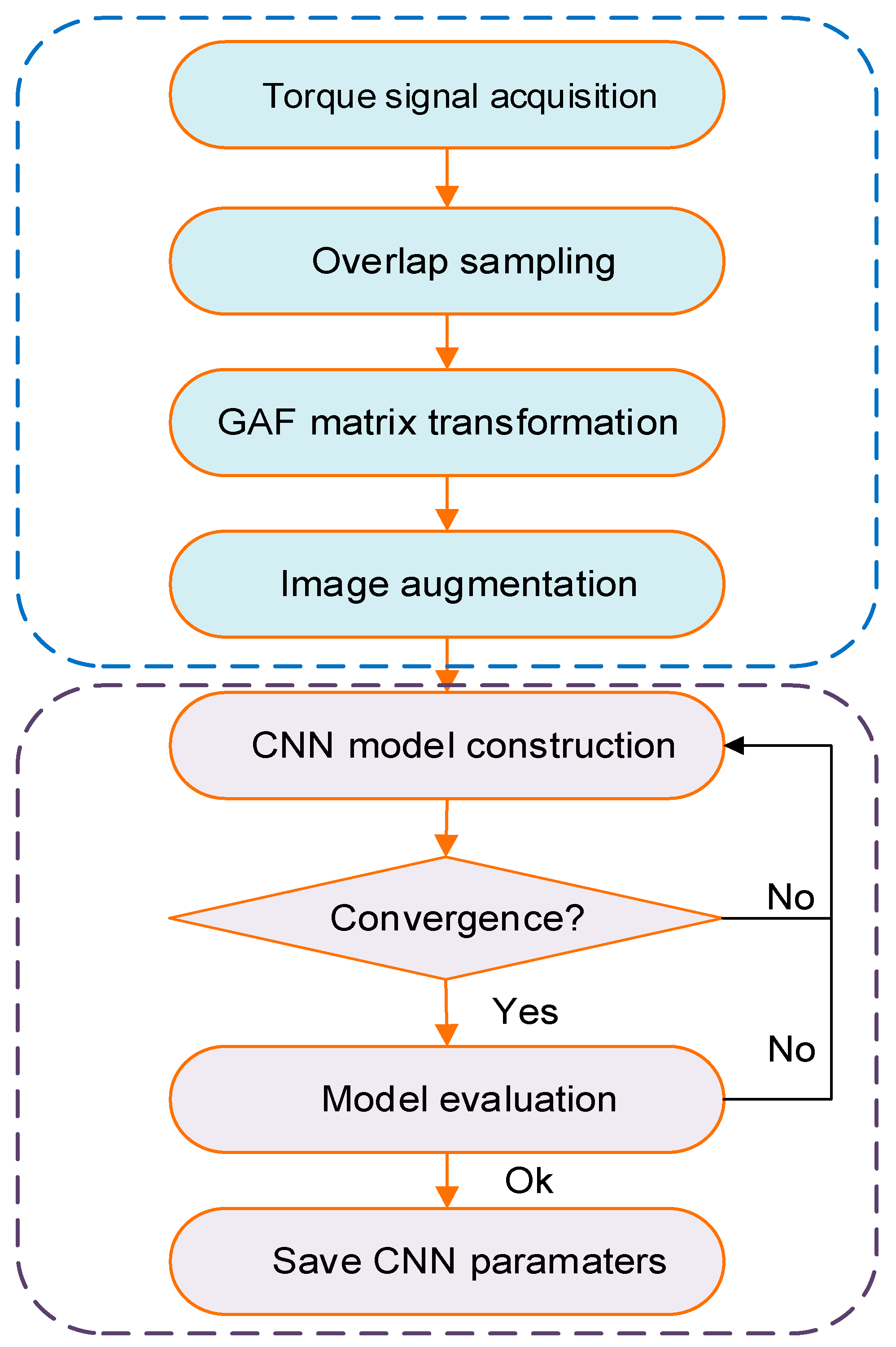
3. Image Transformation and Augmentation

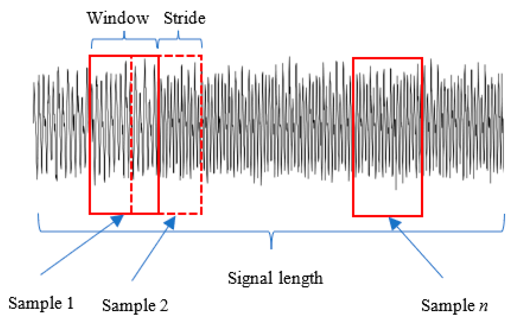
3.1. Image Transformation of the Torque Signal based on GAF

The GAF method is used to transform the original torque signal into two-dimensional images to reflect amplitude fluctuation and average change of torque. This transformation method can make good use of the advantages of CNN in image fault feature extraction. The encoding mapping of time series is unique with GAF, being able to completely preserve signal information and display the change between each numerical point. The transformation is completed based on polar coordinates and the Gramian matrix, and the process is as follows [37]:

The torque signal T = {T₁, T₂, T₃, …, T_n} is mapped to [−1, 1] using the Min−Max scaler, and the mapping process is expressed as

$${\tilde{T}}_j=\frac{\left[T_j-min(T)\right]+\left[T_j-max(T)\right]}{max(T)-min(T)},$$

(2)

Mapping the result of the Equation (1) to the polar coordinate system, the expression is obtained as follows:

$$\{\begin{array}{l}{\theta }_j=\arccos ({\tilde{T}}_j), -1\le {\tilde{T}}_j\le 1\\ r_j=t_j/N, t_j\in N\end{array}$$

(3)

where θ_j is the angle in polar coordinates; r_j is the radius, being the jth value after the normalization of the torque signal; t_j is the timestamp; and N is the total time. GFA defines the correlations between different points in time by adding or subtracting trigonometric functions, and the mapping of time series on polar coordinates is unique because of the monotonicity of the cosine function on [0, π].

GAF is divided into the Gram angle difference field (GADF) and the Gramian angular summation field (GASF). The GASF and GADF matrix expressions are shown in Formulas (3) and (4). It can be seen that the GASF matrix retains the time correlation of diagonal lines better than GADF. Hence, the GASF method was adopted to encode the torque signal.

$$\begin{array}{ll}{G}_{ASF}=& \left[\begin{array}{llll}\cos ({\theta }_1+{\theta }_1)& \cos ({\theta }_1+{\theta }_2)& \cdots & \cos ({\theta }_1+{\theta }_n)\\ \cos ({\theta }_2+{\theta }_1)& \cos ({\theta }_2+{\theta }_2)& \cdots & \cos ({\theta }_2+{\theta }_n)\\ ⋮& ⋮& & ⋮\\ \cos ({\theta }_n+{\theta }_1)& \cos ({\theta }_n+{\theta }_2)& \cdots & \cos ({\theta }_n+{\theta }_n)\end{array}\right]\\ \hfill =& {\tilde{T}}^{\prime }\cdot T-\sqrt{I-{\tilde{T}}^2{ }^{\prime }}\cdot \sqrt{I-{\tilde{T}}^2}\end{array}$$

(4)

$$\begin{array}{ll}{G}_{ADF}=& \left[\begin{array}{llll}sin({\theta }_1-{\theta }_1)& sin({\theta }_1-{\theta }_2)& \cdots & sin({\theta }_1-{\theta }_n)\\ sin({\theta }_2-{\theta }_1)& sin({\theta }_2-{\theta }_2)& \cdots & sin({\theta }_2-{\theta }_n)\\ ⋮& ⋮& & ⋮\\ sin({\theta }_n-{\theta }_1)& sin({\theta }_n-{\theta }_2)& \cdots & sin({\theta }_n-{\theta }_n)\end{array}\right]\\ \hfill =& \sqrt{I-{\tilde{T}}^2{ }^{\prime }}\cdot \tilde{T}-{\tilde{T}}^{\prime }\cdot \sqrt{I-{\tilde{T}}^2}\end{array}$$

(5)

where I is the identity matrix.

For the original time series signal of one-dimensional torque with length n, the size of the GASF matrix is n × n after transformation. Taking 200 sampling points as an example, the GASF coding process is illustrated in Figure 9. The heat map generated after image coding contains RGB three-channel information, which occupies a large storage space and will increase the complexity of calculation, thus affecting the calculation speed. Gray processing was performed on the heat map obtained from the fault feature signal to improve the calculation speed and accuracy, as presented in Figure 9c.

Figure 10 shows part of the gray images transformed from the torque signal under different demagnetization faults at the rated load. It can be seen from Figure 10a,b that the distribution of black and white texture was dispersed relatively, and the feature change was not obvious between healthy and UD. The reason may be the uniform fault degree was set at a low level, belonging to a slight fault. Nevertheless, the white texture fault feature was obvious in PD, as well as in MD. This may have been be caused by torque fluctuations due to unbalanced electromagnetic force.

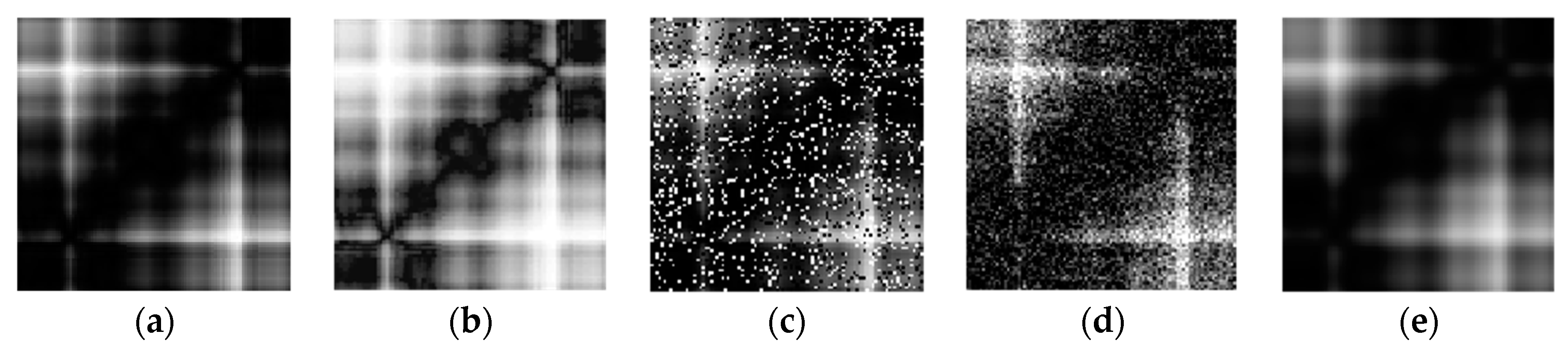
3.2. Image Augmentation

The low probability of demagnetization fault leads to the scarcity of fault data, which poses challenges in meeting the training data requirements for a deep learning network. Therefore, data augmentation is used to expand image datasets to improve the performance of CNN models. Image augmentation methods such as rotation, mirroring, and offset are not fully applicable due to the time sequence and periodicity of the one-dimensional fault signal, and thus this article achieved it through increasing image contrast, as well as adding noise and image blurring. The specific methods are as follows [38]:

3.2.1. Image Contrast Increasing

Image histogram statistics show the occurrence frequency of each gray level in the gray image. The equalization of the histogram can increase the dynamic range of gray values, make the distribution of gray levels balanced from 0 to 255, and improve the contrast intensity. The mapping is implemented through the cumulative distribution function as follows:

$$s_k=(L-1){\displaystyle \sum _{j=0}^k\frac{n_j}{MN}},k=0,1,2,\cdots ,L-1$$

(6)

where s_k is the new image, L is the number of gray levels in the original image, n_j is the number of current gray values in the original image, and MN is the total number of pixels in the original image. The gray mapping function converts the probability of the gray level of an original input image to the gray value of the output image.

3.2.2. Noise Increasing

Salt and pepper noise is caused by signal pulse intensity. The signal-to-noise ratio (SNR) is an indicator to measure noise, and its value belongs to [0, 1]. The disturbed pixel value will be changed to 255 or 0 after adding salt and pepper noise. Assuming the SNR is set to P, the mathematical expression of the salt and pepper noise is

$$N(w,h)=\{\begin{array}{l}I(w,h),r_1\ge P\\ 0,r_1<P,\mathrm{and} r_2\ge 0.5\\ 255,r_1<P,\mathrm{and} r_2<0.5\end{array}$$

(7)

where w = (w = 1, …, W) is the width of the image, h = (w = 1, …, H) is the height of the image, N(w,h) is the pixel value of the new image at the position (w,h), I(w,h) is the pixel value of the original image at the position (w,h), and r₁ and r₂ are the random numbers between [0, 1]. P is set to 0.2 for adding salt and pepper noise.

Gaussian noise refers to adding the noise of Gaussian distribution on the original pixel, and its mathematical expression is

$$G(w,h)=\frac{1}{\sqrt{2\pi {\sigma }^2}}{e}^{-{[I(w,h)-X]}^2/(2{\sigma }^2)}$$

(8)

where G(w,h) is the pixel value of the new image at the position (w,h), and X and σ are the mean and variance of the Gaussian distribution, respectively. In this article, X was set to 0.01, and σ was set to 0.03 for increasing Gaussian noise.

3.2.3. Noise Blurring

Gaussian blur is used for image denoising and edge smoothing, and it can be regarded as the convolution of the image and the Gaussian distribution function. In the blurring process, each pixel value is set to the average value of surrounding pixels. The center point is taken as the origin when calculating the average value, and the larger the blur radius, the stronger the blurring effect. The two-dimensional Gaussian function can be derived from the one-dimensional Gaussian function, and the blurred pixel value expression is as follows:

$$G_b(w,h)=I(w,h)\frac{1}{2\pi {\sigma }^2}{e}^{-(w^2+h^2)/(2{\sigma }^2)}$$

(9)

In the formula, G_b(w,h) is the pixel value after the image is blurred, and σ is set to 1 for the blur processing.

Taking Figure 10c as an example, one of the images of PD fault, the augmented images are shown in Figure 11. It shows that the above method can increase the demagnetization fault samples effectively.

4. Demagnetization Fault Recognition Based on CNN

CNN has been widely used in the image processing field recently because of its high extraction ability of abstract features. The structure of CNN is mainly composed of multiple convolution layers, activation function layers, pooling layers, and fully connected layers. The difference between CNN and general neural networks is the convolution operation between input images and convolution kernel in feature extract. The weights corresponding to the neurons using CNN are the same, reducing the number of training parameters. Taking into account that the convolution operation has insufficient ability to process nonlinear transformations, a nonlinear activation function was introduced to increase model expression ability. The output process of the convolution layer is expressed as follows:

$$x_j^l=f({\displaystyle \sum _{i\in M}{x}_i^{l-1}\ast k_{ij}^l}+b_j)$$

(10)

where $x_j^l$ is the jth output feature map of layer l, $x_i^{l-1}$ is the input feature map of layer l, $k_{ij}^l$ is the convolution kernel, b_j is the bias quantity, and f(·) is the nonlinear activation function. This method reduces the uncertainty and complexity caused by artificial feature extraction.

After the convolutional layer, the pooling layer reduces the feature dimension and avoids overfitting. There are various pooling methods, such as max pooling and mean pooling. The pooling operation reduces the space size without changing the depth of the model, declining the computational cost effectively [39]. The fully connected layer connects the weights of all neurons and is constantly updated during training. It is located at the tail of the network model, and the output results are classified through softmax. In this article, the gray images transformed from torque signal are taken as the network input, and the output is the demagnetization fault type.

4.1. Dataset Establishment

Overlap sampling was adopted to expand the number of fault samples. A sliding window was used to segment the torque signal into vectors of equal size and store them in the same array. The fault sampling process is presented in Figure 12. Window size and stride length were the key parameters of overlapping sampling, and the sampling window size was set to 100, with the stride length set to 20 in this study.

Considering the load changes of PMSM due to uneven geology in actual drilling, five load conditions were set for sampling. The sampling frequency was adopted at 7000 Hz, and the sampling time was about 1.8 s. The degree of demagnetization was set to 10% for UD, and 30% of the permanent magnet numbered N1 for PD. Moreover, only two different degrees of demagnetization were considered for MD in this study, setting the degree of demagnetization of numbered N1 to 30%, and 10% for the remaining PMs. All the acquired torque signals were transformed into gray images and performed enhancement operations on the images randomly. A total of 38,000 gray images were integrated into the dataset, and the four fault classification labels were set to 0, 1, 2, and 3, separately. It should be noted that the classification labels of demagnetization fault were independent of the running state of the PMSM. The information related to the PMSM in the dataset is shown in

Table 2. Details of the dataset.

Demagnetization Type and Degree	Number of Samples	Fault Label	Operating State
Healthy	9500	0	Speed: 300 rpm; Loads: 0, 1/4 TN, 1/2TN, 3/4TN, and TN.
UD (10%)	9500	1
PD (N1:30%)	9500	2
MD (N1:30% remaining PMs:10%)	9500	3

.

4.2. Structure of the Designed CNN

The CNN model was built based on MATLAB, which not only reduced the calculation time but also ensured the stable running of the program. An optimal network model was obtained by comparing different convolution layers and different convolution kernel sizes. The optimal CNN structure design is shown in Figure 13. The proposed CNN structure is illustrated in Figure 13. The feature extraction part consisted of three groups of convolution layers and pooling layers, and the size of input gray images was 100 × 100. The normalization method adopted global normalization after the convolution operation. ReLU was selected as an activation function that can improve the dynamics of the training process. To prevent the model from overfitting, a dropout layer was added in front of the fully connected layer. A total of 80% of the dataset was selected randomly for training, and the remaining 20% was used for verification during the training process. The number of outputs of the CNN neurons was equal to the number of fault categories.

The basic parameters of the established model are shown in

Table 3. Basic parameters of the established model of the CNN.

Name of the Parameter	Value
Number of convolution layers	3
Convolution kernel size for each layer	3 × 3
Number of convolution kernels per layer	20-40-40
Activation function	ReLU
Pooling method	Max
Pooling size	2 × 2
Probability of dropout layer	0.3

. The CNN training method adopted the stochastic gradient descent with the momentum (SGDM) method, with a momentum coefficient equal to 0.9. Momentum accumulates the average of the previous gradient of mini-batch randomly generated in the training dataset for accelerated learning. The training was carried out with an initial learning rate equal to 0.001, and the number of epochs was set to 20 with a total number of 2380 iterations.

4.3. Analysis of the Classification Results and Visualization of Features

The training process of the proposed network is presented in Figure 14, and it can be seen that the approximate accuracy of demagnetization recognition was equal to 98.33%. Moreover, the error function had high accuracy and stability during the training process.

Figure 15 presents the feature maps (FMs) obtained after the convolution operation of different demagnetization faults. A total of 20 FMs were output in the first convolution layer and were merged into 5 × 4 rectangular block graphs, as shown in Figure 15a. A total of 40 FMs were output in the second and third convolution layers, which were merged into 5 × 8 rectangular block graphs, respectively, as shown in Figure 15b,c. It can be seen that with the increase in convolutional layers, white texture features were increased, and the black texture areas were decreased in each demagnetization fault. In the same convolutional layer, the gray FMs with demagnetization faults had a larger white texture area than the healthy state. From the perspective of partial and MD, white texture is also related to the degree of demagnetization Accordingly, the training CNN model is most likely to use white texture as a symptom feature to recognize fault types.

5. Experimental Verification

5.1. Experimental Platform Establishment

To verify the effectiveness of the proposed fault diagnosis method, an experimental platform was established as shown in Figure 16. It consists of faulty motor, magnetic powder brake, torque and speed sensor, data acquisition instrument, and industrial computer. Three types of demagnetization were set according to Table 2. The PMs with different demagnetization degrees were obtained by heating them at different temperatures according to the thermal demagnetization model. We found that 10% and 30% demagnetization degrees can be obtained at 170 °C and 200 °C, respectively. One section of the drilling PMSM was selected for the fault experiment, considering the manufacturing cost. An FZ200J/Y magnetic powder brake was adopted to provide loads to the test motor, with a maximum load of 200 N·m. The torque and speed sensor was used to measure output torque with a type of ZJ-A, and the torque signal data were stored and read by the torque and speed power acquisition instrument of TR-3. A Windows 64-bit industrial computer configured with an Intel(R) Core(TM) i7-11700F 2.50 GHz processor was used for data processing and CNN training.

The loads changed from 0-T_N with an interval of 0.3T_N under different demagnetization fault conditions during the experiment. The acquired torque signals were converted into a total of 8480 gray images, and each demagnetization type contained 2120 gray images.

5.2. Model Evaluation with the Experimental Data

The experimental data were used as the testing dataset to assess the proposed CNN model, and the CNN model performance was evaluated in the form of a confusion matrix. The confusion matrix is a common method for evaluating multiple classification tasks, including accuracy, precision, recall rate, and k coefficient, which are expressed as follows:

$$AR=\frac{TP+TN}{TP+TN+FP+FN}$$

(11)

$$PR=\frac{TP}{TP+FP}$$

(12)

$$RCR=\frac{TP}{TP+FN}$$

(13)

$$k=\frac{p_c-p_e}{1-p_e}$$

(14)

where AR is the accuracy of the model, TP is true positive, FP is false positive, TN is true negative, FN is false negative, PR is the precision of recognition, RCR is the recall rate of recognition, k is Cohen’s coefficient, Pc is the proportion of observed agreement and Pe is the proportion of randomly generated agreement, and k is used to measure the accuracy of a classifier. Figure 17 shows the confusion matrix for the testing dataset. It can be seen clearly that the overall accuracy of fault detection reached 97.41%, which was lower than verification accuracy. The reason was that the finite element simulation assumes the PMSM as an ideal state, but it may be affected by electromagnetic interference, mechanical friction, and other factors in the experiment. Since the testing dataset contains gray images transformed from torque signals under different loads, it indicates the diagnosis method proposed in this article is immune to changes in loads. The recognition effectiveness of UD fault reached 98.92%. About 1.08% of the true positive samples were misclassified as healthy, with the reason potentially being that the fault degree of UD was set relatively small, and the compensation would be produced by the controller after demagnetization, such as increasing the stator current, resulting in the misjudgment of these two faults. The recognition of MD faults is the most difficult, because of the little changes in output torque signal compared to PD, as the gray fault map features are highly similar, leading to an increase in error classification. Cohen’s coefficient was calculated to be 0.96 with a high homogeneity by different evaluators, indicating the proposed fault recognition model has good classification ability.

6. Discussion and Conclusions

A demagnetization fault intelligent diagnosis method using image transformation (GAF) and CNN image recognition is proposed in this article. Finite element simulation and an experiment were used to verify and test the proposed method. The results show that this method can effectively recognize various demagnetizations of PMSM used in electric drilling tools, which provides a good solution to the problem that traditional fault diagnosis methods cannot detect multiple demagnetization faults at the same time. It also provides a new strategy for fault maintenance. GAF coding preserves the uniqueness of torque signal effectively in time and combines it with the good symptom extraction ability of CNN to ensure high-precision fault detection in a steady state and transient state. In addition, the diagnostic method is not affected by the demagnetization degree and working condition of PMSM. The conclusions are summarized as follows:

(1)

The output torque signal of a PMSM can be used as an effective means of gaining information on a demagnetization fault. The GASF matrix transformation makes fault feature extraction easier.

(2)

Transforming the one-dimensional torque signal into gray images for demagnetization fault diagnosis requires less data than processing data directly, reduces the computer storage space, and improves the calculation rate effectively at the same time.

(3)

Compared with PD and MD, the proposed method has higher diagnostic accuracy for UD with torque signal.

(4)

The proposed demagnetization recognition method is immune to the loads, which makes full use of the advantages of CNN image recognition, and the designed deep network model has good stability and robustness.

Future work includes the further study of image-converting technology for one-dimensional signals and the diagnosis of the degree of demagnetization faults.

References

1. Du, Y.; Wu, L.; Zhan, H.; Ruan, G.; Fang, Y. Investigation of post demagnetization unbalanced magnetic force in PM machines considering short circuit faults. IEEE Trans. Transp. Electrif. 2021, 7, 2728–2742. [Google Scholar] [CrossRef]
2. Prieto, M.D.; Espinosa, A.G.; Ruiz, J.R.R.; Urresty, J.C.; Ortega, J.A. Feature extraction of demagnetization faults in permanent-magnet synchronous motors based on box-counting fractal dimension. IEEE Trans. Ind. Electron. 2011, 58, 1594–1605. [Google Scholar] [CrossRef]
3. Liu, Z.; Xiao, W.; Cui, J.; Mei, L. Application of an information fusion method to the incipient fault diagnosis of the drilling permanent magnet synchronous motor. J. Pet. Sci. Eng. 2022, 219, 111124. [Google Scholar] [CrossRef]
4. Zhu, M.; Yang, B.; Hu, W.; Feng, G.; Kar, N.C. Vold-Kalman filtering order tracking based rotor demagnetization detection in PMSM. IEEE Trans. Ind. Appl. 2020, 55, 5768–5778. [Google Scholar] [CrossRef]
5. Song, J.; Zhao, J.; Dong, F.; Zhao, J.; Song, X. Demagnetization fault detection for double-sided permanent magnet linear motor based on three-line magnetic signal signature analysis. IEEE/ASME Trans. Mechatron. 2020, 25, 2815–2827. [Google Scholar] [CrossRef]
6. Zhu, M.; Hu, W.; Kar, N.C. Acoustic noise-based uniform permanent-magnet demagnetization detection in SPMSM for high-performance PMSM drive. IEEE Trans. Transp. Electrif. 2018, 4, 303–313. [Google Scholar] [CrossRef]
7. Gritli, Y.; Rossi, C.; Casadei, D.; Zarri, L.; Filippetti, F. Demagnetizations diagnosis for permanent magnet synchronous motors based on advanced wavelet analysis. In Proceedings of the 20th International Conference on Electrical Machines (ICEM), Marseille, France, 2–5 September 2012. [Google Scholar]
8. Moosavi, S.S.; Djerdir, A.; Amirat, Y.A.; Khaburi, D.A. Demagnetization fault diagnosis in permanent magnet synchronous motors:A review of the state-of-the-art. J. Magn. Magn. Mater. 2015, 391, 203–212. [Google Scholar] [CrossRef]
9. Faiz, J.; Mazaheri-Tehrani, E. Demagnetization modeling and fault diagnosing techniques in permanent magnet machines under stationary and nonstationary conditions: An overview. IEEE Trans. Ind. Appl. 2017, 53, 2772–2785. [Google Scholar] [CrossRef]
10. Candelo-Zuluaga, C.; Riba, J.R.; Thangamuthu, D.V.; Garcia, A. Detection of partial demagnetization faults in five-phase permanent magnet assisted synchronous reluctance machines. Energies 2020, 13, 3496. [Google Scholar] [CrossRef]
11. Huang, F.; Zhang, X.; Qin, G.; Xie, J.; Peng, J.; Huang, S.; Long, Z.; Tang, Y. Demagnetization Fault Diagnosis of Permanent Magnet Synchronous Motors Using Magnetic Leakage Signals. IEEE Trans. Ind. Inf. 2023, 19, 6105–6116. [Google Scholar] [CrossRef]
12. Ruiz, J.R.R.; Rosero, J.A.; Espinosa, A.G.; Romeral, L. Detection of demagnetization faults in permanent-magnet synchronous motors under nonstationary conditions. IEEE Trans. Magn. 2009, 45, 2961–2969. [Google Scholar] [CrossRef]
13. Guo, X.; Chen, L.; Shen, C. Hierarchical adaptive deep convolution neural network and its application to bearing fault diagnosis. Measurement 2016, 93, 490–502. [Google Scholar] [CrossRef]
14. Park, Y.; Fernandez, D.; Lee, S.B.; Hyun, D.; Jeong, M.; Kommuri, S.K.; Cho, C.; Reigosa, D.D.; Briz, F. Online detection of rotor eccentricity and demagnetization faults in PMSMs based on Hall-effect field sensor measurements. IEEE Trans. Ind. Appl. 2019, 55, 2499–2509. [Google Scholar] [CrossRef]
15. Song, J.; Zhao, J.; Dong, F.; Zhao, J.; Xu, L.; Yao, Z. A new demagnetization fault recognition and classification method for DPMSLM. IEEE Trans. Ind. Inf. 2020, 16, 1559–1570. [Google Scholar] [CrossRef]
16. Xia, M.; Li, T.; Xu, L.; Liu, L.; de Silva, C.W. Fault diagnosis for rotating machinery using multiple sensors and convolutional neural networks. IEEE/ASME Trans Mechatron. 2018, 23, 101–110. [Google Scholar] [CrossRef]
17. Jiang, G.; He, H.; Yan, J.; Xie, P. Multiscale convolutional neural networks for fault diagnosis of wind turbine gearbox. IEEE Trans. Ind. Electron. 2019, 66, 3196–3207. [Google Scholar] [CrossRef]
18. Liu, W.; Ma, T.; Xie, Q.; Tao, D.; Cheng, J. LMAE: A large margin auto-encoders for classification. signal processing. Signal Process 2017, 141, 137–143. [Google Scholar] [CrossRef]
19. Tran, V.T.; Althobiani, F.; Ball, A. An approach to fault diagnosis of reciprocating compressor valves using Teager-Kaiser energy operator and deep belief net-works. Expert Syst. Appl. 2014, 41, 4113–4122. [Google Scholar] [CrossRef]
20. Mandal, S.; Santhi, B.; Sridha, S.; Vinolia, K.; Swaminathan, P. Nuclear power plant thermocouple sensor-Fault detection and classification using deep learning and generalized likelihood ratio test. IEEE Trans. Nucl. Sci. 2017, 64, 1526–1534. [Google Scholar] [CrossRef]
21. Cho, H.C.; Knowles, J.; Fadali, M.S.; Lee, K.S. Fault detection and isolation of induction motors using recurrent neural networks and dynamic bayesian. IEEE Trans. Control Syst. Technol. 2010, 18, 430–437. [Google Scholar] [CrossRef]
22. Sun, W.; Zhao, R.; Yan, R.; Shao, S.; Chen, X. Convolutional discriminative feature learning for induction motor fault diagnosis. IEEE Trans. Ind. Inf. 2017, 13, 1350–1359. [Google Scholar] [CrossRef]
23. Skowron, M.; Orlowska-Kowalska, T.; Kowalski, C.T. Detection of Permanent Magnet Damage of PMSM Drive Based on Direct Analysis of the Stator Phase Currents Using Convolutional Neural Network. IEEE Trans. Ind. Electron. 2022, 69, 13665–13675. [Google Scholar] [CrossRef]
24. Faiz, J.; Nejadi-Koti, H. Demagnetization fault indexes in permanent magnet synchronous motors-an overview. IEEE Trans. Magn. 2016, 52, 8201511. [Google Scholar] [CrossRef]
25. Kao, I.H.; Wang, W.J.; Lai, Y.H.; Perng, J.W. Analysis of permanent magnet synchronous motor fault diagnosis based on learning. IEEE Trans. Instrum. Meas. 2019, 68, 310–324. [Google Scholar] [CrossRef]
26. Van, T.D.; Ui-Pil, C. Signal model-based fault detection and diagnosis for induction motors using features of vibration signal in two-dimension domain. J. Mech. Eng. 2011, 57, 655–666. [Google Scholar]
27. Uddin, J.; Islam, M.R.; Kim, J.M.; Kim, C.H. A two-dimensional fault diagnosis model of induction motors using a Gabor filter on segmented images. Int. J. Control Autom. 2016, 9, 11–22. [Google Scholar] [CrossRef]
28. Borecki, M.; Rychlik, A.; Vrublevskyi, O.; Olejnik, A.; Korwin-Pawlowski, M.L. Method of Non-Invasive determination of wheel rim technical condition using vibration measurement and artificial neural network. Measurement 2021, 185, 110050. [Google Scholar] [CrossRef]
29. Sun, Z.; Machlev, R.; Wang, Q.; Belikov, J.; Levron, Y.; Baimel, D. A public data-set for synchronous motor electrical faults diagnosis with CNN and LSTM reference classifiers. Energy AI 2023, 14, 100274. [Google Scholar] [CrossRef]
30. Kaya, Y.; Kuncan, M.; Kaplan, K.; Minaz, M.R.; Ertunc, H.M. A new feature extraction approach based on one dimensional gray level co-occurrence matrices for bearing fault classification. J. Exp. Theor. Artif. Intell. 2021, 33, 161–178. [Google Scholar] [CrossRef]
31. Li, Z.; Wu, Q.; Yang, S.; Chen, X. Diagnosis of rotor demagnetization and eccentricity faults for IPMSM based on deep CNN and image recognition. Complex Intell. Syst. 2022, 8, 5469–5488. [Google Scholar] [CrossRef]
32. Lin, L.; Wang, D.; Zhao, S.; Chen, L.; Huang, N. Power quality disturbance feature selection and pattern recognition based on image enhancement techniques. IEEE Access 2019, 7, 67889–67904. [Google Scholar] [CrossRef]
33. Liang, H.; Cao, J.; Zhao, X. Average descent rate singular value decomposition and two-dimensional residual neural network for fault diagnosis of rotating machinery. IEEE Trans. Instrum. Meas. 2022, 71, 3512616. [Google Scholar] [CrossRef]
34. Gritli, Y.; Tani, A.; Rossi, C.; Casadei, D. Assessment of current and voltage signature analysis for the diagnosis of rotor magnet demagnetization in five-phase AC permanent magnet generator drives. Math. Comput. Simul. 2019, 158, 91–106. [Google Scholar] [CrossRef]
35. Chakraborty, S.; Keller, E.; Ray, A.; Mayer, J. Detection and estimation of demagnetization faults in permanent magnet synchronous motors. Electr. Power Syst. Res. 2013, 96, 225–236. [Google Scholar] [CrossRef]
36. Huang, G.; Li, J.; Fukushima, E.F.; Zhang, C.; He, J.; Zhao, K. An improved equivalent-input-disturbance approach for PMSM drive with demagnetization fault. ISA Trans. 2020, 105, 120–128. [Google Scholar] [CrossRef]
37. Gao, W.; Jin, H.; Yang, G. Series arc fault diagnosis method of photovoltaic arrays based on GASF and improved DCGAN. Adv. Eng. Inf. 2022, 54, 101809. [Google Scholar] [CrossRef]
38. Shorten, C.; Khoshgoftaar, T.M. A survey on image data augmentation for deep learning. J. Big Data 2019, 6, 60. [Google Scholar] [CrossRef]
39. Gu, J.; Wang, Z.; Kuen, J.; Ma, L.; Shahroudy, A.; Shuai, B. Recent advances in convolutional neural networks. Pattern Recognit. 2018, 77, 354–377. [Google Scholar] [CrossRef]
Figure 1. The proposed demagnetization fault diagnosis process.
Electronics 13 00189 g001
Figure 2. Magnetization and demagnetization processes of PM. (a) B-H curve of the PM; (b) demagnetization curve of the PM.
Electronics 13 00189 g002
Figure 3. Thermal demagnetization test platform of the PMs.
Electronics 13 00189 g003
Figure 4. The regression curves with three modeling methods. (a) The regression curve of temperature–magnetic flux. (b) The regression curve of temperature–demagnetization degree.
Electronics 13 00189 g004aElectronics 13 00189 g004b
Figure 5. The PMSM model for electric drilling tools. (a) Physical PMSM. (b) FEM of the PMSM and PM number.
Electronics 13 00189 g005
Figure 6. The output torque of the PMSM in healthy and demagnetization states.
Electronics 13 00189 g006
Figure 7. The BEMF of the PMSM in healthy and demagnetization states.
Electronics 13 00189 g007
Figure 8. The air gap flux density BL in healthy and demagnetization states.
Electronics 13 00189 g008
Figure 9. Coding process of GASF. (a) Sampling. (b) Polar coordinate mapping. (c) Image coding.
Electronics 13 00189 g009
Figure 10. Images transformed from the output torque signal. (a) Healthy state. (b) UD state. (c) PD state. (d) MD state.
Electronics 13 00189 g010
Figure 11. Images transformed from the output torque signal. (a) Original image. (b) Equalization histogram image. (c) Salt and pepper noise. (d) Gaussian noise. (e) Gaussian blur.
Electronics 13 00189 g011
Figure 12. Fault sampling process.
Electronics 13 00189 g012
Figure 13. The proposed CNN model structure.
Electronics 13 00189 g013
Figure 14. Training process of the CNN.
Electronics 13 00189 g014
Figure 15. FMs in each convolution layer. (a) FMs in the first convolution layer. (b) FMs in the second convolution layer. (c) FMs in the third convolution layer.
Electronics 13 00189 g015
Figure 16. Experimental device. (a) Demagnetization rotor of the prototype. (b) Magnetic powder brake and torque and speed sensor. (c) Data acquisition instrument. (d) Industrial computer.
Electronics 13 00189 g016
Figure 17. Confusion matrix for the testing dataset.
Electronics 13 00189 g017