Article

An Improved Method for Photovoltaic Forecasting Model Training Based on Similarity

1
School of Advanced Interdisciplinary Studies, Hunan University of Technology and Business, Changsha 410205, China
2
Xiangjiang Laboratory, Changsha 410205, China
*
Author to whom correspondence should be addressed.
Electronics 2023, 12(9), 2119; https://doi.org/10.3390/electronics12092119
Submission received: 28 March 2023 / Revised: 16 April 2023 / Accepted: 19 April 2023 / Published: 6 May 2023
(This article belongs to the Special Issue Advances in Image Processing and Detection)

Abstract

:
Photovoltaic (PV) power generation is the most widely adopted renewable energy source. However, its inherent unpredictability poses considerable challenges to the management of power grids. To address the arduous and time-consuming training process of PV prediction models, which has been a major focus of prior research, an improved approach for PV prediction based on neighboring days is proposed in this study. This approach is specifically designed to handle the preprocessing of training datasets by leveraging the results of a similarity analysis of PV power generation. Experimental results demonstrate that this method can significantly reduce the training time of models without sacrificing prediction accuracy, and can be effectively applied in both ensemble and deep learning approaches.

1. Introduction

Following the outbreak of the COVID-19 pandemic, social development in all countries has been greatly hampered. The energy crisis has become very urgent, while the slowdown in economic development caused by the pandemic has not yet been resolved. Due to the non-renewable nature of fossil energy, the disadvantages of power generation methods that rely on the consumption of fossil energy have become very acute. In the UK and EU, the price of electricity has risen rapidly due to the lack of fossil energy reserves, and Northeast China has issued a notice of power restriction. As fossil energy represents a pollution issue for the environment [1], countries around the world have formulated policies on carbon emission control. China has put forward a goal of reaching peak carbon emissions by 2030 and carbon neutrality by 2060, which is referred to as the double carbon target.
To replace fossil energy, it is necessary to vigorously develop renewable energy sources. Solar energy, as the renewable energy form with the widest range of application and the lowest threshold, is developing very rapidly. However, both power aggregators and countries have to maintain a balance between supply and demand with respect to electricity, and the biggest drawback of photovoltaic power generation is its uncertainty, which makes it difficult to achieve accurate control of power levels [2]. As a result, the accurate prediction of photovoltaic power generation is of great importance.
The rapid advancement of deep learning has garnered widespread attention among scholars due to its exceptional learning and adaptability capabilities [3,4]. As a result, several deep learning-based techniques have been developed for photovoltaic power generation prediction. Artificial Neural Networks (ANN) are one commonly used approach [5,6,7,8,9,10]; they often employ statistical analysis or sensitivity analysis to select input variables or are used to combine deep learning with other methods [11,12] such as pattern extraction, bootstrapping, etc. These studies have significantly improved the accuracy of photovoltaic power generation prediction by targeting input variables, model optimization, and model combination. Long Short-Term Memory (LSTM) networks, which are well-suited for handling problems with multiple variables, have emerged as a popular choice for time series prediction problems. Most researchers employ LSTM as a foundation and then integrate multiple models to enhance the prediction process [13,14,15,16,17].
Most of the research on PV generation forecasting uses machine learning models such as Random Forests (RF), Support Vector Machines (SVM), and Deep Learning via Long Short-Term Memory (LSTM), as well as other learning methods using a combination of prediction models. Improvements to the accuracy of forecasting are based on the analysis of data patterns in PV power generation or on targeted improvements to the model, such as seasonality. Alternatively, a combination of different models can be used. The state of the weather has an extremely important impact on the efficiency of solar power production, mainly solar irradiance and temperature [18], and as such can be divided into two main categories based on weather conditions: direct prediction methods for PV power generation [19,20,21,22,23,24,25,26,27,28], and indirect prediction methods that predict the solar irradiance in order to derive PV power generation. Datasets for solar energy forecasting mainly consist of time series, as weather conditions are strongly correlated with time [19].
Based on the existing research, an experimental analysis of the similarity and repeatability of PV generation is conducted in this paper to quantify its characteristics. Then, a new method of extracting the dataset of adjacent days is proposed based on this analysis. Furthermore, the time range of adjacent days is specified in order to optimize the training dataset, thereby reducing the model training time. The contributions of this paper are as follows:
  • The regularity of PV power generation is explored through data processing and experimental analysis, finding extremely high similarity in historical power generation data and determining the key influence of solar irradiance.
  • Through experimental analysis of the number of neighboring days, the optimal number of neighboring days for PV power generation prediction is found. It is possible to achieve improved prediction accuracy compared to using the full dataset for training. In addition, the proposed approach is able to find the smallest possible dataset size for training.
  • Based on the existing research, along with integrating the above experimental analysis results, it is demonstrated experimentally that the proposed method for improved PV power generation prediction has a significantly improved effect on training speed for deep learning, integration learning, etc., while keeping the prediction accuracy of PV power generation almost unchanged.
The rest of this paper is organized as follows: Section 2 specifies the existing methodological studies and the methodological framework of this paper. Similarity analysis experiments on PV generation are conducted in Section 3 to derive the method of extracting the dataset of adjacent day and experiments are conducted to find the threshold for determining adjacent days. Section 4 applies the proposed method of this paper with models such as random forest to validate its effectiveness and generalizability through experimental evaluation. Finally, Section 5 draws conclusions and provides the method’s future outlook.

2. Related Works

According to the above introduction, the direct prediction method mostly classifies the weather. The weather factors are extracted by dimensional analysis. Then, the dimensions with high impact are obtained as model inputs [20]. Gao M classified the weather for PV data into ideal weather (sunny days) and non-ideal weather (rainy or snowy days), then applied different prediction methods for both types of weather [21]. Binghui Li performed weather-informed estimation of ramping needs in electricity markets and captured influences by principal component analysis of weather to quantify weather conditions [22]. To consider the correlation between different explanatory weather variables, Mucun Sun used the Copula to model the multivariate joint distribution between predicted and observed weather variables [23]. For cases with incomplete data or lack of data, Laura S and Qiaoqiao Li provided methods based on sunny day index calculation and recursive LSTM prediction for interpolation, with significant effectiveness in practical scenarios [24,25].
To address the problem of the large datasets required for PV prediction, Haoran Wen used federal learning to aggregate historical PV data from various locations using four training strategies with much higher prediction performance [26]. Huaizhi Wang adapted a neural network to provide a clear interpretation of the relationship between prediction model inputs and outputs for PV prediction [27]. Xiaoqiao Huang assembled several models for solar irradiance prediction using a combination of WPD, CNN, LSTM, and MLP, which outperformed the traditional baseline model [28]. Vahid Nourani obtained the dependence of time series on seasonality by establishing two seasonal LSTMs (SLSTM and WLSTM) [29]. Abdel Nasser used Choquet to simulate the correlation of inputs, then aggregated them and transported them to LSTM [30].
Addressing seasons and weather is critical to the diversity and flexibility of a VPP energy portfolio. Mainly, historical data are classified or solar irradiance is analyzed to narrow down the influence of weather on data performance [31,32,33,34,35,36,37,38]. Alternatively, the spatio-temporal characteristics of data can be analyzed and extracted [39,40,41]. Iraklis C amplified seasonal data to enhance possible instability of renewable energy production, then predicted the day-ahead flexibility provided by VPP in distributed energy systems [42]. Bandara K used MSTL and a multi-period time series decomposition algorithm to remove the effect of seasonality [43], and proposed a three-layer forecasting framework called LSTM-MSNet. Ghimire S used convolutional networks to extract data features for the predictor variables and LSTM for training and prediction, achieving high accuracy in short-term prediction and concluding that the prediction of solar radiation can be integrated into the grid to provide strategic support for supply of solar power [44]. Xiangfei Kong proposes a TCN attention-based time convolutional network model, which combines the advantages of TCN’s time series prediction to optimize the gradient problem during calculation and effectively improve prediction accuracy [45]. Moreover, several preprocessing techniques have been developed for weather classification [46,47,48,49], and their impact on prediction accuracy has been demonstrated through empirical studies.
Study of the similarity of historical data and the state of weather has been an important direction for PV forecasting. In 2016, a similarity approach for PV prediction was proposed by Alexandre Boilley et al. [50]. Their method seeks the most similar period in a historical irradiance database using the data characteristics of the sample, i.e., it calculates the Euclidean distance between two time periods. Then, it converts the resulting equation into a convolutional form, which is effective in improving the prediction accuracy. Gao M et al. classified the weather and processed it separately, then trained four separate models for each season [21]. Hakan Acikgoz used a fully integrated empirical modal decomposition method with adaptive noise to analyze time series data, completing the processing of the original data with data reconstruction, deep feature extraction, and feature selection before submitting the final data for prediction [51]. Amir Rafati introduced a univariate data-driven approach for ultra-short-term forecasting of high-dimensional photovoltaic power generation. This approach uses persistence models and machine learning algorithms such as SVR and RF to improve forecasting [52]. Da Liu, on the other hand, used principal component analysis and K-means to cluster PV data [53] and used a differential evolutionary gray wolf optimizer to optimize RF for modeling. After such steps, the historical time points with the most similar characteristics to the predicted time points can be obtained. In addition, there are have been many studies using PSO (Particle Swarm Optimization) and other methods to deal with prediction [54,55,56,57,58].

3. Materials and Methods

3.1. Dataset Introduction

The dataset used in this paper consists of PV power generation data from Germany during the 2015–2019 period. In this dataset, the dimension contains the actual power generation in Germany along with related weather information such as real-time temperature, direct solar irradiance, and indirect solar irradiance. For the similarity analysis experiment, the inputs were time, electrical capacity, and solar irradiance, and the analysis was performed using years of historical power generation data. Based on the results of the analysis, a modified proximity day method was used for forecasting, with the generation data of those days adjacent to the forecast day used as input. The time interval was one day.

3.2. Photovoltaic Power Generation Analysis

These processing methods do not provide quantitative characterization of the data features of PV generation. DTW (Dynamic Time Warping) can quantify the similarity of multiple time series data in a comparative manner. The gap between multiple series can be derived through multiple comparisons, which is calculated as shown in the following Equations (1) and (2). In this paper, DTW is used to conduct similarity analysis of PV power generation data for historical years to explore the regularity and repeatability of PV power generation.
D T W ( X , Y ) = min ϕ d ϕ ( X , Y )
The core of the DTW algorithm is to calculate the distance between points in two sequences, generally the Euclidean distance, in order to obtain the distance matrix d ( x , y ) = f ( x i , y j ) 0 , where x i and y j are represented as a point in two sequences. Then, the cumulative distance matrix is calculated through the distance matrix, and the loss matrix shows the corresponding relationships between points. The solution of the twisted path is represented as Φ ( k ) = ( Φ x ( k ) , while Φ y ( k ) ) represents a point in two sequences. In addition, Φ ( k ) is the correspondence between the points in two sequences, meaning that the cumulative distance between the two sequences can be calculated using the formula. Finally, the curve with the smallest cumulative distance is calculated by dynamic programming (DP) and other methods, and is the twist curve solved by DTW:
γ ( i , j ) = d x i , y j + min γ ( i 1 , j 1 ) + 2 d ( i , j ) , γ ( i , j 1 ) + d ( i , j ) , γ ( i 1 , j ) + d ( i , j )
where d ( i , j ) is represented by x i and y j , the distance between two points γ ( i , j ) is denoted by x i , and y j is the cumulative distance between two points.
In this paper, we performed DTW calculations on three years of historical German PV power generation data to obtain their mutual similarity, then calculated the Minkowski distance of the data for comparison. After calculating the similarity for DTW, we calculated the Minkowski distance of the data for comparison. The Minkowski distance measures the similarity of two sets of data from a numerical point of view. The Minkowski distance was used to perform similarity analysis of PV generation data for the historical years studied in this paper and to quantify the degree of similarity for each year after constructing the adjacent day dataset. The calculation is shown in Equation (3) below.
i = 1 n x i y i 1 p
By taking different values for p, different distance calculation methods can be used. The most commonly used distances for this distance are 1 and 2, representing the Manhattan distance and Euclidean distance, respectively. When the value of p approaches infinity, it can be expressed as the Chebyshev distance.
Based on the above operations, a similarity analysis of the historical data was obtained, on which we base the proposed data processing method using adjacent days. The model training process is improved by similarity analysis of the data. Finally, the performance is compared with the existing baseline model. The analytical processing framework of this paper is shown in Figure 1.
The prediction model steps are as follows:
Step 1: The PV power generation data are separated by year to obtain PV power generation data for each year. Then, the generation data for each year are standardized (in this article, through normalization using MinMaxScaler) to obtain the standardized data.
Step 2: A prediction target day random_day is randomly selected from the dataset. An expanded neighboring-day dataset is constructed based on the time dimension of the prediction target day. Next, the neighboring day dataset is improved using historical data on PV power generation according to the method used to extract the expanded neighboring day dataset.
Step 3: The expanded adjacent day dataset is input to the algorithmic model for training and the training time is recorded as train_time; in the present study, six different models were used.
Step 4: PV power generation data are predicted based on the training results for the target prediction day in order to obtain the prediction result.
Step 5: The prediction accuracy of the model is evaluated using evaluation metrics such as nRMSE to verify the effectiveness of the method in this paper.
In this paper, the historical data are scattered, as shown in Figure 2 and Figure 3, the annual solar power production power has a certain degree of similarity. The production of photovoltaic power and the trend of change is similar, and shows a slow incremental trend year by year.
However, this similarity needs to be further quantified to prove that PV generation is similar between years; thus, DTW is used for quantification. As the annual power generation increases year by year, the DTW calculation value increases year by year as well. The improvement of power generation technology has an impact; in this paper, we perform the DTW calculation for the weather factor. In order to speed up the calculation and make the calculated values more intuitive, we normalized the PV power generation data before performing the DTW calculation and used the Minkowski distance with different p-values as the distance calculation method; the calculation results are shown in the following Table 1 and Table 2.
The results show that distance calculations using both the Manhattan distance and Euclidean distance reflect the similarity of PV generation between years, i.e., there is little difference in DTW distance between years. This means that in the absence of strong weather conditions or unexpected events, PV production and trends are very similar from year to year. The variation of PV power production in a certain time frame within the same month and on neighboring dates in different years shows very little fluctuation.
In this paper, the time series of irradiance and electricity production are plotted and analyzed, and it is found that the trend and regularity of photovoltaic power generation are closely related to the solar irradiance. Similarly, experiments by Moreno G have shown that solar irradiance plays a pivotal role in PV power generation. According to the thermogram of time series uncertain variables (Figure 4), it can be observed that the seasonality of PV power generation and weather effects are caused by changes in solar irradiance, and as such have an impact on the production of PV power generation, which reflects its extreme similarity even more.
Based on the above analysis, in this paper we further investigate the time range of neighboring days to the improve PV power forecasting model using neighboring days. The next section explores the effect of neighboring days on PV power forecasting for further time specification of neighboring days.

3.3. Adjacent Day

To determine the optimal neighboring day time range r, multiple neighboring time ranges are selected in this paper, as shown in the following r values for each of the neighboring day-based predictions. The experiments were performed on a PC equipped with Windows 10 and using Pycharm 2020.1.5 (Python 3.8). Ten experiments with different prediction target days were performed for each r fetch, and the LSTM parameters were fixed for each experiment. The performance was evaluated using the R2 and nRMSE calculated from the prediction results by averaging the experimental results at each r fetch.
r = 2 , 3 , 5 , 7 , 9 , 11 , 14
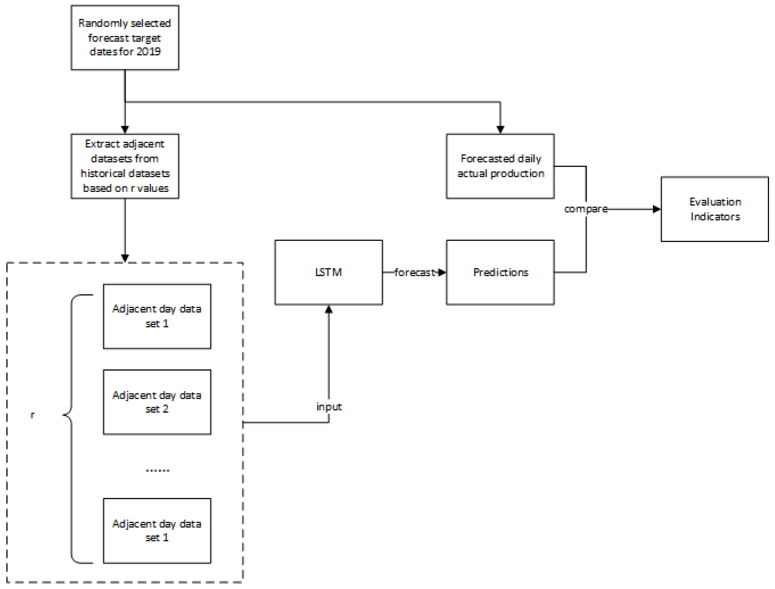
The flow of this experiment is shown in Figure 5. To maximize the acquisition of historical data, in this paper we chose a randomly selected date from the data for 2019 as the target prediction day. Based on the target prediction day, the data for adjacent days were obtained from the historical years to form the adjacent day dataset used as the input dataset for training. By setting different adjacent days, seven different adjacent day datasets were obtained, then these adjacent day datasets were used to train the prediction model, obtain the prediction results, and finally calculate the evaluation index of R2, nRMSE, and MAE. The experimental results obtained through this experimental process are shown in Table 3.
The experimental results show that the training set is too small if only the same-year neighboring days are used as the training set, which influences model training. In order to eliminate this effect, the dataset of adjacent days was expanded to include similar days, and the above experiments were conducted again using this expanded dataset as the training set. The results are shown in Table 4.
The adjacent day experiment reveals that the prediction accuracy can be significantly increased by appropriately increasing the number of adjacent days r. However, when the number of adjacent days is increased to seven days, the nRMSE and R2 values tend to level off, as shown in Figure 6; thus, the following judgments can be made:
  • An increase in the number of adjacent days results in a significant improvement in the accuracy of PV generation forecasting.
  • When the number of adjacent days is increased to seven days, the improvement in the accuracy of PV generation forecasting is very limited, with R2 and nRMSE values fluctuating around 0.992 and 11, respectively.
Through experimental validation analysis, the adjacent day and expanded adjacent day methods of improving the data (Method 1 and Method 2, respectively) are proposed in this paper:
Method 1: The set of adjacent dates for a target prediction day d p r e d within a time range r at the same time point in the same year are extracted and the set is denoted as D a . This set is used as the adjacent date dataset for d p r e d . The calculation method is as follows:
D a = d b e f o r e ,
c o n s t : b e f o r e r < b e f o r e < p r e d
where d p r e d denotes the proximate day of the forecast day, ‘pred’ denotes the time point of the forecast day, ‘before’ denotes those r time points less than the time point of the forecast day, and all the neighboring r adjacent days of the same year constitute the set of adjacent days D a , as shown in Figure 7.
To overcome the limitation of a small dataset, which can impact the training effect and prediction accuracy, we propose an improved method for extracting the adjacent day dataset based on the method of extracting the dataset of adjacent days and the similarity of historical data features, as shown in Method 2.
Method 2: Taking the year of the target prediction date d ( p r e d , y ) as the year, in each historical year before its year we take the set of historical-year adjacent days D h consisting of all time points in the time range centered on time point i of the same month and day of the target prediction date, with r as the radius, then sum up the above as D a to form the expanded set of adjacent days D k , as shown in Figure 8 and calculated as follows:
D k = D y + D a ,
D h = d h , i ,
c o n s t : p r e d > 0 , r > 0
p r e d r i p r e d + r , 0 < h < y
p r e d r j < p r e d

4. Experimental Evaluation

In order to evaluate the performance of this prediction model, in addition to the LSTM model used in the analysis experiments, Random Forest (RF), Convolutional Neural Network (CNN), and several other algorithms were chosen for comparison. The Keras neural network framework was used as the basis. Keras supports convolutional and recurrent networks and their combination, allowing for simple and fast prototyping. Sklearn is a machine learning library for python, which integrates classification, regression and clustering algorithms, including support vector machines, random forests and other algorithms. Sklearn was used to preprocess the data and implement support vector machines and other algorithms to compare their performance. Hyperparameter tuning was performed with the GridSearchCV grid search and cross-validation tool to find the most accurate parameters by continuous tuning and training the learner within the specified parameter range.
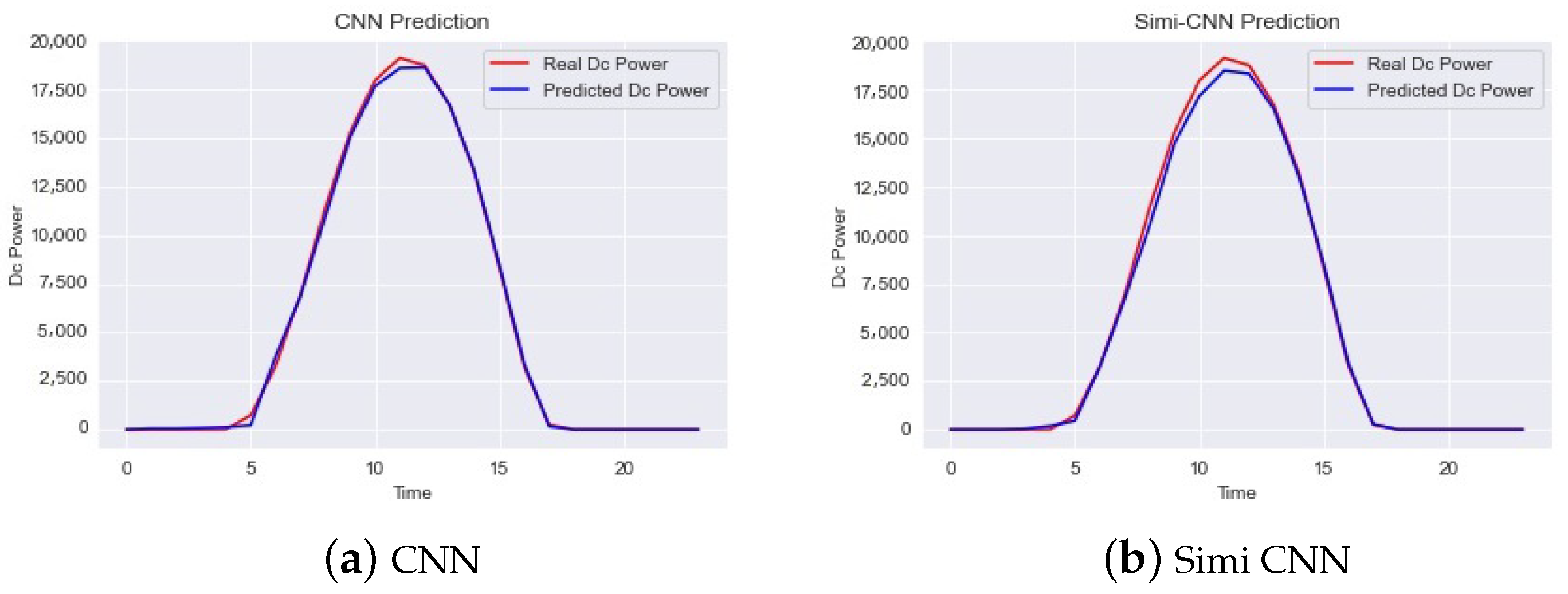
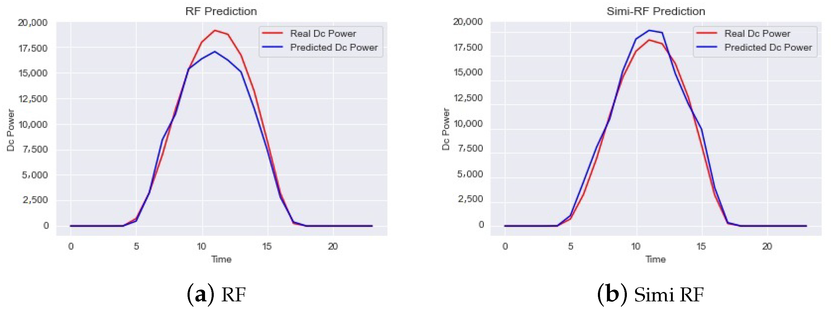
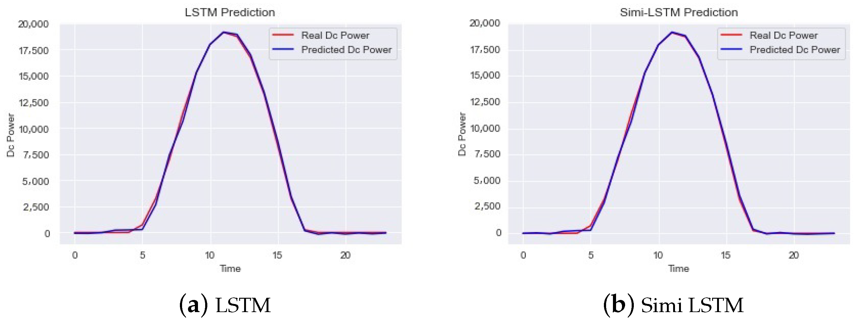
The experiments were run on a Windows 10 laptop with an i5 6300hq CPU and GTX 960M gpu. To compare the performance of the expanded adjacent days method, we evaluated it using RMSE and R2, taking the same input and output data formats (except for the amount of data) in order to keep the variables consistent. The input data were divided into two categories, one using the full dataset as the training set and one using only the expanded adjacent days dataset as the training set. The LSTM, CNN, and RF models using the improved training set with the expanded adjacency days proposed in this paper are referred to in the following as Simi-LSTM, Simi-CNN, and Simi-RF, and their prediction results are shown below (Figure 9, Figure 10 and Figure 11 and Table 5).
From Figure 9, Figure 10 and Figure 11, it can be seen that the improved model with the expanded adjacent days method provided in this paper predicts PV power generation with a fit no less than the original model. In addition, R2, MAE, and nRMSE remain smaller than the original model. Furthermore, this method effectively reduces the size of the required training dataset while achieving high prediction accuracy.
At the same time, the expanded adjacent days method provides a training speed advantage to the model. Therefore, the following conclusions can be drawn from our experimental results:
  • The expanded adjacent days model is effective in reducing the size of the dataset when performing PV generation forecasting, and the integrated learning method effectively reduces the training time for random forest models.
  • The improved model using expanded adjacent days is able to maintains a high level of accuracy in PV power prediction.

5. Conclusions

An improved method to reduce the size of the training dataset used in the training phase of PV power prediction models is provided in this paper. Based on the regularity and repeatability of photovoltaic power generation analyzed from historical data and the similarity of the photovoltaic power generation volume quantified for each year, the principle of using adjacent days to improve the training dataset is established.
Experimental results based on adjacent day analysis show that the proposed method can significantly improve training speed without sacrificing prediction accuracy compared to the original algorithms, demonstrating its universality. This means that researchers studying photovoltaic power generation can spend less time on model training. For best results the division of adjacent days should not be fixed, and models should be able to account for unexpected changes in weather conditions. These issues were not within the scope of the present paper. As a the next step, we intend to address the issue of changing weather conditions by dynamically adjusting the adjacent days based on the weather situation as a means of further improving the applicability and prediction accuracy of the proposed method.

Author Contributions

Conceptualization, L.L. and J.C.; methodology, L.L.; software, X.L.; validation, L.L., J.C. and J.Y.; formal analysis, X.L.; investigation, J.C.; resources, X.L.; data curation, J.Y.; writing—original draft preparation, L.L.; writing—review and editing, L.L.; supervision, X.L.; project administration, J.C.; funding acquisition, L.L. All authors have read and agreed to the published version of the manuscript.

Funding

This research was funded by the Major Project of National Natural Science Foundation of China, grant number 71991465, the National Key Research and Development Program of China, grant number 2021YFC3300603, and the Hunan Provincial Key Research Base in Philosophy and Social Science Smart Social and Big Data Intelligence Research Center.

Data Availability Statement

This review has no information related to it.

Acknowledgments

This research was supported by the Major Project of National Natural Science Foundation of China (Grant No. 71991465), the National Key Research and Development Program of China (Grant No. 2021YFC3300603), the Hunan Provincial Key Research Base in Philosophy and Social Science Smart Social and Big Data Intelligence Research Center.

Conflicts of Interest

The authors declare no conflict of interest.

References

  1. Kumari, P.; Toshniwal, D. Impact of lockdown on air quality over major cities across the globe during COVID-19 pandemic. Urban Clim. 2020, 34, 100719. [Google Scholar] [CrossRef]
  2. Espinar, B.; Aznarte, J.L.; Girard, R.; Moussa, A.M.; Kariniotakis, G. Photovoltaic Forecasting: A state of the art. In Proceedings of the 5th European PV-Hybrid and Mini-Grid Conference, Tarragona, Spain, 29–30 April 2010; OTTI-Ostbayerisches Technologie-Transfer-Institut: Regensburg, Germany, 2010; p. 250. [Google Scholar]
  3. Shi, H.; Xu, M.; Li, R. Deep learning for household load forecasting—A novel pooling deep RNN. IEEE Trans. Smart Grid 2017, 9, 5271–5280. [Google Scholar] [CrossRef]
  4. Kong, X.; Li, C.; Zheng, F.; Wang, C. Improved deep belief network for short-term load forecasting considering demand-side management. IEEE Trans. Power Syst. 2019, 35, 1531–1538. [Google Scholar] [CrossRef]
  5. Abuella, M.; Chowdhury, B. Solar power forecasting using artificial neural networks. In Proceedings of the 2015 North American Power Symposium (NAPS), Charlotte, NC, USA, 4–6 October 2015; IEEE: Piscataway, NJ, USA, 2015; pp. 1–5. [Google Scholar]
  6. Chen, C.; Duan, S.; Cai, T.; Liu, B. Online 24-h solar power forecasting based on weather type classification using artificial neural network. Sol. Energy 2011, 85, 2856–2870. [Google Scholar] [CrossRef]
  7. Almonacid, F.; Pérez-Higueras, P.; Fernández, E.F.; Hontoria, L. A methodology based on dynamic artificial neural network for short-term forecasting of the power output of a PV generator. Energy Convers. Manag. 2014, 85, 389–398. [Google Scholar] [CrossRef]
  8. Vaz, A.; Elsinga, B.; Van Sark, W.; Brito, M. An artificial neural network to assess the impact of neighbouring photovoltaic systems in power forecasting in Utrecht, the Netherlands. Renew. Energy 2016, 85, 631–641. [Google Scholar] [CrossRef]
  9. Sfetsos, A.; Coonick, A. Univariate and multivariate forecasting of hourly solar radiation with artificial intelligence techniques. Sol. Energy 2000, 68, 169–178. [Google Scholar] [CrossRef]
  10. Yona, A.; Senjyu, T.; Saber, A.Y.; Funabashi, T.; Sekine, H.; Kim, C. Application of neural network to one-day-ahead 24 h generating power forecasting for photovoltaic system, Intelligent Systems Applications to Power Systems. In Proceedings of the IEEE International Conference on Intelligent Systems Applications to Power Systems, Kaohsiung, Taiwan, 5–8 November 2007; pp. 1–6. [Google Scholar]
  11. Breinl, K.; Turkington, T.; Stowasser, M. Simulating daily precipitation and temperature: A weather generation framework for assessing hydrometeorological hazards. Meteorol. Appl. 2015, 22, 334–347. [Google Scholar] [CrossRef]
  12. Liu, B.; Nowotarski, J.; Hong, T.; Weron, R. Probabilistic load forecasting via quantile regression averaging on sister forecasts. IEEE Trans. Smart Grid 2015, 8, 730–737. [Google Scholar] [CrossRef]
  13. Liu, J.; Huang, X.; Li, Q.; Chen, Z.; Liu, G.; Tai, Y. Hourly stepwise forecasting for solar irradiance using integrated hybrid models CNN-LSTM-MLP combined with error correction and VMD. Energy Convers. Manag. 2023, 280, 116804. [Google Scholar] [CrossRef]
  14. Chang, Z.; Zhang, Y.; Chen, W. Electricity price prediction based on hybrid model of adam optimized LSTM neural network and wavelet transform. Energy 2019, 187, 115804. [Google Scholar] [CrossRef]
  15. Alizamir, M.; Shiri, J.; Fard, A.F.; Kim, S.; Gorgij, A.D.; Heddam, S.; Singh, V.P. Improving the accuracy of daily solar radiation prediction by climatic data using an efficient hybrid deep learning model: Long short-term memory (LSTM) network coupled with wavelet transform. Eng. Appl. Artif. Intell. 2023, 123, 106199. [Google Scholar] [CrossRef]
  16. Ghimire, S.; Deo, R.C.; Casillas-Pérez, D.; Salcedo-Sanz, S.; Sharma, E.; Ali, M. Deep learning CNN-LSTM-MLP hybrid fusion model for feature optimizations and daily solar radiation prediction. Measurement 2022, 202, 111759. [Google Scholar] [CrossRef]
  17. Jaihuni, M.; Basak, J.K.; Khan, F.; Okyere, F.G.; Sihalath, T.; Bhujel, A.; Park, J.; Lee, D.H.; Kim, H.T. A novel recurrent neural network approach in forecasting short term solar irradiance. ISA Trans. 2022, 121, 63–74. [Google Scholar] [CrossRef] [PubMed]
  18. Pazikadin, A.R.; Rifai, D.; Ali, K.; Malik, M.Z.; Abdalla, A.N.; Faraj, M.A. Solar irradiance measurement instrumentation and power solar generation forecasting based on Artificial Neural Networks (ANN): A review of five years research trend. Sci. Total Environ. 2020, 715, 136848. [Google Scholar] [CrossRef] [PubMed]
  19. Paulescu, M.; Brabec, M.; Boata, R.; Badescu, V. Structured, physically inspired (gray box) models versus black box modeling for forecasting the output power of photovoltaic plants. Energy 2017, 121, 792–802. [Google Scholar] [CrossRef]
  20. Sharadga, H.; Hajimirza, S.; Balog, R.S. Time series forecasting of solar power generation for large-scale photovoltaic plants. Renew. Energy 2020, 150, 797–807. [Google Scholar] [CrossRef]
  21. Gao, M.; Li, J.; Hong, F.; Long, D. Day-ahead power forecasting in a large-scale photovoltaic plant based on weather classification using LSTM. Energy 2019, 187, 115838. [Google Scholar] [CrossRef]
  22. Li, B.; Feng, C.; Siebenschuh, C.; Zhang, R.; Spyrou, E.; Krishnan, V.; Hobbs, B.F.; Zhang, J. Sizing ramping reserve using probabilistic solar forecasts: A data-driven method. Appl. Energy 2022, 313, 118812. [Google Scholar] [CrossRef]
  23. Sun, M.; Feng, C.; Zhang, J. Probabilistic solar power forecasting based on weather scenario generation. Appl. Energy 2020, 266, 114823. [Google Scholar] [CrossRef]
  24. Hoyos-Gómez, L.S.; Ruiz-Muñoz, J.F.; Ruiz-Mendoza, B.J. Short-term forecasting of global solar irradiance in tropical environments with incomplete data. Appl. Energy 2022, 307, 118192. [Google Scholar] [CrossRef]
  25. Li, Q.; Xu, Y.; Chew, B.S.H.; Ding, H.; Zhao, G. An integrated missing-data tolerant model for probabilistic PV power generation forecasting. IEEE Trans. Power Syst. 2022, 37, 4447–4459. [Google Scholar] [CrossRef]
  26. Wen, H.; Du, Y.; Lim, E.G.; Wen, H.; Yan, K.; Li, X.; Jiang, L. A solar forecasting framework based on federated learning and distributed computing. Build. Environ. 2022, 225, 109556. [Google Scholar] [CrossRef]
  27. Wang, H.; Cai, R.; Zhou, B.; Aziz, S.; Qin, B.; Voropai, N.; Gan, L.; Barakhtenko, E. Solar irradiance forecasting based on direct explainable neural network. Energy Convers. Manag. 2020, 226, 113487. [Google Scholar] [CrossRef]
  28. Huang, X.; Li, Q.; Tai, Y.; Chen, Z.; Zhang, J.; Shi, J.; Gao, B.; Liu, W. Hybrid deep neural model for hourly solar irradiance forecasting. Renew. Energy 2021, 171, 1041–1060. [Google Scholar] [CrossRef]
  29. Nourani, V.; Behfar, N. Multi-station runoff-sediment modeling using seasonal LSTM models. J. Hydrol. 2021, 601, 126672. [Google Scholar] [CrossRef]
  30. Abdel-Nasser, M.; Mahmoud, K.; Lehtonen, M. Reliable solar irradiance forecasting approach based on choquet integral and deep LSTMs. IEEE Trans. Ind. Inform. 2020, 17, 1873–1881. [Google Scholar] [CrossRef]
  31. Fouilloy, A.; Voyant, C.; Notton, G.; Motte, F.; Paoli, C.; Nivet, M.L.; Guillot, E.; Duchaud, J.L. Solar irradiation prediction with machine learning: Forecasting models selection method depending on weather variability. Energy 2018, 165, 620–629. [Google Scholar] [CrossRef]
  32. Michael, N.E.; Hasan, S.; Al-Durra, A.; Mishra, M. Short-term solar irradiance forecasting based on a novel Bayesian optimized deep Long Short-Term Memory neural network. Appl. Energy 2022, 324, 119727. [Google Scholar] [CrossRef]
  33. Lan, H.; Zhang, C.; Hong, Y.Y.; He, Y.; Wen, S. Day-ahead spatiotemporal solar irradiation forecasting using frequency-based hybrid principal component analysis and neural network. Appl. Energy 2019, 247, 389–402. [Google Scholar] [CrossRef]
  34. Prasad, R.; Ali, M.; Kwan, P.; Khan, H. Designing a multi-stage multivariate empirical mode decomposition coupled with ant colony optimization and random forest model to forecast monthly solar radiation. Appl. Energy 2019, 236, 778–792. [Google Scholar] [CrossRef]
  35. Kwon, Y.; Kwasinski, A.; Kwasinski, A. Solar irradiance forecast using naïve Bayes classifier based on publicly available weather forecasting variables. Energies 2019, 12, 1529. [Google Scholar] [CrossRef]
  36. Kushwaha, V.; Pindoriya, N.M. A SARIMA-RVFL hybrid model assisted by wavelet decomposition for very short-term solar PV power generation forecast. Renew. Energy 2019, 140, 124–139. [Google Scholar] [CrossRef]
  37. Qing, X.; Niu, Y. Hourly day-ahead solar irradiance prediction using weather forecasts by LSTM. Energy 2018, 148, 461–468. [Google Scholar] [CrossRef]
  38. Antonanzas-Torres, F.; Urraca, R.; Polo, J.; Perpiñán-Lamigueiro, O.; Escobar, R. Clear sky solar irradiance models: A review of seventy models. Renew. Sustain. Energy Rev. 2019, 107, 374–387. [Google Scholar] [CrossRef]
  39. Kumari, P.; Toshniwal, D. Long short term memory–convolutional neural network based deep hybrid approach for solar irradiance forecasting. Appl. Energy 2021, 295, 117061. [Google Scholar] [CrossRef]
  40. Lin, Y.; Koprinska, I.; Rana, M.; Troncoso, A. Pattern sequence neural network for solar power forecasting. In Proceedings of the Neural Information Processing: 26th International Conference, ICONIP 2019, Sydney, NSW, Australia, 12–15 December 2019; Proceedings, Part V 26. Springer: Berlin/Heidelberg, Germany, 2019; pp. 727–737. [Google Scholar]
  41. Jeon, H.J.; Choi, M.W.; Lee, O.J. Day-Ahead Hourly Solar Irradiance Forecasting Based on Multi-Attributed Spatio-Temporal Graph Convolutional Network. Sensors 2022, 22, 7179. [Google Scholar] [CrossRef]
  42. Iraklis, C.; Smend, J.; Almarzooqi, A.; Mnatsakanyan, A. Flexibility forecast and resource composition methodology for virtual power plants. In Proceedings of the 2021 International Conference on Electrical, Computer and Energy Technologies (ICECET), Cape Town, South Africa, 9–10 December 2021; IEEE: Piscataway, NJ, USA, 2021; pp. 1–7. [Google Scholar]
  43. Bandara, K.; Bergmeir, C.; Hewamalage, H. LSTM-MSNet: Leveraging forecasts on sets of related time series with multiple seasonal patterns. IEEE Trans. Neural Netw. Learn. Syst. 2020, 32, 1586–1599. [Google Scholar] [CrossRef]
  44. Ghimire, S.; Deo, R.C.; Raj, N.; Mi, J. Deep solar radiation forecasting with convolutional neural network and long short-term memory network algorithms. Appl. Energy 2019, 253, 113541. [Google Scholar] [CrossRef]
  45. Kong, X.; Du, X.; Xu, Z.; Xue, G. Predicting solar radiation for space heating with thermal storage system based on temporal convolutional network-attention model. Appl. Therm. Eng. 2023, 219, 119574. [Google Scholar] [CrossRef]
  46. Shi, J.; Lee, W.J.; Liu, Y.; Yang, Y.; Wang, P. Forecasting power output of photovoltaic systems based on weather classification and support vector machines. IEEE Trans. Ind. Appl. 2012, 48, 1064–1069. [Google Scholar] [CrossRef]
  47. Jiang, H.; Hong, L. Application of BP neural network to short-term-ahead generating power forecasting for PV system. Adv. Mater. Res. 2013, 608, 128–131. [Google Scholar] [CrossRef]
  48. Mellit, A.; Sağlam, S.; Kalogirou, S.A. Artificial neural network-based model for estimating the produced power of a photovoltaic module. Renew. Energy 2013, 60, 71–78. [Google Scholar] [CrossRef]
  49. Ahmad, T.; Huanxin, C.; Zhang, D.; Zhang, H. Smart energy forecasting strategy with four machine learning models for climate-sensitive and non-climate sensitive conditions. Energy 2020, 198, 117283. [Google Scholar] [CrossRef]
  50. Boilley, A.; Thomas, C.; Marchand, M.; Wey, E.; Blanc, P. The Solar Forecast Similarity Method: A new method to compute solar radiation forecasts for the next day. Energy Procedia 2016, 91, 1018–1023. [Google Scholar] [CrossRef]
  51. Acikgoz, H. A novel approach based on integration of convolutional neural networks and deep feature selection for short-term solar radiation forecasting. Appl. Energy 2022, 305, 117912. [Google Scholar] [CrossRef]
  52. Rafati, A.; Joorabian, M.; Mashhour, E.; Shaker, H.R. High dimensional very short-term solar power forecasting based on a data-driven heuristic method. Energy 2021, 219, 119647. [Google Scholar] [CrossRef]
  53. Liu, D.; Sun, K. Random forest solar power forecast based on classification optimization. Energy 2019, 187, 115940. [Google Scholar] [CrossRef]
  54. Van der Meer, D.W.; Widén, J.; Munkhammar, J. Review on probabilistic forecasting of photovoltaic power production and electricity consumption. Renew. Sustain. Energy Rev. 2018, 81, 1484–1512. [Google Scholar] [CrossRef]
  55. Mayer, M.J.; Gróf, G. Extensive comparison of physical models for photovoltaic power forecasting. Appl. Energy 2021, 283, 116239. [Google Scholar] [CrossRef]
  56. Eseye, A.T.; Zhang, J.; Zheng, D. Short-term photovoltaic solar power forecasting using a hybrid Wavelet-PSO-SVM model based on SCADA and Meteorological information. Renew. Energy 2018, 118, 357–367. [Google Scholar] [CrossRef]
  57. Sheng, H.; Xiao, J.; Cheng, Y.; Ni, Q.; Wang, S. Short-term solar power forecasting based on weighted Gaussian process regression. IEEE Trans. Ind. Electron. 2017, 65, 300–308. [Google Scholar] [CrossRef]
  58. Khosravi, A.; Nahavandi, S.; Creighton, D.; Atiya, A.F. Lower upper bound estimation method for construction of neural network-based prediction intervals. IEEE Trans. Neural Netw. 2010, 22, 337–346. [Google Scholar] [CrossRef] [PubMed]
Figure 1. Similarity analysis processing framework.
Electronics 12 02119 g001
Figure 2. Historical data distribution of photovoltaic power generation.
Electronics 12 02119 g002
Figure 3. Solar irradiance versus electricity production.
Electronics 12 02119 g003
Figure 4. Correlation of time series with uncertain variables in the time series.
Electronics 12 02119 g004
Figure 5. Flow chart of adjacent day experiments.
Electronics 12 02119 g005
Figure 6. Expansion of similar day prediction experiments: R2 and nRMSE trends.
Electronics 12 02119 g006
Figure 7. Scope of the dataset of adjacent days.
Electronics 12 02119 g007
Figure 8. Scope of the dataset of expanded adjacent days.
Electronics 12 02119 g008
Figure 9. (a) CNN prediction results and (b) Simi-CNN prediction results.
Electronics 12 02119 g009
Figure 10. (a) RF prediction results and (b) Simi-RF prediction results.
Electronics 12 02119 g010
Figure 11. (a) LSTM prediction results and (b) Simi-LSTM prediction results.
Electronics 12 02119 g011
Table 1. Calculated DTW values between years (p = 1).
Year20152016201720182019
20150473.20557.19385.58333.25
2016473.200476.05509.89555.28
2017557.19476.050547.58388.08
2018385.58509.89547.580408.67
2019333.25555.28388.08408.670
Table 2. Calculated DTW values between years (p = 2).
Year20152016201720182019
20150432.80584.34764.70711.23
2016432.800754.47505.65540.98
2017584.34754.470671.42505.69
2018764.70505.65671.420568.68
2019711.23540.98505.69568.680
Table 3. Similar day prediction experimental parameters and results.
r235791114
Input form(48, 4)(72, 4)(120, 4)(168, 4)(216, 4)(264, 4)(336, 4)
Output form(24, 0)(24, 0)(24, 0)(24, 0)(24, 0)(24, 0)(24, 0)
Batch size20202020202020
epochs10101010101010
Dropout0.20.20.20.20.20.20.2
Dense1111111
R20.9720.9740.9920.9930.9930.9950.995
MAE0.3160.2690.2390.2040.2200.1790.196
nRMSE (%)16.97216.51211.43710.47210.9878.9439.348
Table 4. Expanded Similar Day Prediction Experiment Parameters and Results.
r235791114
Input form(518, 4)(734, 4)(1166, 4)(1598, 4)(2030, 4)(2462, 4)(3110, 4)
Output form(24, 0)(24, 0)(24, 0)(24, 0)(24, 0)(24, 0)(24, 0)
Batch size20202020202020
epochs10101010101010
Dropout0.20.20.20.20.20.20.2
Dense1111111
R20.9860.9910.9920.9920.9880.9840.989
MAE0.3380.2750.2700.2490.2850.2910.272
nRMSE (%)14.41812.38411.53711.03512.37912.87711.871
Table 5. Evaluation index of each model.
 LSTMSimi LSTMRFSimi RFCNNSimi CNN
R20.9980.9980.9780.9900.9980.997
MAE (KW)0.2070.1610.5510.4750.1470.204
nRMSE (%)5.074.2518.412.054.045.96
Run Time(s)172.797.056.910.28197.198.38
Disclaimer/Publisher’s Note: The statements, opinions and data contained in all publications are solely those of the individual author(s) and contributor(s) and not of MDPI and/or the editor(s). MDPI and/or the editor(s) disclaim responsibility for any injury to people or property resulting from any ideas, methods, instructions or products referred to in the content.