Radar Spectrum Image Classification Based on Deep Learning

Abstract

With the continuous development and progress of science and technology, the increasingly complex electromagnetic environment and the research and development of new radar systems have led to the emergence of various radar signals. Traditional methods of radar emitter identification cannot meet the needs of current practical applications. For the purpose of classification and recognition of radar emitter signals, this paper proposes an improved EfficientNetv2-s classification method based on deep learning for more precise classification and recognition of radar radiation source signals. Using 16 different types of radar signal parameters from the signal parameter setting table, the proposed method generates random data sets consisting of spectrum images with varying amplitude. The proposed method replaces two-dimensional convolution in EfficientNetV2 with one-dimensional convolution. Additionally, the channel attention mechanism of the EfficientNetv2-s is optimized and modified to obtain attention weights without dimensional reduction, resulting in superior accuracy. Compared with other deep-learning image-classification methods, the test results of this method have better classification accuracy on the test set: the top1 accuracy reaches 98.12%, which is 0.17~3.12% higher than other methods. Furthermore, the proposed method has lower complexity compared to most methods.

1. Introduction

With the increasingly complex electromagnetic environment, the recognition of radar emitter signals is becoming increasingly difficult. In this paper, an improved EfficientNetv2-s method based on deep learning is proposed to achieve fast and accurate classification for the radiation source signal-identification problem. This section introduces the research background and scientific significance of radiation source signal identification, highlights the status of research and research methods on radiation source signal identification and makes a brief introduction to the method proposed in this paper.

1.1. Research Background and Scientific Significance

Radar is an equipment that utilizes radio waves to determine the orientation of a target. With the rapid development and progress of digital integrated circuit technology, radar has become an essential tool in different fields, such as meteorology, security and traffic. Additionally, it has a significant role in national defense and military affairs and can quickly locate enemy aircraft, warships and other targets. With the rise of electronic warfare, the use of radar has become crucial in modern warfare. As we all know, in modern information warfare, “information power” on the battlefield has become the decisive factor for victory or defeat. At present, electronic reconnaissance, electronic jamming, electronic hard destruction and comprehensive attacks of all three have been the main means to obtain battlefield information advantages.

The successful implementation of electronic reconnaissance is the basis of various means. A series of radar signal parameters can be obtained through electronic reconnaissance. After the obtained radar signals are further processed, radar signal identification and further signal sorting can be realized.

1.2. Research Status

Radar emitter identification task can be regarded as one of the pattern recognition tasks. To realize the recognition of radar emitter, it is necessary to extract information from radar signal as recognition features and then build a classifier to classify and recognize the signal. The classifier of radar emitter identification task is based on an artificial intelligence algorithm. The commonly used classifiers include support vector machine (SVM), Bayesian classifiers, decision trees and artificial neural networks. The characteristics of radar signals are extremely important as the basis for recognition. The methods of feature analysis and extraction can be summarized into two categories: the first is to characterize radar signals with the characteristics of conventional radar parameters for signal recognition, and the second is to identify radar signals by analyzing the in-pulse characteristics of radar signals.

In terms of radar emitter signal feature extraction, the traditional recognition methods mainly take the feature parameter vector constructed by conventional parameters, such as the carrier frequency, pulse repetition interval and repetition frequency (reciprocal of pulse repetition interval), pulse width, angle of arrival and pulse amplitude as the radar signal feature and recognition basis and combine them with conventional machine-learning classifiers for recognition. This is the method adopted in the early research [1,2,3,4], and it is also a relatively mature class of schemes, which was still used over the past decade. Anton et al. [5] took the frequency range, pulse width, pulse repetition interval and radar rotation frequency as characteristic parameters and used the Bayesian programming method for identification.

Xiao et al. [6] used the carrier frequency, pulse width, angle of arrival and pulse repetition interval as inputs and used SVM based on the affine propagation algorithm as a classifier for radar emitter identification. Zhu et al. [7] used the four attributes of carrier frequency, pulse width, refrequency and antenna scanning period as the input of the input layer node to construct the neural network and combined these with the Bayesian inference network for identification. J et al. [8] used the carrier frequency, pulse width, pulse repetition rate and antenna scanning period as features and used a neural network for identification. Liu et al. [9] took the carrier frequency, repetition frequency and pulse width as inputs and used a neural network to build a classifier for recognition.

Zhu et al. [10] took the carrier frequency, pulse width, pulse repetition interval, pulse amplitude and instantaneous bandwidth as parameter vectors and used SVM based on a shell vector algorithm as classifier. Tang et al. [11] used the angle of arrival, pulse amplitude, pulse width, carrier frequency, repeat frequency and signal bandwidth as feature vectors to characterize signals and identified them based on the AdaBoost method and a decision tree algorithm. Jin et al. [12] took the carrier frequency, pulse width, angle of arrival, pulse repetition interval, etc. as characteristic parameters and adopted a depth feedforward neural network as a classifier. Guo et al. [13] took the carrier frequency, angle of arrival and pulse width as characteristic parameters and used the classification method of spatial data mining to identify the radiation source. In the early signal environment, the above methods could achieve better recognition results.

Compared with the conventional parameter characteristics, the in-pulse characteristics of the signal are relatively more stable and reliable. Common intra pulse features include time domain features, frequency domain features and time-frequency domain features. The time-domain characteristic parameters are mainly calculated by the time-domain autocorrelation function.

The method is simple and easy to implement, but it is vulnerable to noise interference, measurement accuracy and continuity, which is not conducive to accurate identification and decision. The frequency domain features are extracted by the spectrum analysis method, and the calculation method is relatively simple. However, the signal analyzed in the frequency domain is the overall feature, and the feature signal cannot be localized. Theoretically, it is only applicable to the stationary signal. Most radar emitter signals are usually stationary signals with time-varying parameters, and the frequency–domain characteristics are difficult to use in emitter recognition.

Time-frequency transform can analyze the localization of non-stationary signals and can effectively reflect the characteristics of all kinds of non-stationary signals. As an effective tool for analyzing non-stationary signals, time-frequency transform is suitable for feature analysis of radar signals. The commonly used time-frequency transform includes short-time Fourier transform (STFT), Weiner Weill distribution (WVD), smoothed pseudo-Weiner Weill distribution (SPWVD) and Cui Williams distribution (CWD).

The most common way to extract time-frequency features is to preprocess the time-frequency spectrum and extract local features or to extract relevant parameters after dimensionality reduction of time-frequency analysis data. For example, Tang et al. [14] used recognition based on the shape features of the SPWVD spectra and SVM classifier. Wu et al. [15] used the time-frequency energy distribution features of STFT and SVM classifier for identification. E T et al. [16] proposed the combination of biometric features extracted from CWD spectra with a pattern recognition algorithm for recognition.

Liang et al. [17] proposed the use of wavelet transform to extract the signal features on the two-dimensional WVD distribution. Ye et al. [18] used local linear embedding and linear discriminant dimensionality reduction to reduce the STFT distribution of signals and combined this with an autoencoder and Softmax classifier for identification. Based on WVD and CWD, J et al. [19] used an information theory feature-selection algorithm to remove redundant features and extracted feature parameters after pruning the feature set and used a multi-layer perceptron for recognition. Wang et al. [20] calculated the WVD distribution of the signal first and mapped the WVD distribution to the two-dimensional space.

Then, they calculated the similarity coefficient using the rectangular sampling sequence and the triangular sampling sequence respectively, and they combined it with the fuzzy c-means algorithm to identify the emitter. The recognition performance of the methods based on these kind of features needs to be improved under the condition of a low signal-to-noise ratio. As the signal-to-noise ratio decreases, the overlap rate of such features will also increase, which will reduce the recognition accuracy. At the same time, some useful information may be lost after processing the original time spectrum and data dimensionality reduction, resulting in incomplete feature extraction.

1.3. Radar Signal Source Recognition Based on Deep Learning

Traditional radar radiation source identification technology mainly relies on conventional radar parameter characteristics, such as the arrival angle, carrier frequency, pulse width and refrequency, to identify different signal categories. However, these methods have high time complexity and need to occupy a great deal of of space to store examples. With the continuous increase of radar radiation source database, the efficiency of radar radiation source identification will be affected.

Deep learning is a machine-learning algorithm based on an artificial neural network proposed by Hinton et al. in 2006 [21] and is an effective tool for data analysis and feature extraction. After several years of development, deep learning can be applied to practice in various fields. All kinds of deep-learning algorithms have been equipped with powerful feature extraction ability, rich semantic information expression ability and good generalization and have made remarkable breakthrough achievements in many fields, such as computer vision, natural language processing and speech recognition.

In the field of radar target recognition, deep learning has made breakthroughs in the research of synthetic aperture radar (SAR) images, high-resolution range images (HRRPs) and other fields. For radar radiation source identification tasks, in view of the disadvantages of manual design extraction features and low classification accuracy of traditional methods, deep-learning methods can use artificial neural networks to automatically and efficiently extract radar signal features and then classify radar signals according to the obtained features. Compared with traditional methods, the method based on deep learning eliminates the tedious process of manual feature screening and greatly simplifies the radar signal classification process.

However, at present, the signal of new radar radiation sources is increasing constantly, its waveform is complex and changeable, the duty ratio is large, and the waveform style and parameters of new signal are diversified, which undoubtedly increases the difficulty of feature extraction of radar radiation source classification and identification. The improved EfficientNetv2-s, based on deep learning, is proposed to solve the problem that the diversified signals of new radar radiant sources are not easy to distinguish. The improved Efficientnetv2-s achieves accurate classification and recognition of radar radiant sources by using radar spectrum images.

The emitter signal recognition method proposed in this paper first performs spectrum transformation on the emitter signal to obtain the frequency domain image, then selects the improved depth convolution network based on EfficientNetv2 to extract the feature information and finally realizes the image classification according to the extracted features to achieve the purpose of classifying emitter signals. The flow of this method is shown in Figure 1. The main contributions of this paper are summarized as follows:

(1)

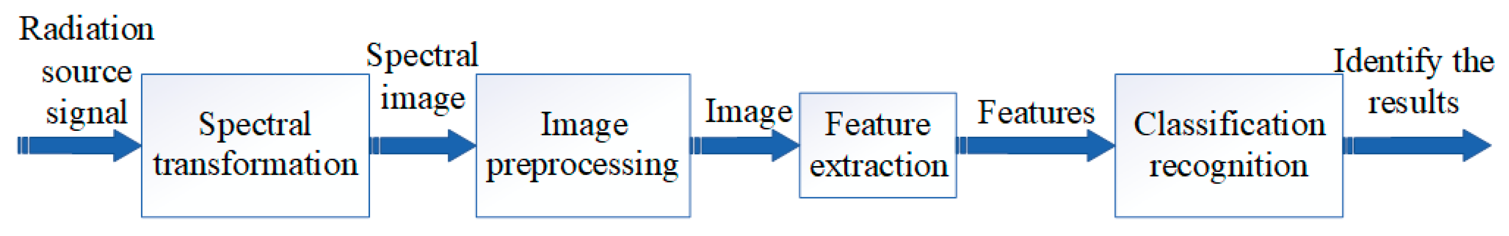
In this paper, a deep-learning method is designed to distinguish the types of radar emitter signals only according to the spectrum images of radar signals. The manually designed neural network is used to automatically extract the features of radar emitter spectrum signals, and then the accurate classification of radar emitter signals is realized according to the obtained features.

(2)

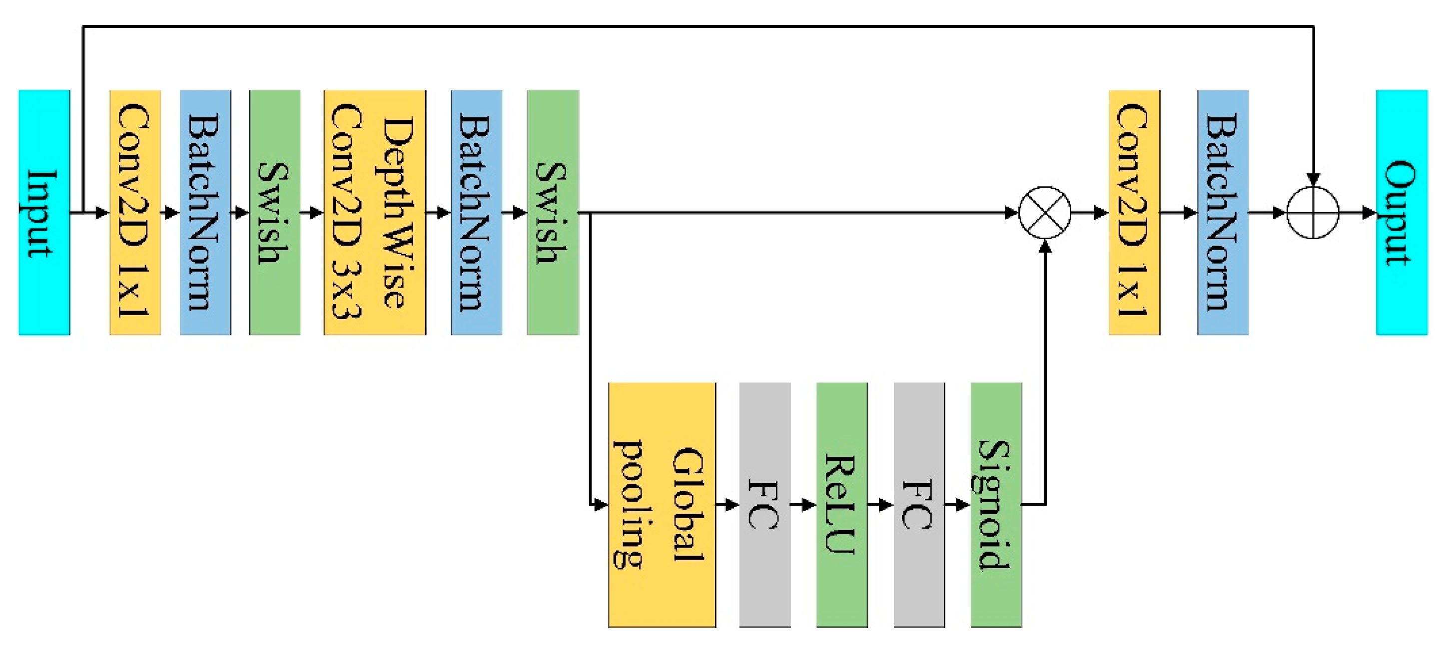
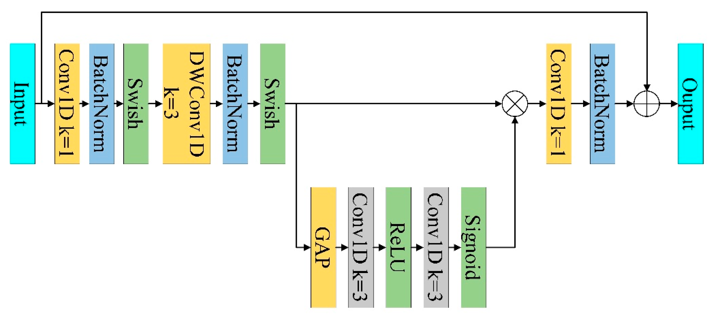
In this paper, considering the characteristics of radar spectrum image, if only two-dimensional convolution is used to extract spectral image features, the local feature similarity is large, and the discrimination degree is not high. Therefore, we use a one-dimensional convolution structure to replace the two-dimensional convolution structure in EfficientNetv2-s. Thus, feature details with a certain degree of discrimination can be extracted, and the number of model parameters and computational complexity can be reduced to a certain extent.

(3)

In this paper, the structure of the attention mechanism in EfficientNetv2-s is modified, the idea of reducing the dimension first and increasing the dimension is abandoned, and the global pooling features are directly implemented through one-dimensional convolution to achieve cross-dimensional information interaction, so as to obtain more targeted attention weights.

2. Related Work

This chapter details the basic theoretical knowledge required by the method proposed in this paper, including the basic knowledge of calculation process of one-dimensional convolution and the basic knowledge of EfficientNetv2.

2.1. 1D Convolution

Convolution is an important part of convolution neural networks. The essence of convolution is to filter the signal, namely, feature extraction. The operation uses weighted average, multiplication and addition to extract useful information from the signal.

In a convolution neural network, the convolution operation can be divided into one-dimensional convolution, two-dimensional convolution and three-dimensional convolution. Among them, 1D convolution only performs a sliding window operation in one direction, which is mostly suitable for processing text data. 2D convolution is a sliding window operation in two directions, which is mostly suitable for processing image data. 3D convolution is a sliding window operation on the cube in three directions, which is mostly suitable for 3D image processing. 1D convolution generally only convolutes the width of the input data but not the height. The specific process is shown in Figure 2.

2.2. EfficientNetv2 Introduction

EfficientNet [22] is a classification network proposed by Mingxing Tan and Quoc V.Le in 2019. The authors searched the EfficientNetB0 structure through neural architecture search (NAS) technology and then used a composite scaling method to uniformly scale the network width, depth and resolution with a composite coefficient, so as to obtain the network structure of EfficientNetB1 to B7. However, there are still great problems in EfficientNet. For example, when the size of the training image is large, the training speed is very slow, and the speed of using depth wise revolutions in the shallow layer of the network will be very slow.

EfficientNetv2 [23] is a smaller and faster network model proposed by Quoc V.Le and others in 2021 to solve the problems of EfficientNet. It also has a faster training speed. EfficientNetv2 is mainly constructed by stacking an inverted linear bottleneck layer with depth-wise separable convolutions (MBConv, as shown in Figure 3) and an inverted fusion residual layer (Fused-MBConv, as shown in Figure 4). The MBConv structure first performs a dimensionality boosting convolution and then uses the depth-wise separable convolution to greatly reduce the number of parameters. Finally, the Squeeze-and-Excitation (SE) module is used to obtain the attention weights, so that the network pays more attention to the useful information in the feature map.

The Fused-MBConv integrates the first two convolution operations of the MBConv structure into a convolution operation with a convolution kernel size of 3, which alleviates the problem of the slow speed of deep convolution. The rest of the operation is similar to the MBConv structure. Unlike EfficientNetv1, EfficientNetv2 searches the model architecture from the search space containing MBConv structure and Fused-MBConv structure and presents an improved progressive learning method. This method can adaptively adjust the regularization operation according to the size of the training image.

3. Efficientnetv2-S Based on One-Dimensional Convolution

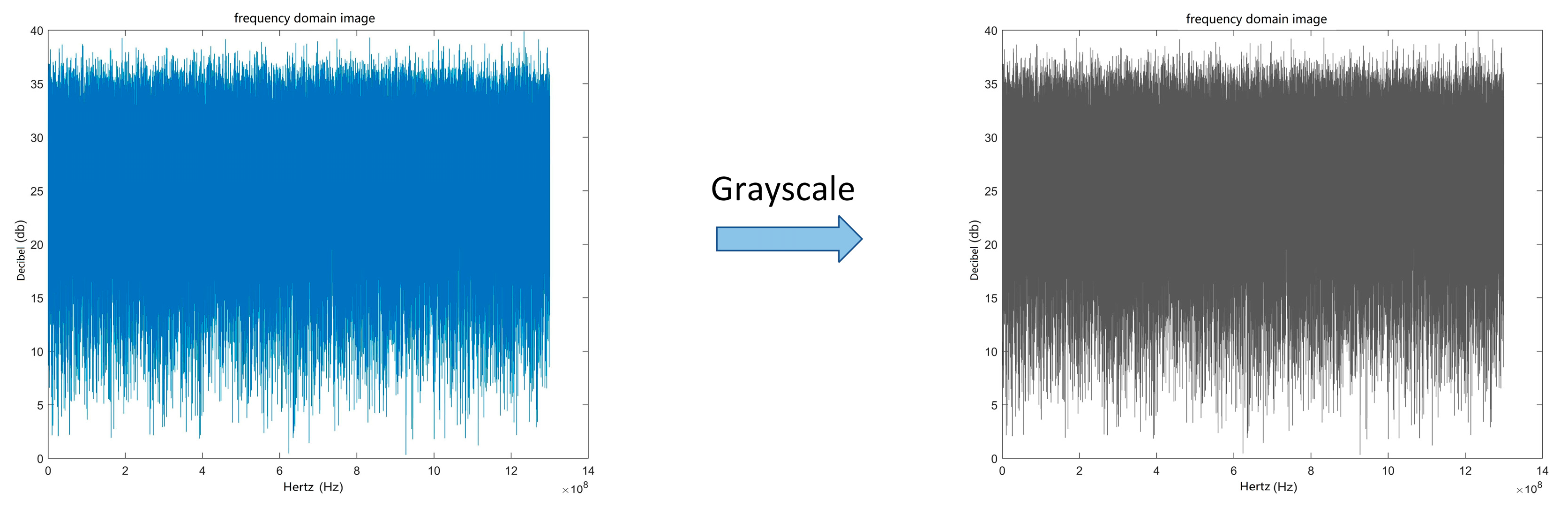
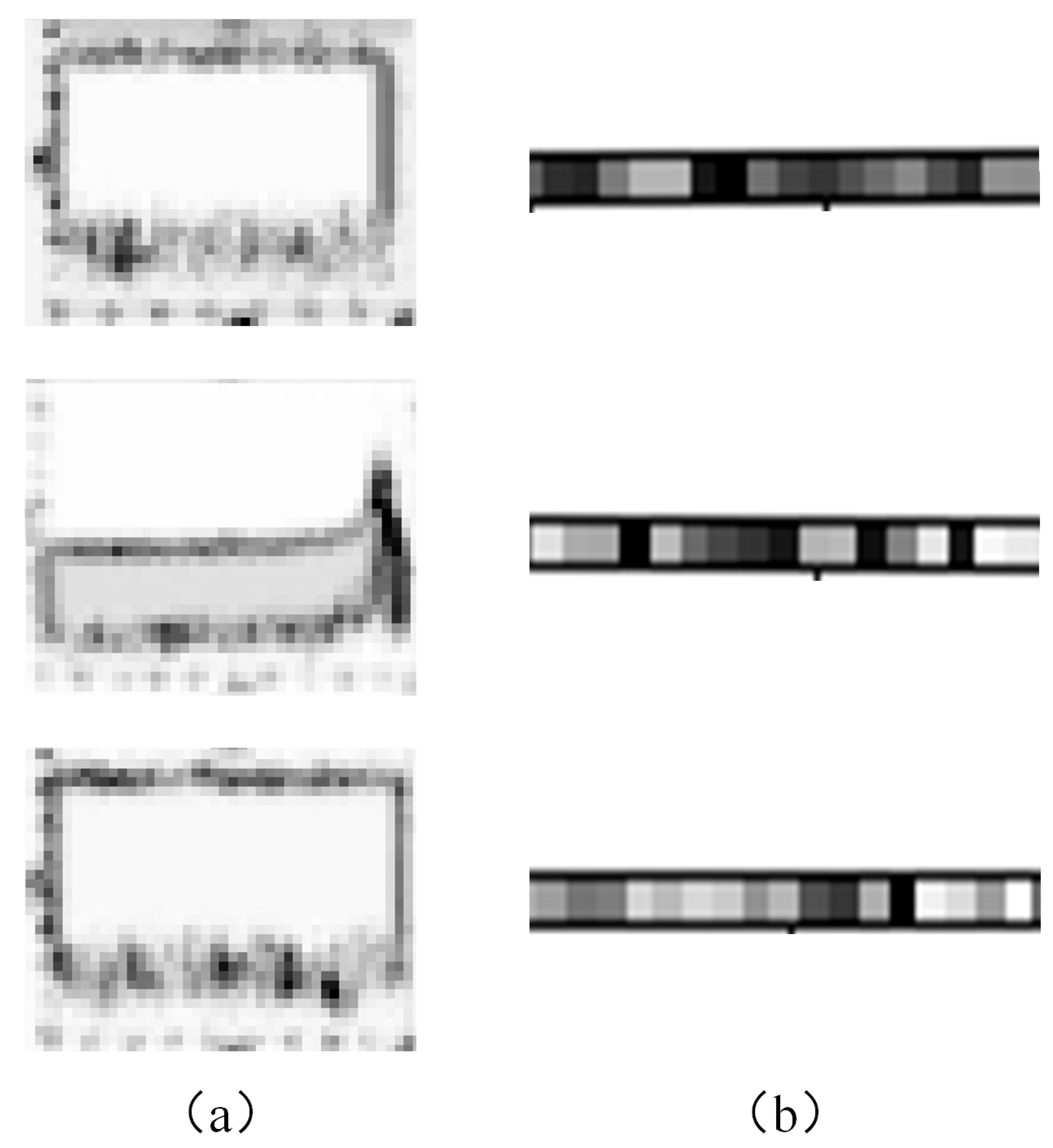
3.1. Data Preprocessing

The image processing in deep learning can be regarded as the processing of multidimensional matrix data. In this paper, considering that the training of radar frequency domain image-classification model is not related to the image color degree of training data, the color image with three channels is read as a single channel gray image, as shown in Figure 5. Since the image processing based on deep learning is equivalent to the processing of multidimensional matrix data, the use of one-dimensional convolution is considered to convolute the image in one direction, in which the input dimension in the one-dimensional convolution for the image is the height of the image.

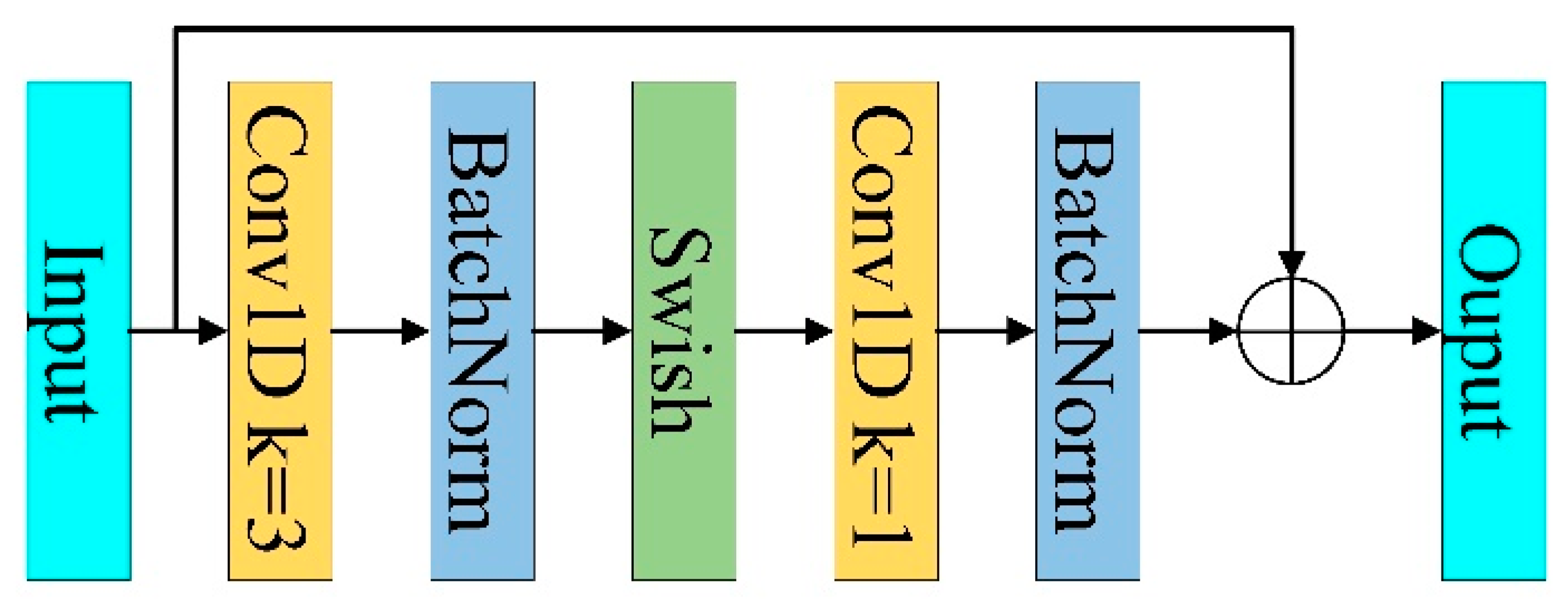
3.2. MBConv and Fused-MBConv Based on One-Dimensional Convolution

In this paper, an EfficientNetv2-s based on one-dimensional convolution is proposed for radar frequency domain image classification. The two-dimensional convolution module in EfficientNetv2-s is replaced by a one-dimensional convolution module. The MBConv structure is changed by using the one-dimensional convolution module. First, the dimension is adjusted through the one-dimensional convolution with the convolution kernel size of 1, then the feature is extracted through a one-dimensional convolution layer with the convolution kernel size of 3, and then the output is used as the input of the attention mechanism.

The attention weight obtained by the attention mechanism is multiplied with the trunk output, and then a convolution operation with a convolution kernel size of 1 is performed to integrate the attention information. Finally, the residual connection is made with the input of MBConv module to obtain the final output as shown in Figure 6. The Fused-MBConv structure is improved by using a one-dimensional convolution module. The idea of improvement is similar to that of modifying MBConv, while the attention module is deleted. The overall structure is shown in Figure 7.

3.3. Improved SE Attention Module

In our proposed method, we modify the SE [24] attention module. Since the dimension reduction operation of SE attention will lead to the loss of some important feature dimensions, we abandon the idea of its own dimension reduction before dimension increase and directly use one-dimensional convolution operation to operate on the global pooling features without dimension reduction, so as to obtain its cross-dimensional related information. Finally, the attention weights are obtained through the Sigmoid layer, so that the modified attention module can obtain more accurate attention weights. The attention module structure used in this paper is shown in Figure 8. First, the features are globally pooled to obtain global information, and then the cross-dimensional related information is obtained by using two layers of one-dimensional convolution operations. Finally, the attention weights are obtained by using the Sigmoid function.

3.4. Our Function

The overall structure of the EfficientNetv2-s method based on one-dimensional convolution proposed in this paper is the repeated stacking of MBConv modules based on one-dimensional convolution and Fused-MBConv modules based on one-dimensional convolution to a certain extent. The overall structure of this model is as shown in

Table 1. EfficientNetv2-s structure based on one-dimensional convolution.

Stage	Operator	Stride
0	Conv1D, k = 3	2
1	Fused-MBConv1D1, k = 3	1
2	Fused-MBConv1D4, k = 3	2
3	Fused-MBConv1D4, k = 3	2
4	MBConv1D4, k = 3, SE	2
5	MBConv1D6, k = 3, SE	1
6	MBConv1D6, k = 3, SE	2
7	Conv1D, k = 1 and Pooling and FC	-

, where the number after the module represents the number of consecutive stacking times of the module, k represents the size of the convolution kernel of the main convolution in the module, and SE represents the improved attention module.

The feature map extracted by EfficientNetv2-s and the feature map extracted by our method are shown in Figure 9. We can see that the features extracted by EfficientNetv2-s in (a) are standard image features, but there are too many similar parts in the feature map, resulting in difficulties in the subsequent extraction of discriminative features. In (b), parts of the features extracted by our method are shown. The two-dimensional image features are extracted in a dimension direction, and the extracted features are more discriminative.

4. Experiment

In this chapter, we introduce the selected data sets, experimental methods, experimental settings and experimental results in detail. We compare the results with other classification models.

4.1. Data Set

The data set used in this experiment is the spectrum images with different amplitude sizes randomly generated according to the radar signal parameter table. The data set contained 16 categories, each category had 50 pictures, and the picture size was 7500 × 5236. In each category, 40 images were randomly selected as the training set and verification set data, 90% of which were the training set and 10% were the verification set. The remaining images in each category were used as the test set data for the final verification and evaluation of the model effect. During the experiment, the spectrum image was divided into small blocks with a width of 224 to increase the number of data sets and increase the diversity of data.

4.2. Experimental Setup

When building the data loader, the image data was directly read as a gray-scale image, and the image size was scaled proportionally. As the structure of the model changed, the pre-training model was not used. During the training, the batch size of each input was 8, the SGD was selected as the optimizer, the initial learning rate was set to 0.01, and the momentum was set to 0.9. A total of 100 iterations of training were performed. The model with stable convergence of loss function was selected as the final classification model. The same experimental setup was used to train other deep-learning models widely used in classification tasks using the same data preprocessing.

The models used for comparison are all based on two-dimensional convolution. Top1 accuracy, top5 accuracy and FLOPs were selected as evaluation indexes in this experiment. Top1 accuracy refers to the accuracy rate of the category ranked first in classification prediction probability and the actual result. Top5 accuracy refers to the accuracy of including the actual results in the top five categories with the classification prediction probability. FLOPs refers to floating-point numbers that can be understood as computational quantities, used here to measure the model complexity.

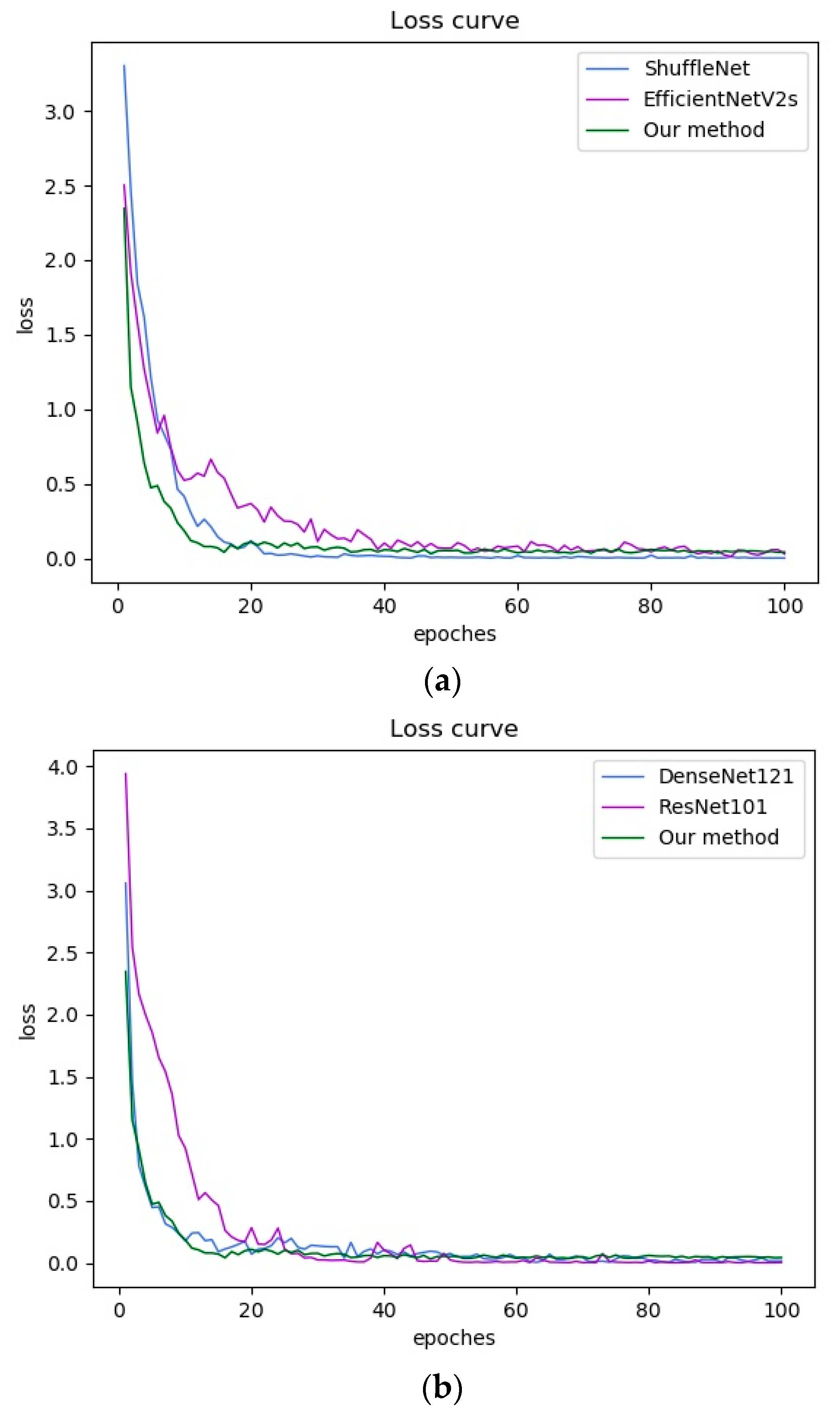
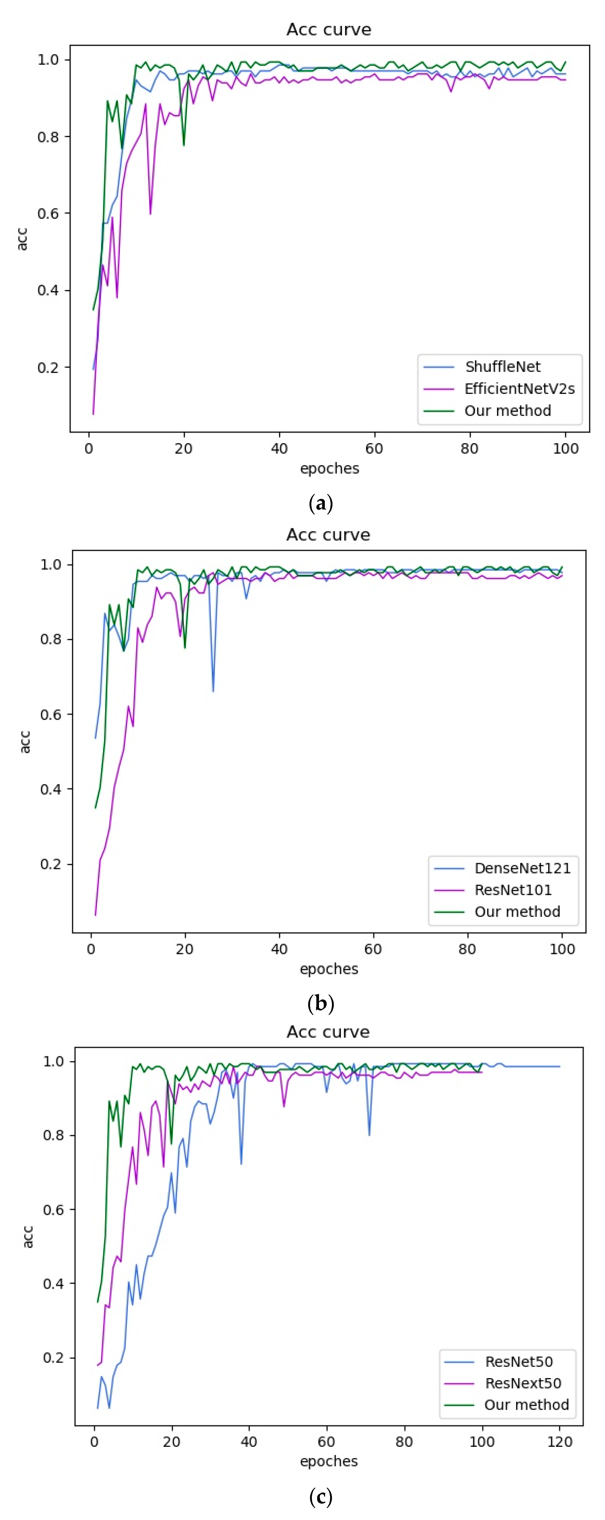
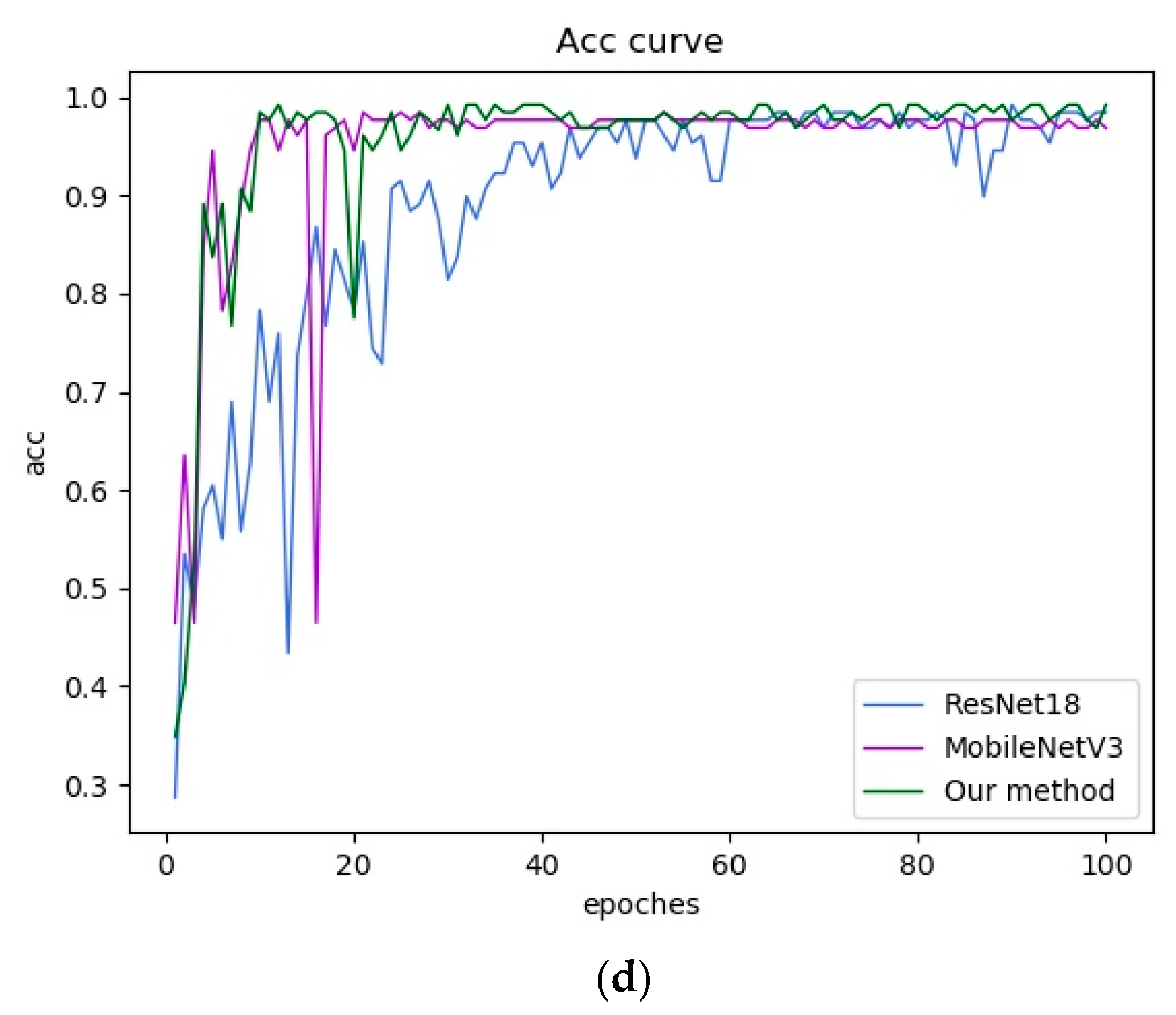
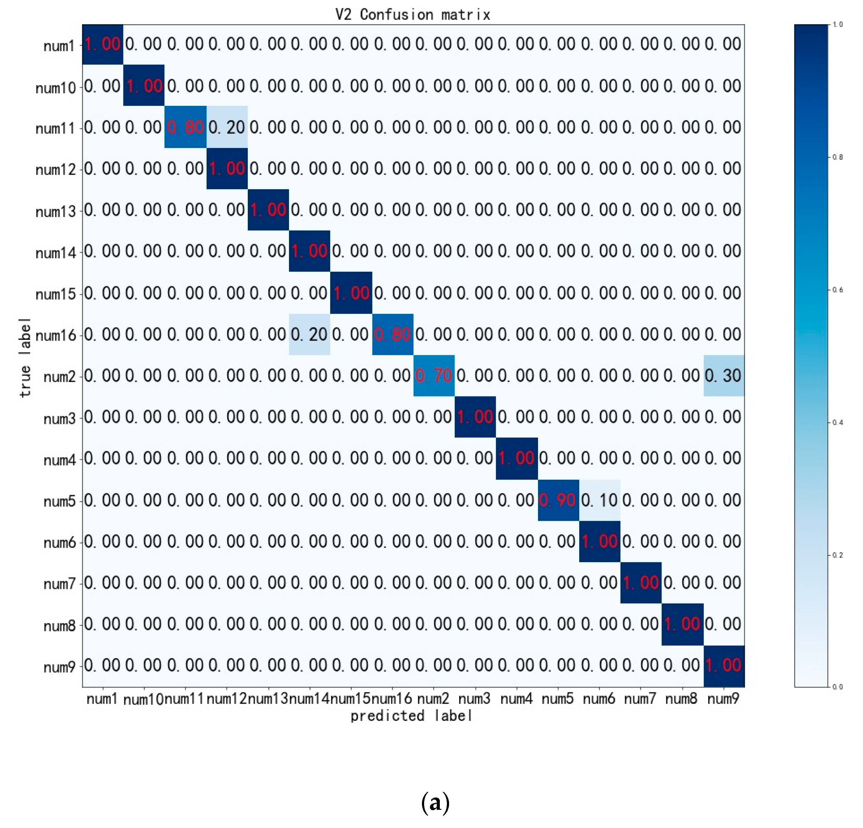
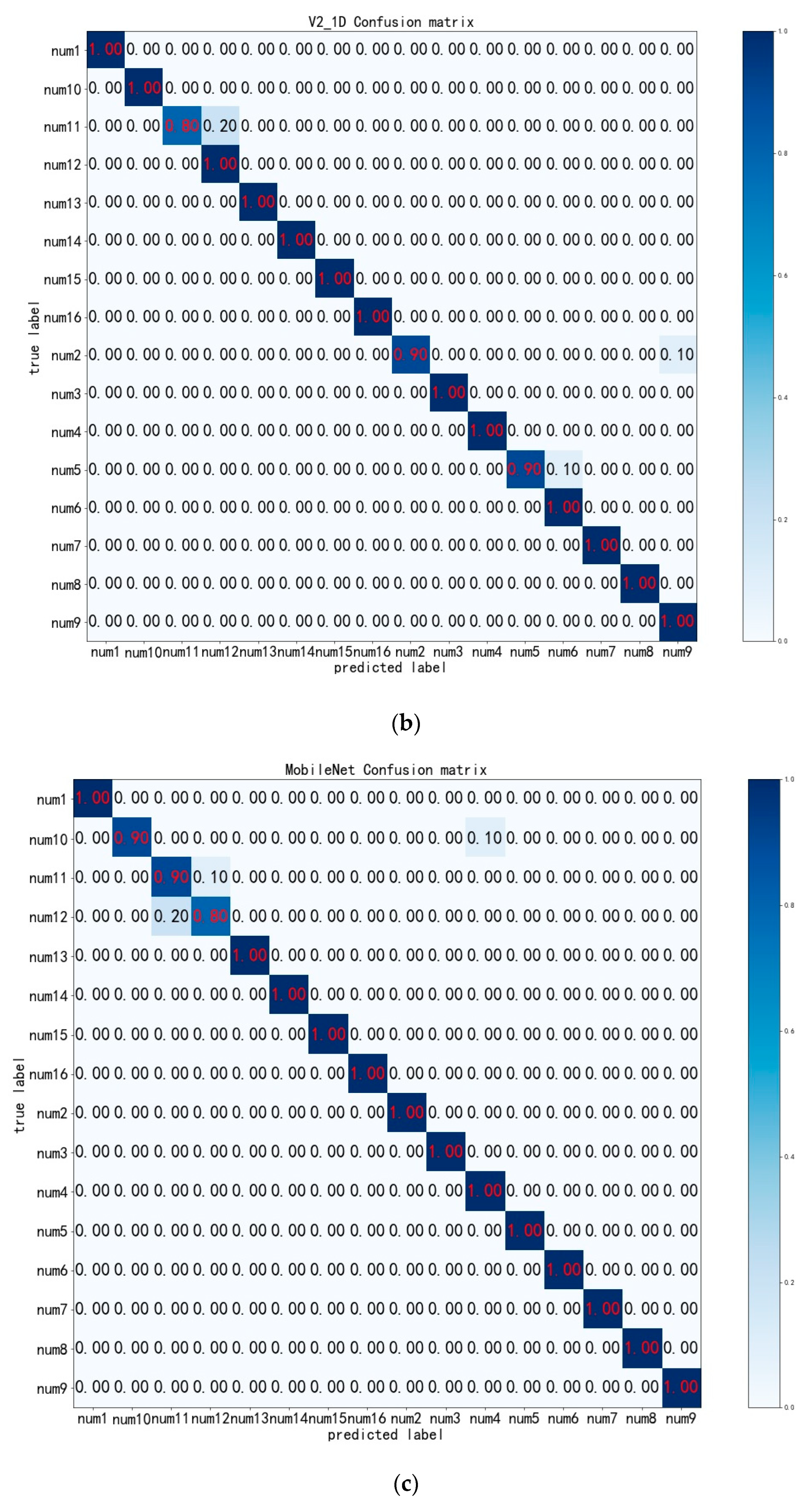
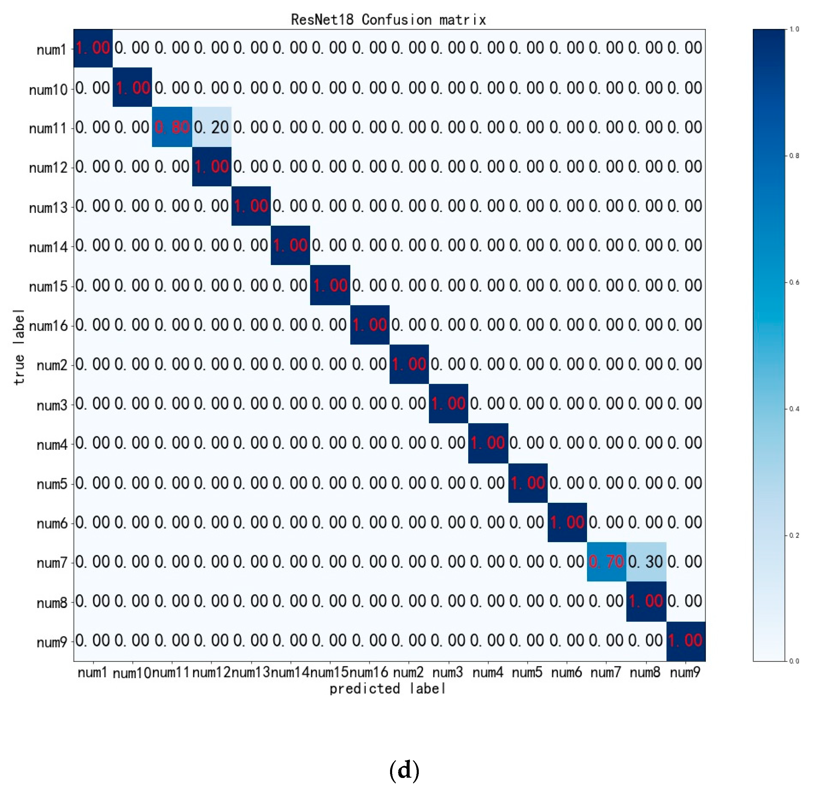
4.3. Experimental Results and Analysis

The loss function of each model during training is shown in Figure 10, where (a) is the comparison of our method with the loss function of EfficientNetv2-s and ShuffleNet, (b) is the comparison of our method with the loss function of ResNet101 and DenseNet121, (c) is the comparison of the loss function of our method with ResNet50 and ResNeXt50 and (d) is the comparison of the loss function of our method with ResNet18 and MobileNetV3. All the loss functions were cross-entropy loss functions.

The classification accuracy of each model on the validation set is shown in Figure 11, where (a) is the top1 accuracy comparison of our method with EfficientNetV2-S and ShuffleNet on the validation set, (b) is the top1 accuracy comparison of our method with ResNet101 and DenseNet121 on the validation set, (c) is the top1 accuracy comparison of our method with ResNet50 and ResNeXt50 on the validation set, and (d) is the top1 accuracy comparison of our method with ResNet18 and MobileNetV3 on the validation set.

Based on the above loss function images and the accuracy images of the validation set, compared with other methods, the loss values of our method can converge rapidly during training, and the convergence speed is better than most experimental models. Figure 11 shows the accuracy changes of each model on the validation set during the training process in order to better view the training situation of the model. In Figure 11b, the validation set accuracy of our proposed method and DenseNet121 both reach a high level.

Although the verification accuracy of our proposed method fluctuates somewhat, it is slightly higher than that of the DenseNet121. In Figure 11d, the accuracy of our proposed method on the validation set is higher than those of ResNet18 and MobileNetV3 on the validation set.

Table 2. Top1 accuracy, top5 accuracy and FLOPs of each method on the test set.

Method	Input Size	FLOPs	Top1 Accuracy	Top5 Accuracy
MobileNetV3	224 * 224	0.059 G	97.96 ± 0.05%	100%
ResNet-18	224 * 224	1.740 G	96.89 ± 0.15%	100%
ResNet-50	224 * 224	3.798 G	96.87 ± 0.25%	100%
ResNet-101	224 * 224	7.521 G	96.87 ± 0.25%	99.3 ± 0.2%
ResNeXt-50	224 * 224	6.658 G	95.62 ± 0.15%	100%
DenseNet-121	224 * 224	2.787 G	96.87 ± 0.05%	100%
ShuffleNet	224 * 224	0.142 G	95.00 ± 0.15%	100%
EfficientNetv2-s	224 * 224	5.342 G	95.00 ± 0.15%	100%
Our method	224 * 224	0.212 G	98.12 ± 0.25%	100%

shows the final test results of each method on the test set. Although MobileNetV3 has very low FLOPs, its top1 accuracy is still slightly lower than the final results of our proposed method on the test set.

The evaluation results of each method on the radar frequency domain image test set are shown in Table 2. The top1 accuracy and top5 accuracy data are the average values of five experiments conducted by each model on the experimental data set. According to the data in the table, it is obvious that the classification and detection results of our method on the radar frequency domain image test set are better than other methods. In terms of classification accuracy, our method improved the top1 accuracy by about 3% compared with EfficientNetv2-s and improved the top1 accuracy by about 1.5% compared with ResNet18, but the accuracy improvement is low compared with MobileNetv3. These show the effectiveness of our method in the classification and recognition of emitter signals. At the same time, with the improvement of accuracy, the FLOPs of the proposed method model were reduced from 5.432 G of EfficientNetv2-s to 0.212 G, which greatly reduces the complexity of the model.

The confusion matrix of some models’ test results on the test set is shown in Figure 12, where (a) is the confusion matrix of our proposed methods, (b) is the confusion matrix of the EfficientNetv2-s, (c) is the confusion matrix of MobileNetv3, and (d) is the confusion matrix of ResNet18. In the confusion matrix, darker colors have higher values. It can be intuitively seen from the confusion matrix that our method can achieve accurate classification of various types of radar signals.

The parameter quantities of each model are shown in

Table 3. Comparison of the parameters of each model.

Method	Params
MobileNetV3	1.85 M
ResNet-18	11.17 M
ResNet-50	37.59 M
ResNet-101	23.53 M
ResNeXt-50	42.53 M
DenseNet-121	7.97 M
ShuffleNet	1.26 M
EfficientNetv2-s	20.21 M
Our method	19.47 M

. Through the comparison of parameter quantities, the method in this paper had a partial reduction in parameter quantities compared with EfficientNetv2-s with a reduction of about 0.8 M.

According to the analysis of the above experimental results, the method of radar emitter signal classification and recognition based on deep learning proposed in this paper had a good effect in the test set, and the recognition accuracy was as high as 98.12%. The complexity of the proposed model method was analyzed. The complexity analysis was mainly discussed from the aspects of FLOPs and parameter quantity. In terms of calculation quantity, the FLOPs of the proposed method were far less than those most of other experimental models from Table 2. In terms of the parameter quantity, the proposed method was improved compared with EfficientNetv2-s. While the parameter quantity was only reduced by 0.8 M, this is still less than EfficientNetv2-s and ResNeXt-50. Overall, the complexity of the proposed method was less than most other models.

5. Conclusions

This paper presented a method of emitter classification and recognition based on deep learning, which was an EfficientNetv2-s convolution structure model based on one-dimensional convolution. This method can obtain the input image suitable for the neural network by scale compression and gray processing of frequency domain image in the data set. Then, the features are extracted by the stacked one-dimensional convolution and attention modules to achieve accurate classification and recognition of radar radiation sources. For the research data set, a variety of other models were selected to set up comparative experiments, which proved the good performance of the proposed method in the recognition and classification of radiation sources.

Although this method had good classification performance on the experimental data set, it still has some shortcomings and can be improved. The first deficiency is the data set. Since the data set was made by us, the generalization and robustness of this method in other research fields need to be studied. The second deficiency is that the proposed method model has the possibility of further simplification and does not achieve lightweight treatment of the model. The third disadvantage is that the proposed method is only applicable to the case that the training data and test data come from the same working conditions. If the working conditions change, the distribution of sample data will change, which will lead to a decline in test accuracy. Further research will focus on the generalization and improvement of the proposed method and lightweight treatment of the model.

References

1. Tang, J.-R.; Zhu, Y.-Q.; Xu, Q. Study of Radar Emitter Recognition by Using Neural Networks. J. Air Force Radar Acad. 2007, 21, 25–27. [Google Scholar]
2. Wei, Q.; Ping, L.; Xu, F. An algorithm of signal sorting and recognition of phased array radars. In Proceedings of the IEEE 10th International Conference on Signal Processing Proceedings, Beijing, China, 24–28 October 2010. [Google Scholar]
3. Hu, K.; Wang, H.-Y. Decision Tree Radar Emitter Recognition Based on Rough Set. Comput. Simul. 2011, 28, 4. [Google Scholar]
4. Guan, X.; Guo, Q.; Zhang, Z.-C. Radar Emitter Signal Recognition Based on Kernel Function SVM. J. Proj. Rocket. Missiles Guid. 2011, 31, 4. [Google Scholar]
5. Kvasnov, A. Methodology of classification and recognition the radar emission sources based on Bayesian programming. IET Radar Sonar Navig. 2020, 14, 1175–1182. [Google Scholar] [CrossRef]
6. Xiao, W.; Wu, H.; Yang, C. Support vector machine radar emitter identification algorithm based on AP clustering. In Proceedings of the 2013 International Conference on Quality, Reliability, Risk, Maintenance, and Safety Engineering (QR2MSE), Chengdu, China, 15–18 July 2013. [Google Scholar]
7. Zhu, X.-L.; Cai, Q.; Zhou, M.-L. Radar Radiation Source Identification Based on BP Neural Net and Bayes Reasoning. Shipboard Electron. Countermeas. 2012, 35, 4. [Google Scholar]
8. Matuszewski, J.; Sikorska-Lukasiewicz, K. Neural network application for emitter identification. In Proceedings of the International Radar Symposium, Prague, Czech Republic, 28–30 June 2017; pp. 1–8. [Google Scholar]
9. Liu, K.; Wang, J.-G. An Intelligent Recognition Method Based on Neural Network for Unknown Radar Emitter. Electron. Inf. Warf. Technol. 2013, 28, 5. [Google Scholar]
10. Zhu, W.; Meng, L.; Zeng, C. Research on Online Learning of Radar emitter identification Based on Hull Vector. In Proceedings of the IEEE Second International Conference on Data Science in Cyberspace, Shenzhen, China, 26–29 June 2017. [Google Scholar]
11. Tang, X.-J.; Chen, W.-G.; Xi, L.-F. The Radar Emitter Identification Algorithm Based on AdaBoost and Decision Tree. Electron. Inf. Warf. Technol. 2018, 33, 6. [Google Scholar]
12. Jin, Q.; Wang, H.; Yang, K. Radar emitter identification based on EPSD-DFN. In Proceedings of the 2018 IEEE 3rd Advanced Information Technology, Electronic and Automation Control Conference (IAEAC), Chongqing, China, 12–14 October 2018. [Google Scholar]
13. Guo, Q.; Nan, P.; Wan, J. Signal classification method based on data mining for multi-mode radar. J. Syst. Eng. Electron. 2016, 27, 1010–1017. [Google Scholar] [CrossRef]
14. Tang, J.; Zhu, J.; Zhao, Y. Automatic recognition of radar signals based on time-frequency image character. In Proceedings of the IET International Radar Conference 2013, Xi’an, China, 14–16 April 2013. [Google Scholar]
15. Wu, J.-C.; Qu, Z.-Y.; Chen, X. Radar emitter signal recognition method based on time-frequency energy distribution. J. Air Force Early Warn. Acad. 2020, 34, 4. [Google Scholar]
16. Tavakoli, E.T.; Falahati, A. Radar Signal Recognition by CWD Picture Features. Int. J. Commun. Netw. Syst. Sci. 2012, 5, 238–242. [Google Scholar] [CrossRef]
17. Liang, H.; Han, J. Sorting Radar Signal Based on Wavelet Characteristics of Wigner-Ville Distribution. J. Electron. 2013, 30, 454–462. [Google Scholar] [CrossRef]
18. Ye, W.-Q.; Yu, Z.-F. Signal Recognition Method Based on Joint Time-Frequency Radiant Source. Electron. Inf. Warf. Technol. 2018, 33, 5. [Google Scholar]
19. Lunden, J.; Koivunen, V. Automatic Radar Waveform Recognition. IEEE J. Sel. Top. Signal Process. 2007, 1, 124–136. [Google Scholar] [CrossRef]
20. Xin, W.; Xu, W.; Wei, H. Radar Emitter Recognition Algorithm Based on Two-dimensional Feature Similarity Coefficient. Shipboard Electron. Countermeas. 2020, 43, 7. [Google Scholar]
21. Hinton, G.E.; Osindero, S.; The, Y.W. A Fast Learning Algorithm for Deep Belief Nets. Neural Comput. 2006, 18, 1527–1554. [Google Scholar] [CrossRef] [PubMed]
22. Tan, M.; Le, Q.-V. EfficientNet: Rethinking Model Scaling for Convolutional Neural Networks. In Proceedings of the 36th International Conference on Machine Learning (ICML 2019), Long Beach, CA, USA, 10–15 June 2019. [Google Scholar]
23. Tan, M.; Le, Q.-V. EfficientNetV2: Smaller Models and Faster Training. In Proceedings of the 38th International Conference on Machine Learning, Virtual, 18–24 July 2021. [Google Scholar]
24. Jie, H.; Li, S.; Gang, S. Squeeze-and-Excitation Networks. IEEE Trans. Pattern Anal. Mach. Intell. 2017, 42, 2011–2023. [Google Scholar]
Figure 1. Flow of radiation source signal classification.
Electronics 12 02110 g001
Figure 2. One-dimensional convolution flow, where * stands for convolution operation.
Electronics 12 02110 g002
Figure 3. MBConv structure diagram. The dark blue module represents standardization, the yellow module represents convolution and pooling operations, the green module represents the activation function, and the grey module represents the fully connected layer.
Electronics 12 02110 g003
Figure 4. Fused-MBConv structure diagram. The dark blue module represents standardization, the yellow module represents convolution and pooling operations, the green module represents the activation function, and the grey module represents the fully connected layer.
Electronics 12 02110 g004
Figure 5. Conversion from a color image to a gray image.
Electronics 12 02110 g005
Figure 6. MBConv structure based on conv1d. Where yellow module represents the convolution operation, dark blue module represents the normalization operation, green module represents the activation function, and gray module represents the convolution operation used to replace the fully connected layer.
Electronics 12 02110 g006
Figure 7. Fused-MBConv structure based on conv1d. The yellow module represents the convolution operation, the dark blue module represents the normalization operation, and the green module represents the activation function operation.
Electronics 12 02110 g007
Figure 8. Modified structure of the SE attention.
Electronics 12 02110 g008
Figure 9. Feature map extracted by two methods. Where (a) is the visualization of features extracted using 2D convolution operators, and (b) is the visualization of features extracted using 1D convolution operators.
Electronics 12 02110 g009
Figure 10. Comparison of loss functions of various models. Where (a) is the loss decline curve comparison of ShuffleNet, EfficientNetV2s and our method, (b) is the loss decline curve comparison of DenseNet121, ResNet101 and our method, (c) is the loss decline curve comparison of ResNet50, ResNext50 and our method, (d) is the loss decline curve comparison of ResNet18, MobileNetV3 and our method.
Electronics 12 02110 g010aElectronics 12 02110 g010b
Figure 11. Comparison of the accuracy of each model validation set. Where (a) is the accuracy curve comparison of ShuffleNet, EfficientNetV2s and our method, (b) is the accuracy curve comparison of DenseNet121, ResNet101 and our method, (c) is the accuracy curve comparison of ResNet50, ResNext50 and our method, (d) is the accuracy curve comparison of ResNet18, MobileNetV3 and our method.
Electronics 12 02110 g011aElectronics 12 02110 g011b
Figure 12. Confusion matrix of the partial model. Where (a) is the confusion matrix of our proposed, (b) is the confusion matrix of EfficientNetV2s, (c) is the confusion matrix of MobileNetV3, (d) is the confusion matrix of ResNet18. Where red is the accuracy of the predicted classification.
Electronics 12 02110 g012aElectronics 12 02110 g012bElectronics 12 02110 g012c