InSEption: A Robust Mechanism for Predicting FoG Episodes in PD Patients

Abstract

The integration of IoT and deep learning provides the opportunity for continuous monitoring and evaluation of patients’ health status, leading to more personalized treatment and improved quality of life. This study explores the potential of deep learning to predict episodes of freezing of gait (FoG) in Parkinson’s disease (PD) patients. Initially, a literature review was conducted to determine the state of the art; then, two inception-based models, namely LN-Inception and InSEption, were introduced and tested using the Daphnet dataset and an additional novel medium-sized dataset collected from an IMU (inertial measuring unit) sensor. The results show that both models performed very well, outperforming or achieving performance comparable to the state-of-the-art. In particular, the InSEption network showed exceptional performance, achieving a 6% increase in macro F1 score compared to the inception-only-based counterpart on the Daphnet dataset. In a newly introduced IMU dataset, InSEption scored 97.2% and 98.6% in terms of F1 and AUC, respectively. This can be attributed to the added squeeze and excitation blocks and the domain-specific oversampling methods used for training. The benefits of using the Inception mechanism for signal data and its potential for integration into wearable IoT are validated.

1. Introduction

Neurodegenerative diseases such as Alzheimer’s disease, Parkinson’s disease, and multiple sclerosis are chronic and progressive disorders that are characterized by the gradual and ongoing death of neurons, leading to a variety of motor and cognitive symptoms that can significantly impact a patient’s quality of life. Parkinson’s disease, in particular, has both motor and non-motor symptoms, with freezing of gait (FoG) being a significant and persistent symptom that can result in decreased mobility and an increased risk of falls.

Diagnosis of Parkinson’s disease typically relies on score-based tests that evaluate the progression of symptoms, including motor and cognitive functions. These tests can include the Unified Parkinson’s Disease Rating Scale (UPDRS) and the Movement Disorder Society-Unified Parkinson’s Disease Rating Scale (MDS-UPDRS). FoG is a challenging symptom to diagnose and monitor due to its unpredictable nature. Therefore, continuous monitoring is necessaryto identify the optimal course of treatment that can minimize the effects of the condition on the patient’s daily activities and overall mobility. Recent advances in smart phones have enabled the use of sensors such as accelerometers to detect and monitor FoG and provide real-time feedback on gait patterns. The ability to provide continuous monitoring and collect data can assist clinicians in comprehending the frequency and intensity of FoG episodes, thereby enabling them to effectively customize treatment plans.

Moreover, automatically identifying FoG episodes can significantly reduce the workload of medical personnel, who previously had to manually review video footage of each patient. Additionally, it can provide valuable analytics and early warning systems to alert caregivers when an episode occurs.

To predict FoG episodes, various methods have been proposed, such as fixed thresholds and advanced deep neural network models. Machine learning and deep learning techniques have shown better performance compared to other methods, despite the complexity of sensor readings and the unpredictable nature of FoG episodes [1,2,3]. Specifically, several successful attempts have been made utilizing data derived from sensors and applying a selection of machine and deep learning methods in order to identify FoG episodes [4,5,6,7,8,9,10]. Common architectures such as LSTMs, CNNs, and combinations of both have been used, and an inception based model was developed [11]. Finally, most studies have not validated their methods across multiple datasets, providing no evidence that the suggested model’s performance would be consistent on other datasets.

This study presents a modified inception base framework with easily adjustable hyperparameters, providing a more generic approach to detect FoG episodes. Specifically, the immediate contributions of this work are as follows:

• The introduction of two novel inception-based models, namely InSEption and LN-Inception;
• A comparison of the iSPLInception model [11] and the proposed methods on the Daphnet dataset;
• A comparison of the proposed models on a previously unused dataset by Ribeiro De Souza et al. [12].

This paper is organized into several sections. In Section 2, we present existing methodologies and the current state of the art in FoG detection. Section 3 describes the datasets used in the study, as well as the proposed network architectures. Next, in Section 4, we present the results of the conducted experiments and provide details about the proposed methodologies. Finally, in Section 5, we provide concluding remarks on the study and highlight observations and recommendations for future research.

2. Related Work

The Daphnet dataset is a widely used benchmark dataset for the detection of FoG in individuals with Parkinson’s disease. It was developed as part of a study by Bachlin et al. [13] and consists of data from three sensors measuring the gait of ten patients with Parkinson’s disease. Their proposed system for online detection of FoG was based on frequency components of movements and achieved sensitivity and specificity of 73.1% and 81.6%, respectively. Subsequent studies by the same authors showed potential to improve these metrics to 85.9% and 90.9%, respectively.Furthermore, the system provides auditory guidance and a distinct sound when an episode is detected.

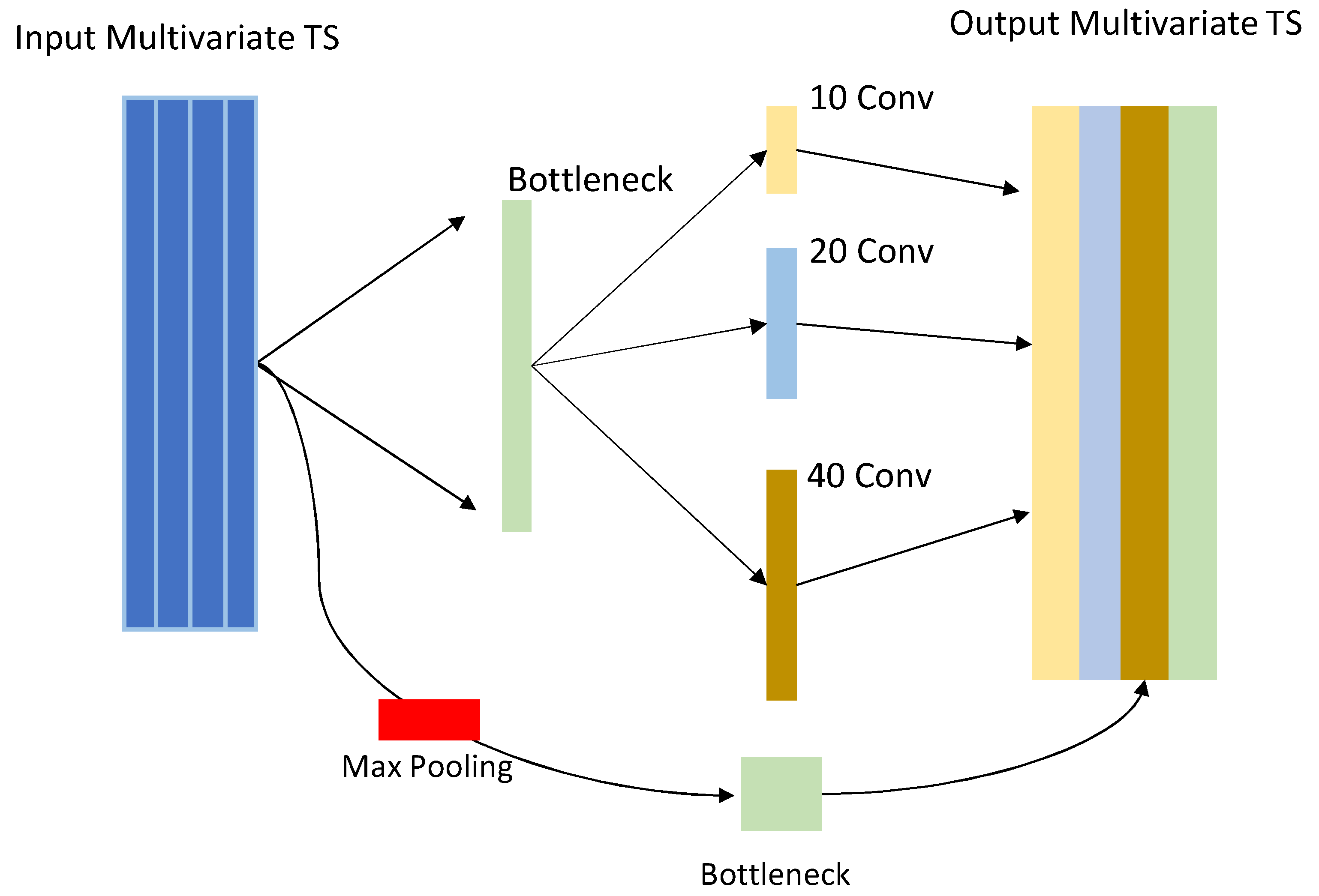
In [11], the authors proposed a new deep learning architecture for FoG detection based on the Inception Res-net model introduced by Google, which utilizes 1D convolution and MaxPooling in parallel. The output is then fed to different convolution layers with varying dimensions and a 1x1 convolutional layer. To evaluate the performance of iSPLInception, tests were conducted on various human activity recognition datasets, including the Daphnet dataset, which was split into specific training, validation, and test sets. The iSPLInception model outperformed the other deep learning methodologies, with an F1 score of 94% on the test set.

Moreover, a deep learning model called DeepFoG was developed in [4], for detection of freezing of gait (FoG) episodes in Parkinson’s disease patients using wrist-worn IMU sensors, which allows for the easy deployment of the proposed system. The authors compared their proposed methodology to decision trees and XGBoost and found that the DeepFoG model outperformed the other models, achieving 90% specificity and sensitivity on a 10-KFold validation and 88% and 83%, respectively for LOSO CV.

In [14], the authors aimed to identify FoG episodes using the Daphnet dataset. They employed several machine learning models, along with different preprocessing steps, achieving an improvement in sensitivity compared to the literature. They reported that the best overall model was an ensemble method, but it is unclear whether the impact of the prepossessing methods had any effects on performance.

Similarly, in [5], different convolutional LSTM architectures were developed to identify FoG occurrences. The best model was composed of a combination of 1D convolutional layers, squeeze and excitation blocks, and attention-enhanced LSTM layers. The authors evaluated the performance of their model using two techniques: leave one subject out (LOSO) and 10-fold cross validation. Furthermore, they used data augmentation to balance FoG and non-FoG episodes, although the exact method used was not mentioned. The final results indicated that the proposed deep neural network can outperform the competition in terms of both sensitivity and specificity for the R10Fold and in AUC (0.945) for the LOSO validation.

Tautan et al. [6] developed a similar approach to detect FoG episodes using the Daphnet dataset as in [5]. They utilized a deep convolutional network based on AlexaNet. The network consisted of five 1D convolutional layers; three dense layers; and several dropout, batch normalization, and pooling layers. In this case, 10-KFold cross validation was used, with nine of the samples used for training and one used for testing. Overall, the best results were acquired from a balanced dataset, with the algorithm achieving a mean specificity of 83.77% and a mean sensitivity of 81.78%.

In [15], an autoencoder was developed to denoise and enrich accelerometer and gyroscope data for FoG detection. The autoencoder consisted of 15 layers of 1D convolutional, max-pooling, and upsampling layers. The output of the autoencoder was used as input to several machine learning algorithms, including naive Bayes, SVMs, random forest, and ensemble models for FoG or non-FoG episode classification. The random forest model achieved the best performance, with a sensitivity of 90.94% and specificity of 67.04%, using a 2-s window and replacing extreme values in the signal with the mean of the time series (four-sigma rule).

Hssayeni et al. [8] proposed a more sophisticated model than those presented in previous studies by employing an ensemble of models to predict motor performance, as measured by the UPDRS-III test. The dataset used in their study consisted of measurements taken from two sensors located on the wrist and ankle of 24 patients (PAMAP2). The authors employed three different models in their ensemble, including a dual-channel LSTM trained using transfer learning and two CNN-LSTMs (one using one-dimensional convolution and the other using two-dimensional convolution). In addition to the raw signal and frequency-related features, one of the models also included manually created features. The predictions of the three models were then averaged to produce the final UPDRS-III score. The evaluation metrics used were correlation and mean absolute error, which achieved $\rho$ = 0.79 and 5.95, respectively. These results demonstrated that the ensemble models were highly effective in predicting the UPDRS score.

In [9], a bidirectional LSTM network was used to predict the risk of falls in patients with multiple sclerosis using data from gyroscopic and accelerometer measurements collected from sensors placed on patients’ core and legs. They compared the performance of various machine learning models, and the best results were obtained with the Bi-LSTM model.

In ref. [7], the authors utilized, two- and three-layer LSTMs to detect freezing-of-gait (FoG) episodes in Parkinson’s disease patients using plantar pressure data. The models were validated using one-freeze-held validation, and the two-layered LSTM was found to be superior.

Finally, the authors of ref. [10] used transfer learning to develop LSTM models to predict FoG events in Parkinson’s disease patients using the Daphnet dataset. Their second scheme of transfer learning consistently outperformed the existing recurrent model, with an accuracy score over 90% in all prediction horizons and subjects’ training data percentages.

Most of the related works in this field rely on IMU sensors to identify Parkinson’s disease (PD)-related symptoms. However, other types of sensors are also capable of identifying these symptoms. For instance, Farhani et al. [16] used data from 15 patients wearing an EMG sensor to train a Bi-LSTM. They employed a regularized evolutionary algorithm to set the hyperparameters of the model instead of doing so manually. Their objectives were to classify the tasks each patient was conducting and to detect PD-related tremors. Their results showed that the mean achieved accuracy for both tasks was over 84%, which is well above chance levels. Cole et al. [17] used a similar type of sensor, in addition to accelerometer readings, to identify freezing-of-gait (FoG) episodes. They employed a DNN, which achieved a sensitivity of 83% and a specificity of 97% on a per-second basis.

Research shows that deep learning architectures have achieved significant success in detecting FoG episodes, especially when combined with certain preprocessing methods. Among the state-of-the-art architectures used for FoG detection, convolutional and recurrent neural networks are considered the most effective. Convolutional networks offer the advantage of automatically identifying and extracting features without the need for manual feature engineering. On the other hand, recurrent networks are able to capture long-term dependencies in the data and are therefore often effective predictors. In addition to these architectures, attention mechanisms are also commonly used to further weight the connections within the network. Combining all these methodologies can achieve state-of-the-art results, as demonstrated in a recent study [5].

However, it is worth noting that the Daphnet dataset is commonly used as a benchmark in FoG detection research, despite being relatively small. There is a clear need for larger datasets with more patients to bridge this gap. A new dataset introduced by Ribeiro De Souza et al. [12] containing data from IMU sensors from 35 patients aims to address this issue.

Moreover, it is observed that most studies employ a single dataset to evaluate their proposed model. It would be beneficial for future research to evaluate models on multiple datasets to ensure their effectiveness across different patient populations and settings.

The selection of IMU datasets was primarily influenced by their widespread availability in wearable devices, which allows for continuous monitoring of patients without requiring special equipment or environments. Medical advisors of the ALAMEDA project also recommended the use of a particular sensor due to the clinical focus of the project to investigate digital biomarkers using these type of sensors in home environments. Moreover, IMUs have been extensively used in previous studies to monitor Parkinson’s disease symptoms compared to other types of sensors [18]. Finally, as mentioned before, a common issue for labeled PD datasets is the limited number of participants. This issue is observed less often in IMU datasets. For instance, in [12], the IMU based dataset includes 35 patients, which is a relatively large sample compared to most datasets used for this purpose.

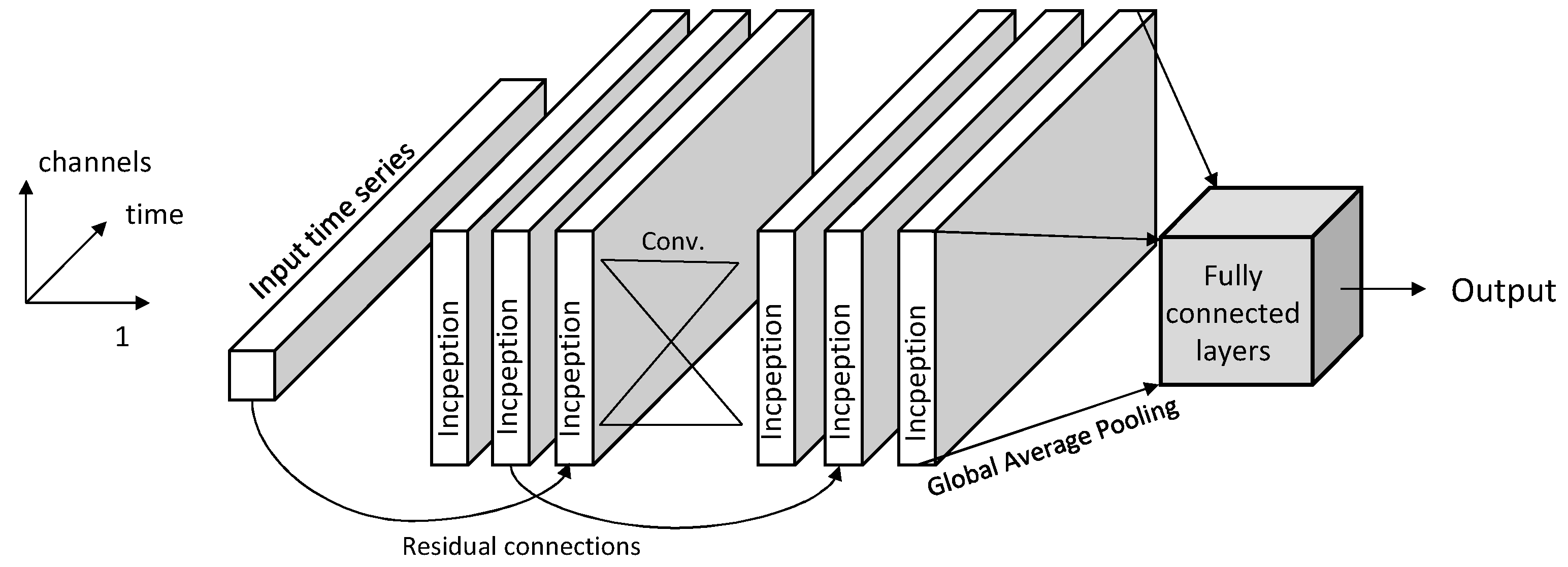
This study draws inspiration from the inception-based architecture presented in [11], as well as successful convolution-based approaches. Furthermore, the reweight mechanism that was used in the literature drives us to include such a component in our proposed methodologies. An inception-based framework was created that is easily parameterized and adjusted to sensor-based datasets with very good performance, as we demonstrate herein. More specifically, we developed two models that improve upon the previously proposed inception module, making it more appropriate for smaller datasets and reducing the risk of overfitting by reducing the number of parameters while still capturing hierarchical dependencies. Additionally, the models employ squeeze and excitation techniques to reweight the convoluted channels based on the information they contain, resulting in improved performance. Finally, a previously unused dataset was used to validate the models’ effectiveness, combined with a well-established benchmark dataset.

3. Materials and Methods

In this section, the foundations are set in order to present how the proposed models function, the datasets that were utilized in order to evaluate the approaches, and the preprocessing pipeline that was followed.

3.1. Datasets

In this chapter, the two datasets that were used are described, along with their characteristics. The datasets are the well-known benchmark Daphnet dataset and a newly introduced dataset of medium size [12]. In

Table 1. Comparison of the datasets.

Parameter	Daphnet	IMU
Subjects	10	35
Distribution	7 males, 5 females	19 males, 16 females
No. of Sensors	3	1
Placement	Shank, lower back, thigh	Leg
Readings	Accelerometer	Accelerometer, gyroscope
Tests Conducted	3	3 (not all subjects)
Annotation	Video review	Video review
Features	9 signals	6 signals

, a comparison between the individual characteristics of each dataset is presented. Analysis revealed that the two datasets possess distinct characteristics that present challenges in accurately detecting episodes of freezing of gait. Using both datasets in combination offers a comprehensive approach to test and evaluate the performance of a model.

3.1.1. Daphnet

The Daphnet dataset, which was created through a collaboration between the Tel Aviv Sourasky Medical Center and the Wearable Computing Lab of ETH Zurich, is an excellent resource for researchers in this field. It provides a comprehensive collection of data from PD patients, including measurements of movement and other clinical data [13].

The aim of the project was to develop a system that could detect FoG episodes and provide auditory notifications to patients. The dataset was created by collecting data from 10 PD patients (7 males and 3 females). The data collection process involved three stages: walking in a straight line with several turns, normal walking with 360-degree turns with were included, and conducting daily activities.

The total duration of the experiment was approximately 30 min per patient. During data collection, each subject wore 3 sensors: on their shank, their lower back, and their thigh. These sensors transmitted accelerometer measurements at a frequency of 64 Hz, resulting in a 9-signal dataset. The dataset annotated was done through video review of all tasks by specialized medical personnel.

The dataset contains three types of labels. The first type pertains to data that were gathered from patients before any experiments were conducted, during which the subjects were in a standing-by position. We excluded these examples from our approach. The remaining labels correspond to instances of freezing of gait (FoG) and normal walking.

Regarding the analysis of the dataset, we concatenated the data of all subjects together, excluding the “idle” samples. The results for each feature are depicted in the

Table 2. Descriptive statistics of Daphnet.

Measure	ankle(hr)	ankle(v)	ankle(hl)	thigh(hr)	thigh(v)	thigh(hl)	trunk(hr)	trunk(v)	trunk(hl)
mean	$-104.05$	995.17	244.86	3.15	765.19	145.24	56.65	957.72	18.42
std	577.2	363.63	322.75	567.22	369.66	275.53	202.38	196.73	218.05
max	27,651.0	31,493.0	29,437.0	22,596.0	22,596.0	22,596.0	6707.0	24,298.0	4300.0
min	−31,234.0	−32,255.0	−31,487.0	−21,846.0	−29,673.0	−23,908.0	−3951.0	$-1323.0$	$-4242.0$
kurtosis	305.4	1084.88	1447.31	77.16	271.94	1121.437	6.49	369.59	12.37
skewness	3.94	7.57	2.02	1.97	0.36	$-11.39$	0.14	0.90	$-0.68$

below.

The analysis revealed that out of the nine features, only two exhibited a symmetric distribution, while the remaining features are either slightly or extremely skewed. Furthermore, most features demonstrate extremely large kurtosis values, indicating a leptokurtic distribution and a higher likelihood of outliers. These observations suggest that the features do not conform to a normal distribution, making it more challenging for a model to learn from them. To assess the stationarity of each time series, an augmented Dickey–Fuller (ADF) test was conducted [19], which is a common way to test for a unit root in time-series data [20]. The null hypothesis of the ADF test assumes that the time series has a unit root, implying that it is non-stationary. The alternative hypothesis, on the other hand, assumes that the time series is stationary, indicating the absence of a trend. According to the results, the time series are stationary, which is expected in the context of monitoring walking patterns using accelerometers.

3.1.2. IMU Dataset

A relatively unused dataset was introduced in [12]. The dataset contains data from 35 patients diagnosed with Parkinson’s disease. The sample consists of 16 females and 19 males. The sensor used was an inertial measuring unit (IMU) that transmitted accelerometer and gyroscope data of the 3 axes using a frequency of 64 Hz, producing a total of 6 signals.

In order to evaluate their straddle, the subjects had to conduct several 360-degree turns, with a different rotation each time; the duration of this test was 2 min. Most of the patients completed 3 sessions, while 12 of them completed 2 sessions, and 8 of them only completed 1 session. For each session, the total time of FoG was provided, along with other metrics, including H&Y score. Additionally, except the IMU measurements, video recordings of each test are provided. Based on these recordings, specialized medical professionals were able to annotate the data of each subject and identify FoG episodes.

An analysis comparable to that performed on the Daphnet dataset was carried out to gain a deeper understanding of the characteristics of the IMU dataset.

An analysis comparable to that performed on the Daphnet dataset was carried out to gain a deeper understanding of the characteristics of the IMU dataset. This analysis (as shown in

Table 3. Descriptive statistics of the IMU dataset.

Measure	ACC ML	ACC AP	ACC SI	GYR ML	GYR AP	GYR SI
mean	0.03	$-0.25$	0.98	$-3.76$	0.74	$-1.57$
std	0.56	0.42	0.33	35.01	41.33	128.96
max	8.56	8.08	8.09	805.75	657.2	1149.8
min	$-8.56$	$-8.76$	$-7.21$	$-832.83$	$-337.26$	$-1039.65$
kurtosis	8	8	8	8	8	8
skewness	2.83	2.83	2.83	2.83	2.83	2.83

) included the computation of statistical measures such as mean, standard deviation, minimum, and maximum values, among others. Additionally, an augmented Dickey–Fuller test was conducted to determine the stationarity of the time series.

Similar to the Daphnet dataset, analysis of the IMU dataset revealed that the skewness and kurtosis of the 6 features indicate a deviation from the normal distribution. Additionally, all features exhibited a leptokurtic distribution. As in Daphnet, the ADF test revealed that all features were stationary, which is expected, considering the nature of the data. It is noteworthy that some measurements showed a small range between the minimum and maximum values, which can be attributed to the quality and limitations of the sensor.

It is worth noting that if the ADF test had revealed non-stationarity in the features, certain preprocessing methods such as differencing may have been required to properly fit any model and ensure the validity of the results [21]. Additionally, to account for fluctuations and normalize the examples, normalization techniques such as batch normalization would have been incorporated into the proposed models.

3.2. Preprocessing

3.2.1. Oversampling Methods

Due to the nature of the selected datasets, there was an imbalance, which is a common issue when dealing with real-world data. Oversampling and undersampling are common techniques used to address this issue [22,23].

In this study, oversampling was utilized, as it has been shown to be more effective than undersampling in many cases of binary classification [24]. The literature provides several sophisticated oversampling techniques, particularly for signal processing. In [22], such methods were discussed and tested using a CNN to classify the state of Parkinson’s patients. The proposed methods included rotation, permutation, time wrapping, scaling, cropping, and magnitude wrapping. Among the mentioned methods, a combination of signal rotation and permutation achieved the most significant improvement for the task. A similar data augmentation technique, signal inversion, was also employed in [5].

To measure their effects and improve the classification accuracy of our networks, we applied permutation of the window and rotation of the original signal in this work.

Permutation: First, the signal is segmented into N windows of equal length, where N depends on the length of the dataset (see Section 3.2.2); then, the window is divided into Z subwindows. In this study, 5 sub-windows were used, which were randomly shuffled and concatenated together, recreating the initial representation. By introducing a random factor to the order of the data, we aimed to generate diverse samples from the original dataset, simulating examples from the minority class that may not have been captured in the original dataset.

Rotation or Inversion: The signal in this case is rotated, according to a linear transformation. More specifically, a 180-degree turn was applied in the x axis for each sensor. The method of rotating the signal helps to simulate a different scenario wherein the position and orientation of the sensors have changed but the underlying pattern or phenomenon being recorded remains unchanged. This approach has several advantages over other augmentation methods, as it still follows the “real” data distribution while providing a wider variety of examples to train on. Thus, the model can become more robust and better at handling variability during deployment.

3.2.2. Window Partitions

Window Segmentation & Overlap: In addition to data augmentation techniques, windowing is another common practice in signal processing for analysis of time-series data. By dividing the signal into overlapping windows, it is possible to extract features and patterns that are specific to different segments of the signal. In this study, the size of the window was determined based on the frequency of the recordings and the distribution of FoG episode duration, resulting in windows with lengths of 256, 196, and 128 observations corresponding to 4, 3, and 2 s at a frequency of 64 Hz, respectively. To generate more examples and extract as much information as possible, an amount of overlap was used. The window size was rolled by a constant value of 4, 16, or 96 depending on the test. The label for each window was determined by counting the individual labels and retaining the most frequent one. Finally, the resulting windows were used for feature extraction or the application of deep learning methodologies such as convolutional operations.

3.3. Model Architecture

3.3.1. Components

In this section, the building components that were used in order to construct the proposed models are discussed and explained in order to highlight their function.

Inception module: Both proposed models, InSEption and LN-Inception, are inspired by the InceptionTime model of Fawaz et al. [25]. The architecture is depicted in Figure 1 and Figure 2. Generally, the purpose of this model is to apply parallel convolutions for classification of time series data. The architecture used is quite similar to Inception-v4; the core of the network is the inception module. This consists of a bottleneck layer, 3 parallel convolutional layers, and 1 max pooling plus a bottleneck convolutional layer. Each layer accomplishes a different task. The bottleneck layer reduces the dimensions of the original time series by applying a 1D convolution of a number of filters with a stride of 1 so that the overall model becomes simpler and probably less prone to overfitting. The three parallel 1D convolutions that follow the Bottleneck layer are able to extract several features from different levels. Additionally, the max pooling with the Convolutional layer, similar to the bottleneck, is responsible for making the model more stable and less susceptible to noise. Finally, all outputs are concatenated together, creating a new representation of the original multivariate time series. This representation is normalized via a batch normalization stage, and “ReLU” is applied in the end.

Residual Connections: Another characteristic that improves the performance of models and secures the constant gradient flow is the shortcut module. This module is applied to every other stacked inception module and transforms its input. After applying these inception procedures, the final representation of the multivariate time series is reduced by global average pooling, and the output is then passed through several fully connected layers. Finally, “softmax” or “sigmoid” activations are utilized, depending on the classes that have to be predicted.

Squeeze and Excitation module: The squeeze and excitation module was introduced by Hu et al. [26] in an attempt to enhance the representation ability of the networks by incorporating the relations of the channels into a final multidimensional matrix via weighting. More precisely, this particular module has two parts: (a) the squeeze part and (b) the excitation part. The first section is tasked with aggregating the input across channels to create a general depiction of the features. Then, the excitation block is able to reweight the available information in order to emphasize more descriptive channels. The SE blocks can be stacked together to extract and recalibrate features from different hierarchies. The architecture consists of a global average pooling layer that is able to extract information throughout the channels. Then, in order to reduce the dimensions of the input and the complexity of the calculations, a bottleneck layer is applied using "ReLU" activation. This layer is not fixed; instead, its size is determined empirically to increase or decrease the squeeze operation. The authors suggest a ratio of 16, meaning that the original number of channels is divided by 16 to determine the number of neurons in the bottleneck stage. Finally, reweighting is achieved through a fully connected layer using “sigmoid” activation, and a rescaling operation follows to restore the dimensions of the input. This block can be applied to inception networks. The SE block can be applied either after the inception module or immediately after the residual connection.

3.3.2. Proposed Models

The general belief that is supported by research evidence indicates that the an inception network is the state of the art for complex datasets with multiple dimensions, such as images or videos. In [11,25], the authors showed that an inception network can be successfully applied to time-series data. The methodologies used in the literature consist of an inception network with 3 parallel layers of convolutions. To the best of our knowledge, except these two implementations, there are no other examples of implementations that use this method or a similar method for the selected datasets.

Light-Normalized Inception: The first proposed model is a lighter inception model with heavy regularization procedures, namely LN-Inception. More specifically, the light inception module consists of only 2 parallel convolutional operations added to the max pool plus bottleneck stage in an attempt to simplify the network in order to make it faster and less prone to overfitting for small datasets such as Daphnet. The modified Inception module is depicted in Figure 3. A batch normalization layer is used first on the input to keep the mean at 0 and the standard deviation at 1. The residual connection module remains as proposed in the original literature. Finally, after the inception operations, a dropout layer follows with a 50% rate, similarly to that proposed in [4]. This results in an enhanced ability to precisely learn more the dependencies of the created features, mitigating the threat of overfitting. Next, instead of global average pooling, an average max pooling layer is used. The idea is that we want to extract the most prominent features after the inception layers in order to not dilute and normalize the result of the transformation. Finally, several dense layers accompanied by dropout are added to the network to process the embeddings for the final classification. These layers use “ReLU” activation.

InSEption: The second proposed network utilizes the benefits of the inception module with the addition of squeeze and excitation blocks. These blocks are able to reweight the multichannel outputs of the convolutions and isolate the most beneficial features, even further enhancing the performance of an inception network. First, the inception module was modified to use filter sizes of 5 and 7, also incorporating a bottleneck layer. The module is depicted in Figure 4. The squeeze and excitation block remained the same, along with the residual connection operation; these two modules are described in Section 3.3.1. More precisely, after each inception module, a squeeze and excitation stage follows. Then the residuals are incorporated in the embedding after every other layer. There, an additional Squeeze and excitation block is applied. After these operations, the feature extraction stage of the network is concluded by again applying an SE block to determine the final weights of the vector, followed by a dropout layer of 50% and a global average pooling layer to aggregate the channels into a single channel. Finally, similarly to the LN inception, a number of dense layers with dropout is used to produce the final probabilities using a “sigmoid” activation.

In addition to their improved performance, both proposed networks were designed in a modular manner to allow for easy modification of their hyperparameters. This flexible design makes it possible to tailor the networks to specific requirements. Therefore, no specific structure is described in this part; instead, the overall strategy of block sequences are examined in this study. Finally, this modular approach also allows for future improvements and updates to the models as new research emerges.

3.4. Experimental Setup

3.4.1. Hardware and Software Specifications

All experiments required access to a server, which was made available by the university’s laboratory. The specifications of this computer were an Intel i9-12900k, 64 GB of RAM, and an NVIDIA GeForce RTX 3090 graphics card. In addition, all the neural networks were developed using Keras [27], a Library that provides an API to Tensorflow, which allows for easier and simpler development of neural networks, better understanding of possible errors, detailed documentation, and a large community for support. In addition, other libraries were used, such as Scikit Learn for preprocessing tasks and error metrics [28] and NumPy for linear algebra calculations [29].

3.4.2. Comparative Methods

In order to compare our inception-based models, we employed a similar method that was trained on the Daphnet dataset and presented in [11], namely iSPLInception.

The architecture of the model is described as follows. First, the data were passed through a batch normalization layer; then, several inception modules with residual connections were applied. Finally, the output was transformed through a dense layer of “ReLU” activations, followed by global average pooling to aggregate the channels. The final layer depends on the application. For the case of the Daphnet dataset, “softmax” activation was used.

It is worth noting that this model’s inception module differs than that of the blocks proposed in this case. More specifically, they use 1 × 1, 1 × 3, and 1 × 5 parallel convolutions, with a bottleneck layer applied before, while the max pooling plus bottleneck application is the same.

Furthermore, the authors employed a specific train–validation–test data split. The data partition was implemented as follows. For testing purposes, only the S2-1, S4-1, and S5-2 were used. For validation, the S2-2, S3-3, and S5-1 were utilized, and the model was trained on the remaining sub datasets. For this case, a 3 s (192 examples) window was used with 50% overlap (96 examples). Finally, out of 3 available classes of the dataset, namely, inactivity, FoG episodes, and normal walking, the latter two were retained, and all the observations of the first type were discarded.

The class distribution for each part of the split was as follows: 8.7% of the data were freeze examples in the training set, 7.20% in the test set, and 16% in the validation set.

To facilitate the comparison between the proposed methodologies, two additional benchmark models were developed. The first model is a custom CNN architecture consisting of six consecutive convolutional layers with a ReLU activation function. The first two layers have a filter size of 7, the next layer has a filter size of 5, and the last layer has a filter size of 3. No pooling was performed between the convolutions due to the limited dimensions of the original data. The model uses a global max pooling stage for feature selection extraction of the most prominent features. The last five layers of the model are composed of dense and dropout neurons to fine tune the features and predict the final sample type. The second benchmark approach is a custom LSTM architecture. Similar to the CNN architecture, this model has six LSTM layers, followed by the same sequence of five dense and dropout layers as in the CNN architecture. The benchmark models were designed with a similar architecture as that of the proposed model to ensure a fair comparison.

4. Results

4.1. Performance of the Models on the Daphnet Dataset

As mentioned before, the particular split was unbalanced; thus, in order to enhance the learning ability of the model, an oversampling method was employed only in the training phase. Two ways of oversampling were selected: one using signal rotations by 90 degrees and another using signal permutations. The amount of examples generated from each method was set following a cumulative strategy; examples of the minority class are generated until they reach 20% using signal rotations and, an additional 10% is added using permutation. Overall, the minority class of the datasets reaches 30%. This procedure was only applied to the training dataset and not the test and validation sets.

The configurations of the two proposed models were determined after several runs based on empirical evaluation using the proposed metrics and are illustrated in

Table 4. Configuration of InSEption.

Parameter	InSEption	LN-Inception
Inception layers	6	6
Dense layers	5	5
Residual connections	Yes	Yes
Bottleneck	Yes	No
SE blocks	Yes	No
Batch size	128	64
Learning rate	0.0001	0.0001
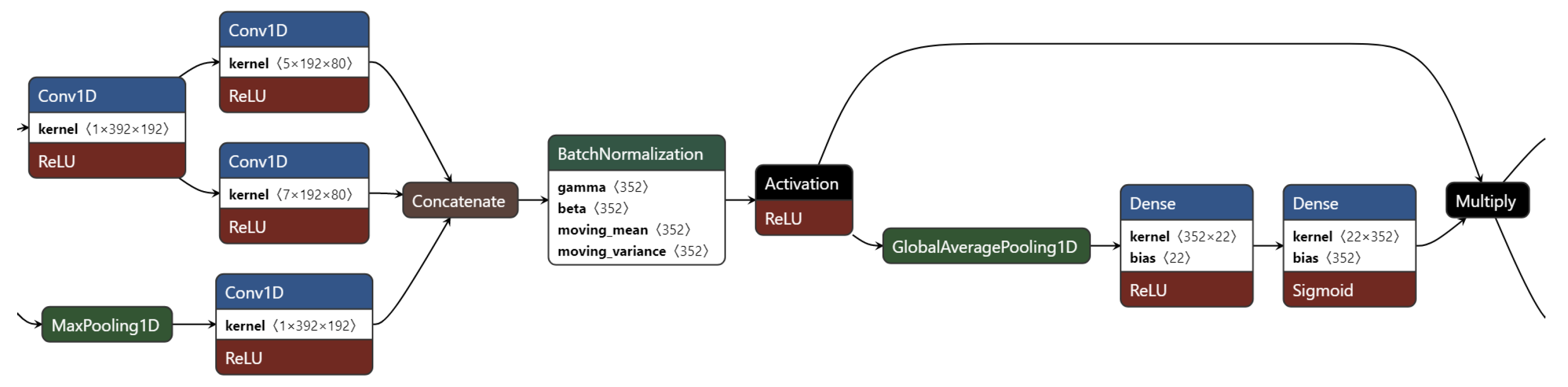
Dropout rate	0.25	0.25

. Regarding the InSEption model, the framework and modules described in the previous section were used. More precisely, the final architecture consisted of six inception layers with the squeeze and excitation add-on followed by five dense to refine the information extracted from the convolutions. This network is quite deep and complex, which is needed to extract all useful information from all the different patient datasets. The loss function used was binary cross entropy, which is the most common function for binary classification purposes. The batch size for training of the network was 128, with a learning rate of 0.0001 utilizing the Adam optimizer and its momentum adjustments. For the later dense layers, the amount of dropout was set to 25%. Finally, to avoid overfitting, early stopping was used, measuring the error of the validation set and stopping the training phase when 70 consecutive epochs did not result in any improvement in loss reduction.

The most significant parts of the InSEption network, the inception module and its connection to the squeeze and excitation block, are shown in Figure 5.

The parameters defined in the LN-Inception model are quite similar to InSEption after being validated by a series of experiments; again, six inception layers were used with 100, 80, 60, 40, 20, and 8 filters. Another five dense layers were added after, with 128, 64, 32, 16, and 8 neurons, respectively. The learning rate was 0.0001, and the dropout for the dense section of the network was 0.25. Finally, residual connections were included, but the initial bottleneck stage was excluded. The configuration is summed up in Table 4. For model training, the batch size was set to 64, along with 5000 epochs, with early stopping after 70 epochs.

The CNN benchmark model and the LSTM model have similar configurations. The CNN layers in both models had sizes of 100-80-60-40-20-8, while the dense layers were 128-64-32-8-1. The batch size for the CNN model was 128, and the learning and dropout rates were set to 0.0001 and 0.25, respectively. The LSTM model had LSTM layers with sizes of 256-128-64-32-16-8 using a “tanh” activation function, and the batch size was set to 64. Both architectures are shown in

Table 5. Configuration of Daphnet benchmark models.

Parameter	Custom CNN	Custom LSTM
CNN or LSTM layers	6	6
Dense layers	5	5
Batch size	128	64
Learning rate	0.0001	0.0001
Dropout rate	0.25	0.25

.

Regarding the results of the proposed models, F1 score was used as in the benchmark paper. The metrics were set up in the “micro” setting, which is similar to accuracy. However, accuracy for imbalanced datasets is not a suitable metric due to the increased weight that allocates to the majority class. Nevertheless, in order to compare our models with the particular inception-based model, this was necessary.

Comparing our methodologies with the existing method, it is evident that both Inception modifications perform better than the benchmark. In terms of accuracy or micro F1 score, the InSEption model outperforms the other two models 0.5%. However, the real improvement in performance is in terms of the macro F1 score, for which the proposed models reach 71% and 67%, meaning that they outperform the benchmark by 6% and 2%, respectively. Furthermore, in terms of precision and recall, the iSPLInception model fails to perform better than the proposed models. For the precision, which indicates the ability to retrieve relevant instances, the difference is 2% for the InSEption method, while for the recall, which measures the fraction of the total relevant items retrieved, there is a significant improvement by 5% when utilizing the InSEption network. Additionally, both benchmarks fail to be comparable with the inception-based models in terms of macro F1, precision, and recall, while in terms of micro F1 or accuracy, their results are closer to the best. However, due to the imbalances of the data, accuracy is not suitable to measure the performance, which we expect to be quite high. Finally, the CNN model seems to perform better than the LSTM model, reinforcing our initial strategy, which involves the development of an approach based on convolutions. The complete performance of the models can be found in

Table 6. Literature comparison of inception neural networks.

Metric	Custom CNN	Custom LSTM	iSPLInception [11]	LN-Inception	InSEption
Micro F1	92.82%	91.3%	93.52%	93.56%	94%
Macro F1	56%	53%	65%	67%	71%
Precision	74%	58%	79%	80%	81%
Recall	54%	53%	61%	62%	66%

.

In conclusion, the impact of normalization, squeeze and excitation, and oversampling using more sophisticated and domain-specific methods is quite significant for this split. However, in order for these methods to perform even better, larger datasets are required.

4.2. Performance of the Models on the IMU Dataset

For comparison and evaluation purposes, a new dataset was utilized [12]. The preprocessing procedure used was similar to that applied in the previous cases. The dates were concatenated into 2-second windows with an overlap of 16 observations in order to create enough examples from each patient. This process was repeated for each patient. The labels were generated again based on the most observed label in each segment. Finally, the datasets were concatenated together to create a single dataset.

For cross validation, a five-KFold was selected using the stratified KFold method to ensure that the proportions of each class were maintained in the subdatasets. This allowed for five different training and validation procedures to be conducted, with a more conventional split of 80% for training and validation and 20% for testing. Out of the 80% that was used for non-testing purposes, 10% comprised the validation set. The performance of the model was evaluated using three common metrics: specificity, sensitivity, and macro F1. These metrics provided insight into the model’s ability to correctly identify instances of each class and the overall balance between precision and recall.

Initially, tests were run on the imbalanced dataset without implementing any balancing techniques; however, the results were not up to the desired level of accuracy. To address this issue, additional samples were created specifically for training purposes using the methods described in Section 4. The inverse signal method was used to generate samples until the imbalanced class reached 25%, and an additional 10% was created using the permutation method. The application of these techniques greatly improved the metrics and elevated the accuracy of the network’s predictions. It is worth noting that the oversampling methods were only applied during training.

Again, as in the other experiments, the framework remained the same. The final architecture of the InSEption network was identical to that used in the iSPLInception comparison. The specific parameters are illustrated in

Table 7. Configuration of inception-based models.

Parameter	InSEption	LN-Inception
Inception layers	6	6
Inception dimensions	120-100-80-60-40-20	120-100-80-60-40-20
Dense layers	5	5
Dense layer dimensions	128-64-32-16-8-1	128-64-32-16-8-1
Validation split	0.1	0.1
Residual connections	Yes	Yes
Bottleneck	Yes	No
SE blocks	Yes	No
Batch size	32	32
Learning rate	0.0001	0.0001
Dropout rate	0.15	0.15

. The only differences are the dropout rate and the batch size, which are 15% and 32 in both networks, respectively. Other than that, both the network layers and size were the same. All the parameters were selected based on several experiments and their results.

The parameters used in the LN-Inception model were kept the same as those used in the InSEption model. However, the practical difference between the two networks lies in the absence of bottleneck and squeeze and excitation blocks in the LN-Inception model. This change in the architecture is intended to result in a simplified model that is still capable of producing high-quality results.

The architecture of the benchmark models was kept the same as in the previous experiment; the only changes were the batch size, which was set to 32, and the dropout rate, which was 15%. The overall architecture and hyperparameters can be found in

Table 8. Configuration of IMU benchmark models.

Parameter	Custom CNN	Custom LSTM
CNN/LSTM layers	6	6
CNN/LSTM dimensions	120-100-80-60-40-20	256-128-64-32-16-8
Dense layers	4	4
Dense layer dimensions	128-64-32-8	128-64-32-8
Validation split	0.1	0.1
Residual connections	No	No
Bottleneck	No	No
SE blocks	No	No
Batch size	32	32
Learning rate	0.0001	0.0001
Dropout rate	0.15	0.15

. In terms of evaluation metrics, we decided to expand beyond the sensitivity, specificity, and F1 score that were used in previous tests, since there were no models for comparison. Thus, we included two additional metrics in our analysis: the area under the curve and geometric mean. These metrics provide a more comprehensive picture of the model’s performance by taking into account the results of the confusion matrix in settings other than the usual F1 score [30,31]. Moreover, for the geometric mean, we substituted the true positive and true negative values with their success rates to improve interpretability. This substitution is equivalent to using sensitivity and specificity, and it ensures that the results are bound between 0 and 1, with 1 indicating the best performance; this approach was introduced in [32,33]. Regarding the results of the two models for this dataset, the InSEption module performs better than LN-Inception by a slight margin. More specifically, in terms of sensitivity, the difference for the first model is 1%, although in terms of specificity, both scored the same. The F1 and AUC scores indicate that, again, the squeeze and excitation blocks were beneficial, with a 0.3% and 0.5% difference against the LN-Inception, respectively. The scores that are shown in

Table 9. Results of the proposed neural networks.

Metric	Custom CNN	Custom LSTM	LN-Inception	InSEption
Sensitivity	97%	97%	97%	98%
Specificity	96%	97%	99%	99%
Macro-F1	92%	93%	96.9%	97.2%
Geometric mean	96.49%	97.0%	98.0%	98.49%
AUC	96.47%	96.9%	98.1%	98.6%

are the means of the 5K cross validation procedures that were conducted.

Compared to the benchmark models, the two proposed models show a significant improvement in terms of macro F1 score, with increases in sensitivity, specificity, geometric mean, and AUC between 1 and 2%, depending on the metric. Overall, the results on this dataset suggest that it is easier for a model to correctly predict examples, possibly due to the higher number of positive class examples compared to the Daphnet dataset.

In conclusion, the proposed methods have proven to be highly effective in classifying time-series data, particularly in detecting freezing-of-gait (FoG) episodes. The results show that the models are capable of accurately identifying both classes with high F1 and AUC scores, demonstrating their ability to effectively learn patterns and distinguish between FoG and normal walking patterns. Furthermore, the oversampling techniques employed to balance the dataset only during training were proven to be effective, as they did not compromise the model’s ability to predict the majority class, instead improving its ability to detect the minority class. During the prediction stage, the class distribution remained similar to the original dataset, with approximately 18% of instances classified as FoG and 82% classified as normal. These results highlight the strength of the proposed models and suggest that they could be effectively utilized in real-world applications for monitoring and detection of FoG episodes in Parkinson’s disease patients.

5. Discussion and Future Work

The aim of this work was to explore the potential of various deep learning architectures for prediction of episodes of freezing of gait (FoG), a debilitating symptom that significantly affects the quality of life of Parkinson’s disease (PD) patients. The early detection and classification of FoG episodes can aid practitioners in understanding the symptoms of each patient and in developing more effective strategies to treat the disease.

To achieve this goal, two inception-based models were introduced. The first model is named LN-Inception, and it is a simpler version of the original inception network for time-series classification [25]. Practically, the number of parallel convolutions was reduced, and the normalization levels increased. The second proposed methodology is the InSEption network, which, with the exception of the inception modules, integrates squeeze and excitation blocks after each convolutional stage.

In order to evaluate the effectiveness of the proposed models, the Daphnet dataset was utilized, and results were compared to existing literature, specifically the iSPLInception network, which is the only inception network that has been used with this dataset. The findings indicate that both proposed models surpassed the state-of-the-art performance in terms of all metrics that were used in [11]. The most significant improvement was observed in the macro F1 score, for which the models demonstrated an improvement of 2% and 6%, with the InSEption network exhibiting the highest performance.

The last experiments were carried out utilizing an additional dataset related to FoG (freezing of gait) episodes, which was collected from an IMU (inertial measuring unit) sensor. This resulted in six features for each participant. It is important to note that this dataset is relatively new, and no established benchmarks exist, making this study unique and potentially contributing to the creation of benchmark standards for future research in this area. For the evaluation, data for each patient were organized similarly to the Daphnet dataset.

Regarding the results, it can be observed that both models performed exceptionally well, achieving high scores for both the F1 and AUC metrics, with scores of 96.9% and 97.2% for F1 and 98.1% and 98.6% for AUC, respectively. These scores were notably higher than those of the two custom models that were developed for comparison. Furthermore, both had sensitivity, specificity, and GM scores over 97%. The reason we utilized AUC and GM as evaluation metrics in this setting is that there is no established benchmark in the literature for comparison that specifies the metrics to be used. In addition, the use of these metrics allowed us to further validate the effectiveness of our models. The results demonstrated that our proposed models outperformed created custom benchmark models in terms of these metrics. The best-performing network was, again, InSEption. In order for these results to be achieved, the abovementioned oversampling methods were employed.

In summary, this study highlights the benefits of using the inception mechanism to extract multiple hierarchical features from signal data. Additionally, the positive impact of incorporating squeeze and excitation blocks and problem-specific oversampling methods further enhances the overall performance of the proposed models. The results of this study demonstrate the potential of the inception-based deep learning architectures for prediction of FoG episodes in PD patients and their suitability for integration into wearable IoT devices for real-time monitoring and early intervention. Additionally, due to the different features of the two dataset and their satisfactory performances, the inception methodologies constitute a potentially very efficient way to treat signal or sensor datasets.

In regard to future research, it may be worthwhile to investigate the use of time-dependent modules, such as gated recurrent units (GRUs), long short-term memory (LSTM) networks, or attention mechanisms, to further exploit the features extracted from the convolutional layers and incorporate additional temporal information, as has been successfully done in previous studies [5,9]. Additionally, it would be valuable to evaluate the proposed methodologies on larger Parkinson’s-related datasets, such as mPower, or on other activity recognition datasets in order to determine their generalizability and efficacy across a wider range of tasks. Furthermore, in addition to the proposed variations, transfer learning could be explored as a potential approach, building upon the methods introduced in previous works [8,10]. With transfer learning, the proposed models could be trained extensively on a large dataset, then fine-tuned for predictions on another dataset, potentially incorporating more generalized knowledge and avoiding overfitting. These avenues of research could help to further validate the potential of these models for use in wearable IoT devices for real-time monitoring and early intervention in conditions such as freezing of gait (FoG).

References

1. Pardoel, S.; Kofman, J.; Nantel, J.; Lemaire, E.D. Wearable-Sensor-Based Detection and Prediction of Freezing of Gait in Parkinson’s Disease: A Review. Sensors 2019, 19, 5141. [Google Scholar] [CrossRef]
2. Myszczynska, M.A.; Ojamies, P.N.; Lacoste, A.M.B.; Neil, D.; Saffari, A.; Mead, R.; Hautbergue, G.M.; Holbrook, J.D.; Ferraiuolo, L. Applications of Machine Learning to Diagnosis and Treatment of Neurodegenerative Diseases. Nat. Rev. Neurol. 2020, 16, 440–456. [Google Scholar] [CrossRef] [PubMed]
3. Giannakopoulou, K.-M.; Roussaki, I.; Demestichas, K. Internet of Things Technologies and Machine Learning Methods for Parkinson’s Disease Diagnosis, Monitoring and Management: A Systematic Review. Sensors 2022, 22, 1799. [Google Scholar] [CrossRef] [PubMed]
4. Bikias, T.; Iakovakis, D.; Hadjidimitriou, S.; Charisis, V.; Hadjileontiadis, L.J. DeepFoG: An IMU-Based Detection of Freezing of Gait Episodes in Parkinson’s Disease Patients via Deep Learning. Front. Robot AI 2021, 8, 537384. [Google Scholar] [CrossRef] [PubMed]
5. Li, B.; Yao, Z.; Wang, J.; Wang, S.; Yang, X.; Sun, Y. Improved Deep Learning Technique to Detect Freezing of Gait in Parkinson’s Disease Based on Wearable Sensors. Electronics 2020, 9, 1919. [Google Scholar] [CrossRef]
6. Tăuţan, A.-M.; Andrei, A.-G.; Ionescu, B. Freezing of Gait Detection for Parkinson’s Disease Patients Using Accelerometer Data: Case Study. In Proceedings of the 2020 International Conference on e-Health and Bioengineering (EHB), Iasi, Romania, 29–30 October 2020; pp. 1–4. [Google Scholar]
7. Shalin, G.; Pardoel, S.; Lemaire, E.D.; Nantel, J.; Kofman, J. Prediction and Detection of Freezing of Gait in Parkinson’s Disease from Plantar Pressure Data Using Long Short-Term Memory Neural-Networks. J. Neuroeng. Rehabil. 2021, 18, 167. [Google Scholar] [CrossRef] [PubMed]
8. Hssayeni, M.D.; Jimenez-Shahed, J.; Burack, M.A.; Ghoraani, B. Ensemble Deep Model for Continuous Estimation of Unified Parkinson’s Disease Rating Scale III. BioMed Eng. OnLine 2021, 20, 32. [Google Scholar] [CrossRef]
9. Meyer, B.M.; Tulipani, L.J.; Gurchiek, R.D.; Allen, D.A.; Adamowicz, L.; Larie, D.; Solomon, A.J.; Cheney, N.; McGinnis, R.S. Wearables and Deep Learning Classify Fall Risk From Gait in Multiple Sclerosis. IEEE J. Biomed. Health Inform. 2021, 25, 1824–1831. [Google Scholar] [CrossRef]
10. Torvi, V.G.; Bhattacharya, A.; Chakraborty, S. Deep Domain Adaptation to Predict Freezing of Gait in Patients with Parkinson’s Disease. In Proceedings of the 2018 17th IEEE International Conference on Machine Learning and Applications (ICMLA), Orlando, FL, USA, 17–20 December 2018; pp. 1001–1006. [Google Scholar]
11. Ronald, M.; Poulose, A.; Han, D.S. ISPLInception: An Inception-ResNet Deep Learning Architecture for Human Activity Recognition. IEEE Access 2021, 9, 68985–69001. [Google Scholar] [CrossRef]
12. Ribeiro De Souza, C.; Miao, R.; Ávila De Oliveira, J.; Cristina De Lima-Pardini, A.; Fragoso De Campos, D.; Silva-Batista, C.; Teixeira, L.; Shokur, S.; Mohamed, B.; Coelho, D.B. A Public Data Set of Videos, Inertial Measurement Unit, and Clinical Scales of Freezing of Gait in Individuals with Parkinson’s Disease during a Turning-In-Place Task. Front. Neurosci. 2022, 16, 832463. [Google Scholar] [CrossRef]
13. Bachlin, M.; Plotnik, M.; Roggen, D.; Maidan, I.; Hausdorff, J.M.; Giladi, N.; Troster, G. Wearable Assistant for Parkinson’s Disease Patients with the Freezing of Gait Symptom. IEEE Trans. Inf. Technol. Biomed. 2010, 14, 436–446. [Google Scholar] [CrossRef] [PubMed]
14. Güney, S.; Bölül, B. Daphnet Freezing Recognition with Gait Data by Using Machine Learning Algorithms. In Proceedings of the 2020 43rd International Conference on Telecommunications and Signal Processing (TSP), Milan, Italy, 7–9 July 2020; pp. 252–255. [Google Scholar]
15. Noor, M.H.M.; Nazir, A.; Wahab, M.N.A.; Ling, J.O.Y. Detection of Freezing of Gait Using Unsupervised Convolutional Denoising Autoencoder. IEEE Access 2021, 9, 115700–115709. [Google Scholar] [CrossRef]
16. Farhani, G.; Zhou, Y.; Jenkins, M.E.; Naish, M.D.; Trejos, A.L. Using Deep Learning for Task and Tremor Type Classification in People with Parkinson’s Disease. Sensors 2022, 22, 7322. [Google Scholar] [CrossRef] [PubMed]
17. Cole, B.T.; Roy, S.H.; Nawab, S.H. Detecting Freezing-of-Gait during Unscripted and Unconstrained Activity. In Proceedings of the 2011 Annual International Conference of the IEEE Engineering in Medicine and Biology Society, Boston, MA, USA, 30 August–3 September 2011; pp. 5649–5652. [Google Scholar]
18. Das, R.; Paul, S.; Mourya, G.K.; Kumar, N.; Hussain, M. Recent Trends and Practices Toward Assessment and Rehabilitation of Neurodegenerative Disorders: Insights From Human Gait. Front. Neurosci. 2022, 16, 859298. [Google Scholar] [CrossRef]
19. Dickey, D.A.; Fuller, W.A. Likelihood Ratio Statistics for Autoregressive Time Series with a Unit Root. Econometrica 1981, 49, 1057–1072. [Google Scholar] [CrossRef]
20. Weigend, A.S. Time Series Prediction: Forecasting the Future and Understanding the Past; Routledge: Oxfordshire, UK, 2018; ISBN 978-0-429-97227-0. [Google Scholar]
21. Livieris, I.E.; Pintelas, P. A Novel Multi-Step Forecasting Strategy for Enhancing Deep Learning Models’ Performance. Neural Comput & Applic. 2022, 34, 19453–19470. [Google Scholar] [CrossRef]
22. Um, T.T.; Pfister, F.M.J.; Pichler, D.; Endo, S.; Lang, M.; Hirche, S.; Fietzek, U.; Kulić, D. Data Augmentation of Wearable Sensor Data for Parkinson’s Disease Monitoring Using Convolutional Neural Networks. In Proceedings of the 19th ACM International Conference on Multimodal Interaction, Glasgow, UK, 13–17 November 2017; pp. 216–220. [Google Scholar]
23. A Review on Imbalanced Data Handling Using Undersampling and Oversampling Technique. IJRTER 2017, 3, 444–449. [CrossRef]
24. Mohammed, R.; Rawashdeh, J.; Abdullah, M. Machine Learning with Oversampling and Undersampling Techniques: Overview Study and Experimental Results. In Proceedings of the 2020 11th International Conference on Information and Communication Systems (ICICS), Irbid, Jordan, 7–9 April 2020; pp. 243–248. [Google Scholar]
25. Ismail Fawaz, H.; Lucas, B.; Forestier, G.; Pelletier, C.; Schmidt, D.F.; Weber, J.; Webb, G.I.; Idoumghar, L.; Muller, P.-A.; Petitjean, F. InceptionTime: Finding AlexNet for Time Series Classification. Data Min. Knowl. Disc. 2020, 34, 1936–1962. [Google Scholar] [CrossRef]
26. Hu, J.; Shen, L.; Sun, G. Squeeze-and-Excitation Networks. In Proceedings of the IEEE Conference on Computer Vision and Pattern Recognition, Salt Lake City, UT, USA, 18–23 June 2018; pp. 7132–7141. [Google Scholar]
27. Keras: The Python Deep Learning API. Available online: https://keras.io/ (accessed on 1 March 2023).
28. Scikit-Learn: Machine Learning in Python—Scikit-Learn 1.2.1 Documentation. Available online: https://scikit-learn.org/stable/ (accessed on 1 March 2023).
29. NumPy. Available online: https://numpy.org/ (accessed on 1 March 2023).
30. Livieris, I.E.; Kiriakidou, N.; Stavroyiannis, S.; Pintelas, P. An Advanced CNN-LSTM Model for Cryptocurrency Forecasting. Electronics 2021, 10, 287. [Google Scholar] [CrossRef]
31. Pintelas, E.; Livieris, I.E.; Pintelas, P.E. A Convolutional Autoencoder Topology for Classification in High-Dimensional Noisy Image Datasets. Sensors 2021, 21, 7731. [Google Scholar] [CrossRef]
32. Kubat, M.; Matwin, S. Addressing the Curse of Imbalanced Training Sets: One-Sided Selection. Icml 1997, 97, 197. [Google Scholar]
33. Barandela, R.; Sánchez, J.; García, V.; Rangel, E. Strategies for Learning in Class Imbalance Problems. Pattern Recognit. 2003, 36, 849–851. [Google Scholar] [CrossRef]
Figure 1. The architecture of an inception module.
Electronics 12 02088 g001
Figure 2. The architecture of InceptionTime.
Electronics 12 02088 g002
Figure 3. An overview of light inception module.
Electronics 12 02088 g003
Figure 4. An overview of the InSEption module.
Electronics 12 02088 g004
Figure 5. An overview of the InSEption layer with SE added.
Electronics 12 02088 g005