LiDAR Point Cloud Object Recognition Method via Intensity Image Compensation

Abstract

LiDAR point cloud object recognition plays an important role in robotics, remote sensing, and automatic driving. However, it is difficult to fully represent the object feature information only by using the point cloud information. To address this challenge, we proposed a point cloud object recognition method that uses intensity image compensation, which is highly descriptive and computationally efficient. First, we constructed the local reference frame for the point cloud. Second, we proposed a method to calculate the deviation angle between the normal vector and local reference frame in the local neighborhood of the point cloud. Third, we extracted the contour information of the object from the intensity image corresponding to the point cloud, carried out Discrete Fourier Transform on the distance sequence between the barycenter of the contour and each point of the contour, and took the obtained result as Discrete Fourier Transform contour feature of the object. Finally, we repeated the above steps for the existing prior data and marked the obtained results as the feature information of the corresponding object to build a model library. We can recognize an unknown object by calculating the feature information of the object to be recognized and matching the feature information with the model library. We rigorously tested the proposed method with avalanche photon diode array LiDAR data and compared the results with those of four other methods. The experimental results show that the proposed method is superior to the comparison method in terms of description and computational efficiency and that it can meet the needs of practical applications.

1. Introduction

Avalanche photon diode (APD) array LiDAR has been widely used in 3D imaging due to its extremely high photon sensitivity and picosecond time resolution [1]. LiDAR point cloud object recognition is a basic research direction of photoelectric and computer vision technology. With the development of 3D scanning technology, point cloud object recognition has been increasingly applied in 3D reconstruction [2], indoor mapping [3,4], automatic driving [5], and other fields.

In recent years, many research studies have been carried out on LiDAR point cloud object recognition. According to the technical approach, it is generally divided into two technical routes: feature matching and deep learning. Object recognition based on feature matching uses feature descriptors to represent the distribution of the object in a three-dimensional space and then realizes the recognition of the object types by matching the features between the object and the model library. One example is the signature of histograms of orientations (SHOT) proposed by Tombari et al. [6]. They divided the feature point neighborhood into a three-dimensional sphere and calculated the deviation angle histogram of the normal vector of the feature point and the normal vector of the adjacent point, using the normal deviation of each subspace to describe the feature. Zhao et al. proposed the statistic of deviation angles on subdivided space (SDASS) algorithm [7], which features a calculation method to determine the local minimum axis (LMA) and uses two spatial features to fully encode spatial information on local surfaces to improve the robustness of the algorithm with regard to changes in grid resolution. Zhao et al. proposed the histograms of point pair features (HoPPF) algorithm [8]. They divided the local point pairs of each key point into eight regions and constructed the corresponding subfeatures using the local point pair distribution of each region. Finally, the proposed HoPPF is generated by concatenating all the subfeatures into a vector. Guo et al. proposed a rotational projection statistics (RoPS) algorithm [9]. They generated the feature representation by calculating a series of statistics about the point density of multiple rotations around the local surface of each axis. The RoPS method has been shown to be highly descriptive [10]. Ge et al. proposed a key point pair feature (K–PPF) algorithm [11]. They used the method to combine the curvature adaptive and grid ISS to extract the sample points and carried out angle adaptive judgment on the sampling points to extract the key points to improve the point pair feature difference and matching accuracy.

With the development of deep learning, much research has been conducted regarding object recognition using deep learning. Object recognition based on deep learning obtains prior knowledge of object features in advance through feature calculations of a large number of sample sets. As an example, Qi et al. proposed the PointNet series network [12,13]. They used symmetric functions to aggregate features and used the maxpooling function to improve the aggregation ability of the local neighborhood descriptor. Manturana et al. proposed VoxelNet [14], which changed point cloud data into voxels and calculated features based on the grid. It dramatically improved the computation speed. Liu et al. proposed the self-contour-based transformation (SCT) method [15]. They proposed contour-aware-transformation that provides effective rotation and shift invariance. The recognition feature extraction is enhanced by capturing the contour and converting the self-contour-based frame into the intraclass-based frame. Jin et al. proposed the SectionKey method [16]. They used two kinds of information, semantic and geometric, to solve the identification problem and used the two-step semantic iterative closest point (ICP) algorithm to obtain the three-dimensional pose, which was used to align the candidate point cloud with the query framework and calculate the similarity score. In recent years, attention mechanisms and graphic-based methods have been used to make great progress in the field of computer vision. Zhao et al. proposed a point transformer with a transformer layer to ensure alignment and cardinality invariance and a point transformer layer to realize high-performance classification and segmentation [17]. Qian et al. proposed BADet [18]. They used a node representation scheme with a finite radius to construct the local neighborhood diagram of the 3D object detector.

At present, the object recognition of a LiDAR point cloud is generally performed through point cloud and information fusion (infrared and laser fusion, visible and laser fusion, etc.). Because this relies on a single information type, the recognition accuracy of point cloud information recognition is sometimes lower than that of information fusion. However, since the object recognition method based on information fusion needs to use multiple detectors to detect and image the target, it needs to carry out cross-spectral image registration before recognition, which increases the computing time of the object recognition algorithm. To address this challenge, we propose a point cloud object recognition method that uses intensity image compensation to take advantage of the APD array LiDAR feature, which can obtain the intensity image and point cloud simultaneously. First, we construct the local reference frame (LRF) for the point cloud. Second, we propose a method to calculate the deviation angle between the normal vector and the LRF in the local neighborhood of the point cloud. Third, we extract the contour information of the object from the intensity image corresponding to the point cloud, carry out the Discrete Fourier Transform (DFT) on the distance sequence between the barycenter of the contour and each point of the contour, and take the obtained result as the DFT contour feature of the object. Finally, we repeat the above steps for the existing prior data and mark the obtained results as the feature information of the corresponding object to build a model library. We can recognize an unknown object by calculating the feature information of the object to be recognized and matching the feature information with the model library. The main contributions of this paper are as follows:

(1) A novel point cloud object recognition method using intensity image compensation is proposed, which is highly descriptive and timely.

(2) The proposed method does not require cross-spectral image registration, and the obtained target intensity information is used to enrich the feature representation of point clouds and improve the accuracy of object recognition.

The rest of this paper is structured as follows: in Section 2, we discuss the details of the proposed method and give the theoretical analysis. In Section 3, we conduct experimental tests based on APD array LiDAR data and give the experimental results. Section 4 is where we present the conclusion and directions for future work.

2. Methods

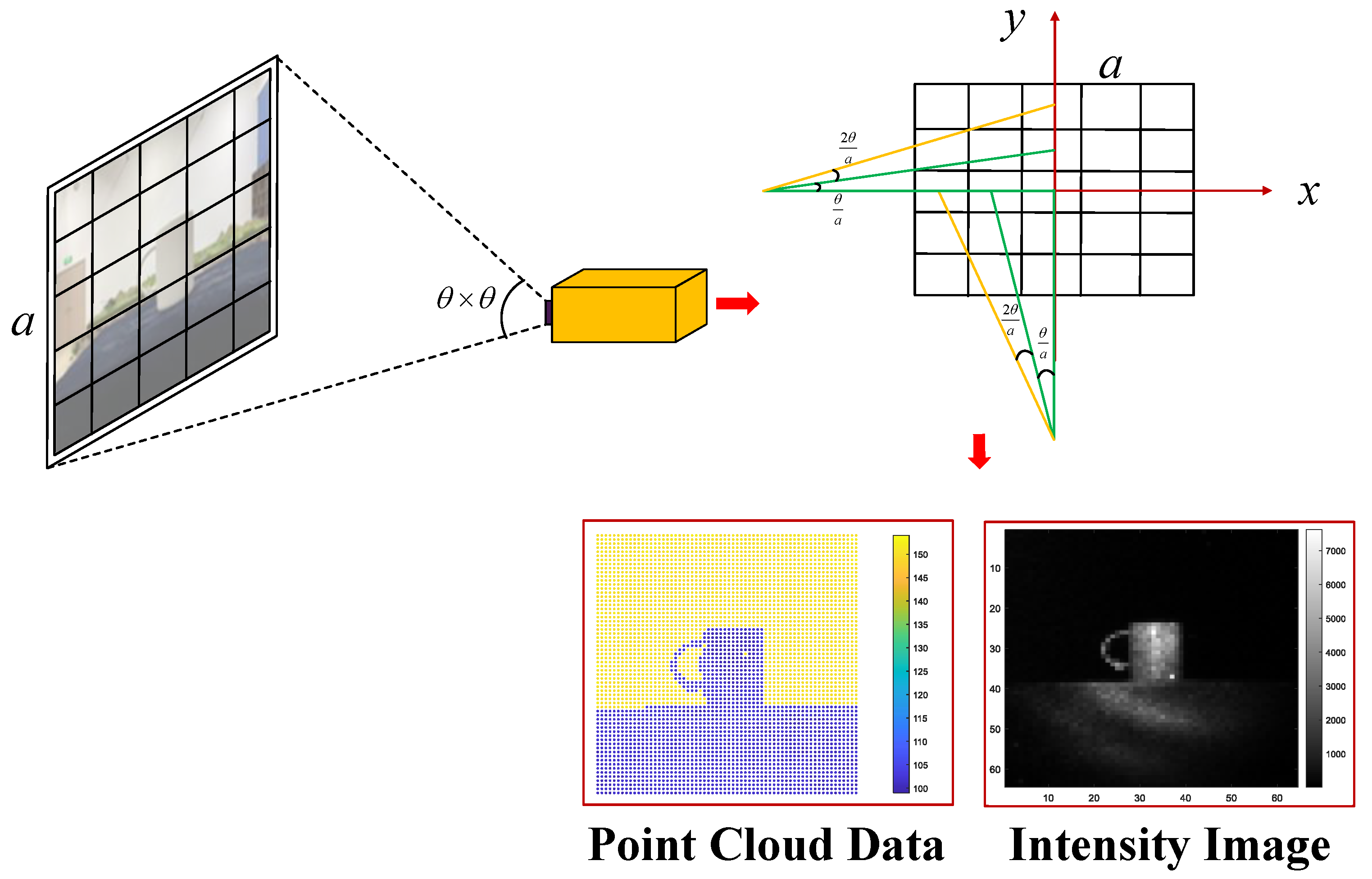
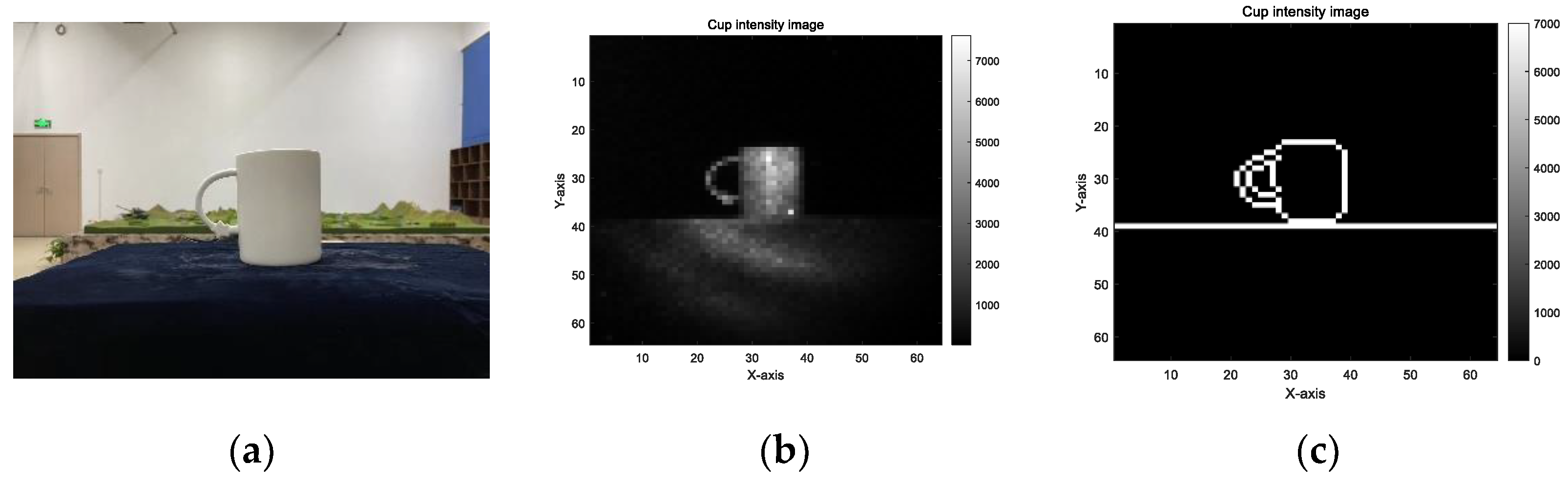
2.1. Acquisition Methods for Point Cloud and Intensity Images

The APD is a photodetector with a photoelectric effect. When the photon enters the APD, the photoelectric effect will occur, and charge carriers will be generated inside the APD. The generated carriers can obtain sufficient energy under the acceleration of the electric field to collide with the atomic lattice and produce an ionization effect. After the ionization collision effect occurs, electron hole pairs are generated. The resulting “electron hole pair” is rapidly separated by the electric field of the depletion layer inside the APD, which in turn repeats the new ionization collision effect. This process is repeated over and over again, triggering the avalanche effect of the charge carriers and generating a significant avalanche current.

Assume that the number of arrays for the APD is $a\times a$, and the beam divergence angle of LiDAR is $\theta \times \theta$. When detecting and imaging the target, $a\times a$ distance data can be obtained, denoted as $S=\left\{s_1,s_2,\cdots ,s_{a\times a}\right\}$. Each element in $S$ corresponds to each element in the APD array. The position of LiDAR is set as the coordinate origin, and the three-dimensional coordinates of each array element can be calculated by $\theta$ and $a$. The $x$- and $y$- coordinates are calculated using Equations (1) and (2):

$$x_t=\left\{\begin{array}{l}\sin \left(t\times \frac{\theta }{a}\right)\times s_t,t=-\frac{a-1}{2},1-\frac{a-1}{2},\cdots ,-1,0,1,\cdots ,\frac{a-1}{2}-1,\frac{a-1}{2},when a is odd \hfill \\ \sin \left(\frac{\theta \left(2t-1\right)}{2a}\right)\times s_t,t=-\frac{a}{2},1-\frac{a}{2},\cdots ,-1,1,\cdots ,\frac{a}{2}-1,\frac{a}{2},when a is even \hfill \end{array}\right.,$$

(1)

$$y_t=\left\{\begin{array}{l}\sin \left(t\times \frac{\theta }{a}\right)\times s_t,t=-\frac{a-1}{2},1-\frac{a-1}{2},\cdots ,-1,0,1,\cdots ,\frac{a-1}{2}-1,\frac{a-1}{2},when a is odd \hfill \\ \sin \left(\frac{\theta \left(2t-1\right)}{2a}\right)\times s_t,t=-\frac{a}{2},1-\frac{a}{2},\cdots ,-1,1,\cdots ,\frac{a}{2}-1,\frac{a}{2},when a is even \hfill \end{array}\right.,$$

(2)

The $z$-coordinate of the array element represents the distance information $s_t,t=1,2,\cdots ,a\times a$ that corresponds to the element. In summary, by combining the three-dimensional information of all points, we obtain the point cloud of the target. Since the APD is a probabilistic detection device, we can use statistical methods to obtain the intensity image of the target. By continuously detecting 20,000 frames of data for the target, the number of times each array element receives an echo signal is recorded as the intensity of that element. By assigning a pseudocolor to these intensity values, we can obtain the intensity image of the target. The schematic diagram of detection using APD array LiDAR is shown in Figure 1.

2.2. Deviation Angle Feature of Normal Vector

In this section, we illustrate the feature description process of the proposed method in detail. First, we construct the LRF for the point cloud. Second, we propose a method to calculate the deviation angle between the normal vector and the LRF in the local neighborhood of the point cloud. Third, we extract the contour information of the object from the intensity image corresponding to the point cloud, carry out the DFT on the distance sequence between the barycenter of the contour and each point of the contour, and take the obtained result as the DFT contour feature of the object. The flow chart of the proposed method is shown in Figure 2.

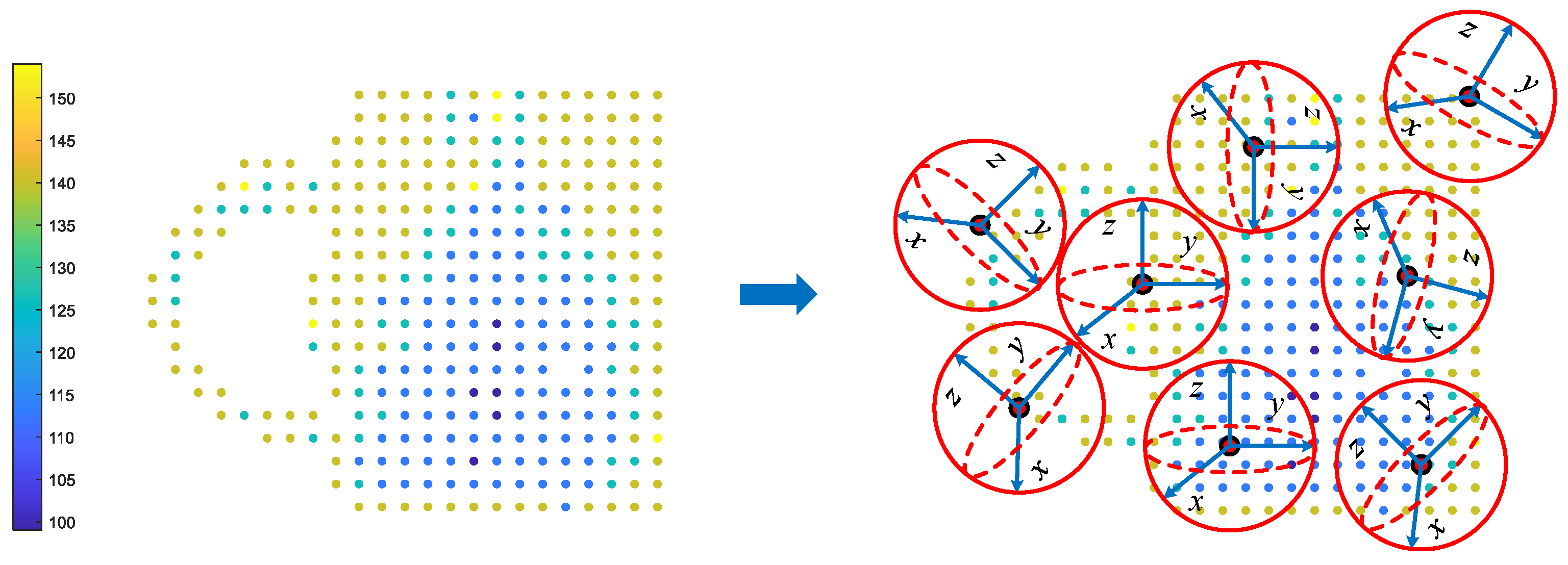
2.2.1. Construction of the LRF

Suppose the input point cloud $P=\left\{p_1,p_2,\cdot \cdot \cdot ,p_N\right\}$ contains $N$ points. In order to reduce the large amount of time needed for the amount of calculation of coordinate transformation, we constructed the LRF for $P$ during the feature calculation, as shown in Figure 3.

The LRF is an independent coordinate system separate from the global coordinate system. The primary purpose of constructing the LRF is to reduce the computational time spent on numerous coordinate transformations and to facilitate the parallel optimization of algorithms. We construct the LRF for each point by calculating the eigenvectors of their covariance matrix [6] and then project the points in the feature point neighborhood into the LRF. Taking point $P_i$ as an example, we describe the detailed steps for constructing the LRF as follows: taking a point $P_i$ in $P$, for example, suppose that the coordinate of $P_i$ is $P_i(x_{P_i},y_{P_i},z_{P_i})$ and the support radius of the feature point neighborhood is $r$. $P_{ik}(x_{k{P}_i},y_{k{P}_i},z_{k{P}_i})$ is the coordinate of the $k$th feature point neighborhood of $P_i$. Increasing the weight of the point clouds close to $P_i$, the divergence matrix of the point cloud is shown in Equation (3).

$$C=\frac{1}{{\displaystyle \sum _k(r-f_i)}}{\displaystyle \sum _k(r-f_i)(P_{ik}-P_i)}{(P_{ik}-P_i)}^T,$$

(3)

where $f_i={‖P_{ik}-P_i‖}_2$. Eigendecomposition $C$ and the eigenvalue decomposition of $C$ are ${\lambda }_{P_{i1}}\le {\lambda }_{P_{i2}}\le {\lambda }_{P_{i3}}$. $x^{+}$ and $z^{+}$ are eigenvectors of ${\lambda }_{P_{i1}}$ and ${\lambda }_{P_{i3}}$, respectively. $x^{-}$ and $z^{-}$ represent the opposite directions of $x^{+}$ and $z^{+}$, respectively. The directions of the $x$- and $z$-axes are calculated by Equation (4) [19].

$$\left\{\begin{array}{c}{n}_x^{+}=\left\{k|(P_{ik}-P_i)x^{+}\ge 0\right\}\\ n_x^{-}=\left\{k|(P_{ik}-P_i)x^{-}<0\right\}\end{array}\right.,$$

(4)

If the number of elements in $n_x^{+}$ are more than $n_x^{-}$, the direction of the $x$-axis of the LRF is $x^{+}$; otherwise, it is $x^{-}$. The $z$-axis is calculated in the same way. The direction of the $y$-axis is calculated by $x\times z$. Additionally, the LRF of $P_i$ is shown in Equation (5).

$$LRF=\left(\overrightarrow{{\delta }_{P_i{}_x}},\overrightarrow{{\delta }_{P_i{}_y}},\overrightarrow{{\delta }_{P_i{}_z}}\right),$$

(5)

where $\overrightarrow{{\delta }_{P_i{}_x}}$, $\overrightarrow{{\delta }_{P_i{}_y}}$, and $\overrightarrow{{\delta }_{P_i{}_z}}$ are the $x$-, $y$-, and $z$- axes, respectively.

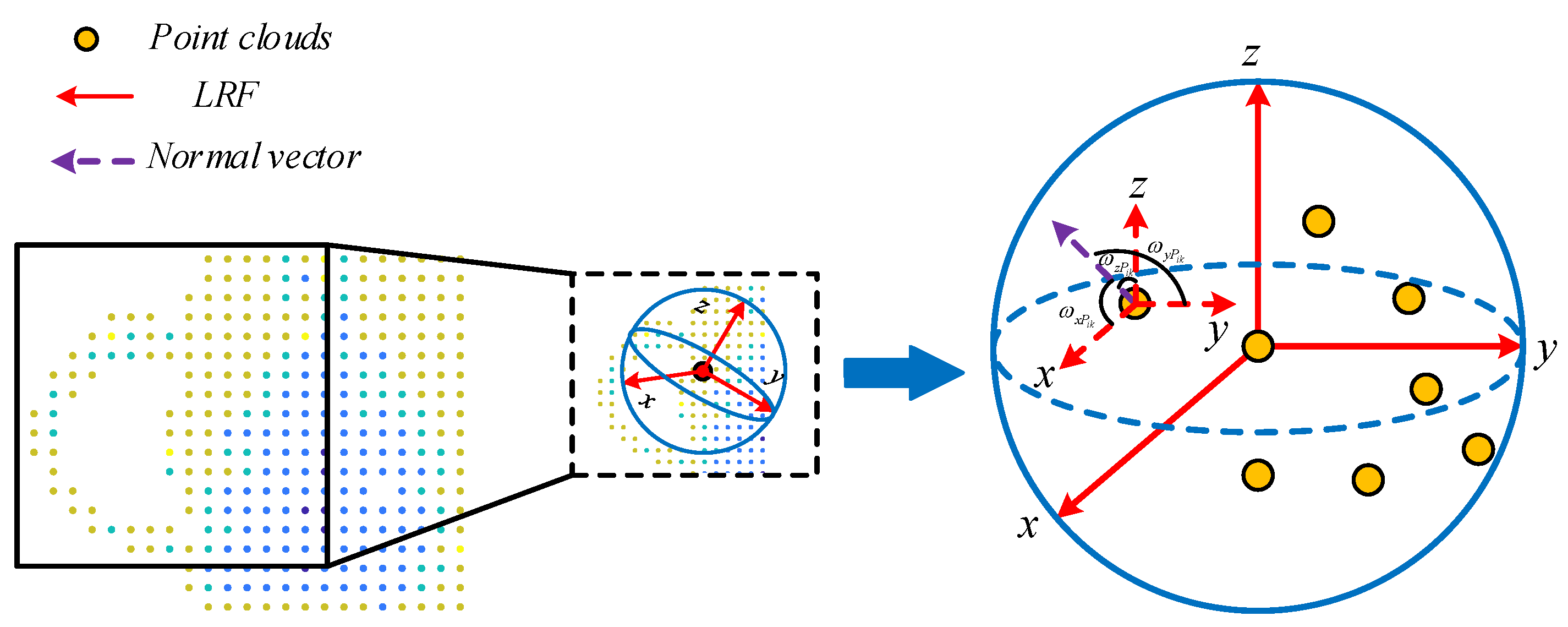
2.2.2. Feature of Normal Vectors Deviation Angle

In this section, we elaborate on the calculation method of the angular deviation feature between the normal vectors of each point in the point cloud and the LRF. We still take a point $P_i$ in $P$ as the example. The deviation angle mentioned here refers to the deviation angle between the normal vectors of each point in the feature point neighborhood of $P_i$ and the $x$, $y$, and $z$ axes of the LRF.

First, we use principal component analysis (PCA) [20] to calculate the normal vectors of each point in the point cloud. For a point $P_i(x_{P_i},y_{P_i},z_{P_i})$ in $P$, the barycenter of the feature point neighborhood is shown in Equation (6).

$$B_{P_i}\left(x_{B_{P_i}},y_{B_{P_i}},z_{B_{P_i}}\right)=\frac{{\displaystyle \sum _{j=1}^{n_{{}_{P_i}}}(x_{j{P}_i},y_{j{P}_i},z_{j{P}_i})}}{n_{{}_{P_i}}},$$

(6)

where $n_{{}_{P_i}}$ is the number of points in the feature point neighborhood of $P_i$. Then, we construct the covariance matrix for $P_{ik}$:

$$Cov\left(P_{ik}\right)={\displaystyle \sum _{j=1}^{n_{{}_{P_i}}}\left(P_{i{k}_j}-B_{P_i}\right)}{\left(P_{i{k}_j}-B_{P_i}\right)}^T,$$

(7)

$$Cov\left(P_{ik}\right)={\left[\begin{array}{l}{P}_{ik}^1-B_{P_i}\\ \cdot \cdot \cdot \\ P_{ik}^{n_{{}_{P_i}}}-B_{P_i}\end{array}\right]}^T•\left[\begin{array}{l}{P}_{ik}^1-B_{P_i}\\ \cdot \cdot \cdot \\ P_{ik}^{n_{{}_{P_i}}}-B_{P_i}\end{array}\right],$$

(8)

We calculate the eigenvalues and eigenvectors of $Cov\left(P_{ik}\right)$, where the eigenvectors are the normal vector $\overrightarrow{{\lambda }_{P_{ik}}}$ of $P_{ik}$. Then, we calculate the deviation angles between $\overrightarrow{{\lambda }_{P_{ik}}}$ and $x$-, $y$-, and $z$-axes of the LRF, as shown in Equations (9)–(14).

$$\cos ({\omega }_{x{P}_{ik}})=\cos <\overrightarrow{{\delta }_{P_i{}_x}},\overrightarrow{{\lambda }_{P_{ik}}}>=(\overrightarrow{{\delta }_{P_i{}_x}}•\overrightarrow{{\lambda }_{P_{ik}}})/(\left|\overrightarrow{{\delta }_{P_i{}_x}}\right|\left|\overrightarrow{{\lambda }_{P_{ik}}}\right|),$$

(9)

$$\cos ({\omega }_{y{P}_{ik}})=\cos <\overrightarrow{{\delta }_{P_i{}_y}},\overrightarrow{{\lambda }_{P_{ik}}}>=(\overrightarrow{{\delta }_{P_i{}_y}}•\overrightarrow{{\lambda }_{P_{ik}}})/(\left|\overrightarrow{{\delta }_{P_i{}_y}}\right|\left|\overrightarrow{{\lambda }_{P_{ik}}}\right|),$$

(10)

$$\cos ({\omega }_{z{P}_{ik}})=\cos <\overrightarrow{{\delta }_{P_i{}_z}},\overrightarrow{{\lambda }_{P_{ik}}}>=(\overrightarrow{{\delta }_{P_i{}_z}}•\overrightarrow{{\lambda }_{P_{ik}}})/(\left|\overrightarrow{{\delta }_{P_i{}_z}}\right|\left|\overrightarrow{{\lambda }_{P_{ik}}}\right|),$$

(11)

$${\omega }_{x{P}_{ik}}=\mathrm{arc}\cos (\overrightarrow{{\delta }_{P_i{}_x}},\overrightarrow{{\lambda }_{P_{ik}}})/(|\overrightarrow{{\delta }_{P_i{}_x}}\left|\right|\overrightarrow{{\lambda }_{P_{ik}}}|),$$

(12)

$${\omega }_{y{P}_{ik}}=\mathrm{arc}\cos (\overrightarrow{{\delta }_{P_i{}_y}},\overrightarrow{{\lambda }_{P_{ik}}})/(|\overrightarrow{{\delta }_{P_i{}_y}}\left|\right|\overrightarrow{{\lambda }_{P_{ik}}}|),$$

(13)

$${\omega }_{z{P}_{ik}}=\mathrm{arc}\cos (\overrightarrow{{\delta }_{P_i{}_z}},\overrightarrow{{\lambda }_{P_{ik}}})/(|\overrightarrow{{\delta }_{P_i{}_z}}\left|\right|\overrightarrow{{\lambda }_{P_{ik}}}|),$$

(14)

where $\cos ({\omega }_{x{P}_{ik}})$, $\cos ({\omega }_{y{P}_{ik}})$, and $\cos ({\omega }_{z{P}_{ik}})$ are the cosines of the deviation angle between $\overrightarrow{{\lambda }_{P_{ik}}}$ and the $x$-, $y$-, and $z$-axes of the LRF, respectively. ${\omega }_{x{P}_{ik}}$, ${\omega }_{y{P}_{ik}}$, and ${\omega }_{z{P}_{ik}}$ are the deviation angle between $\overrightarrow{{\lambda }_{P_{ik}}}$ and the $x$-, $y$-, and $z$-axes of the LRF, respectively. The deviation angle between the normal vector and the LRF is shown in Figure 4.

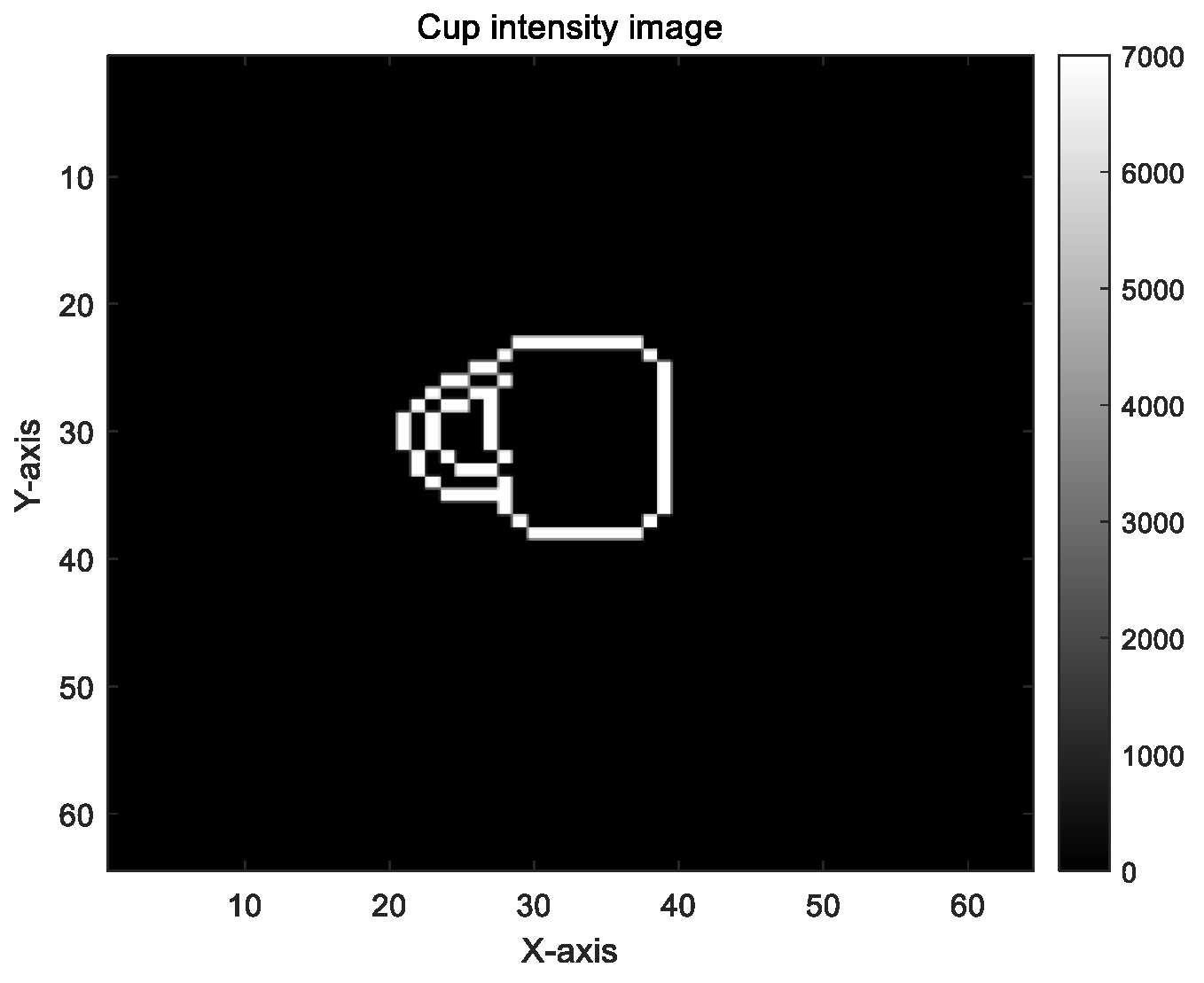
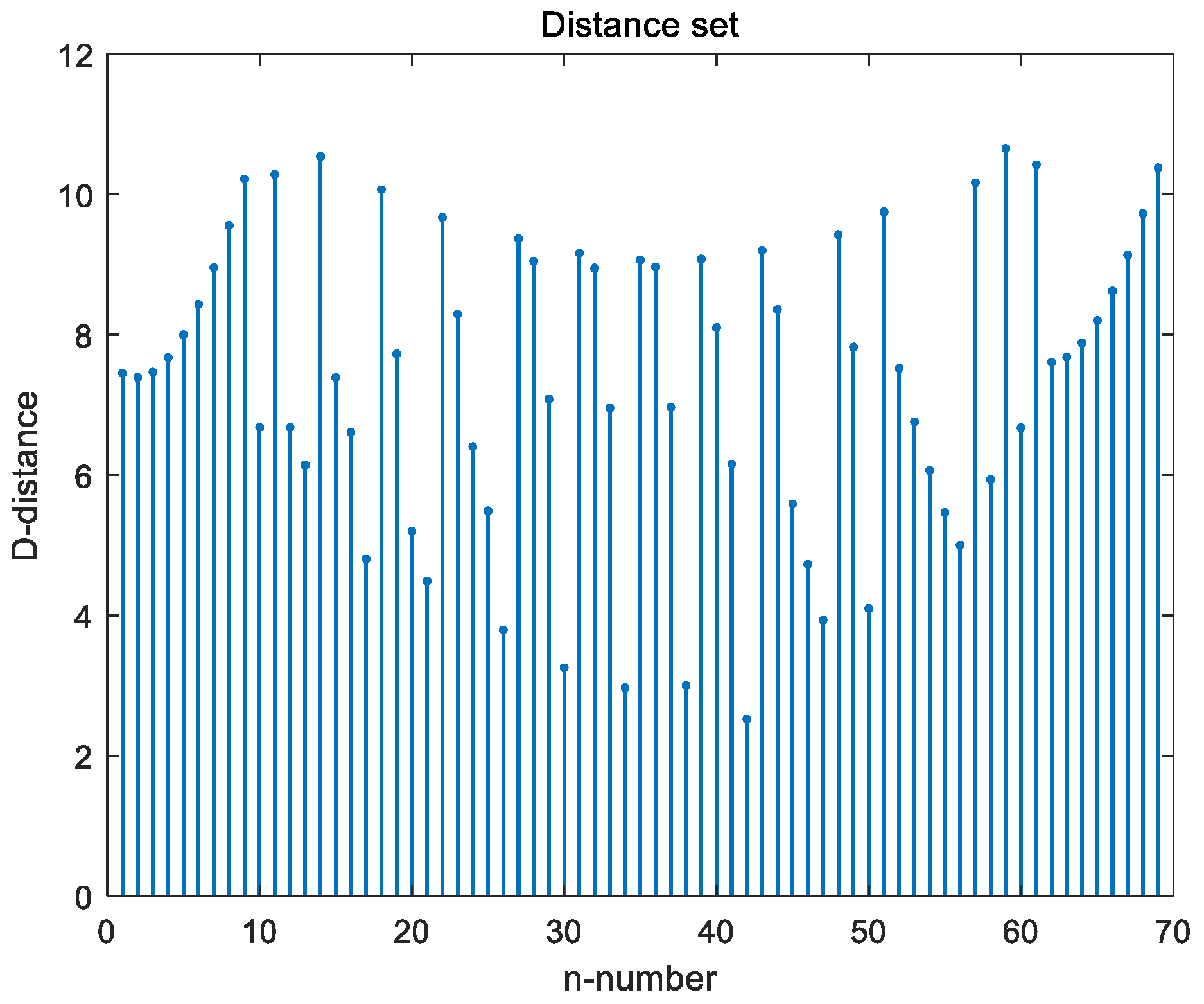
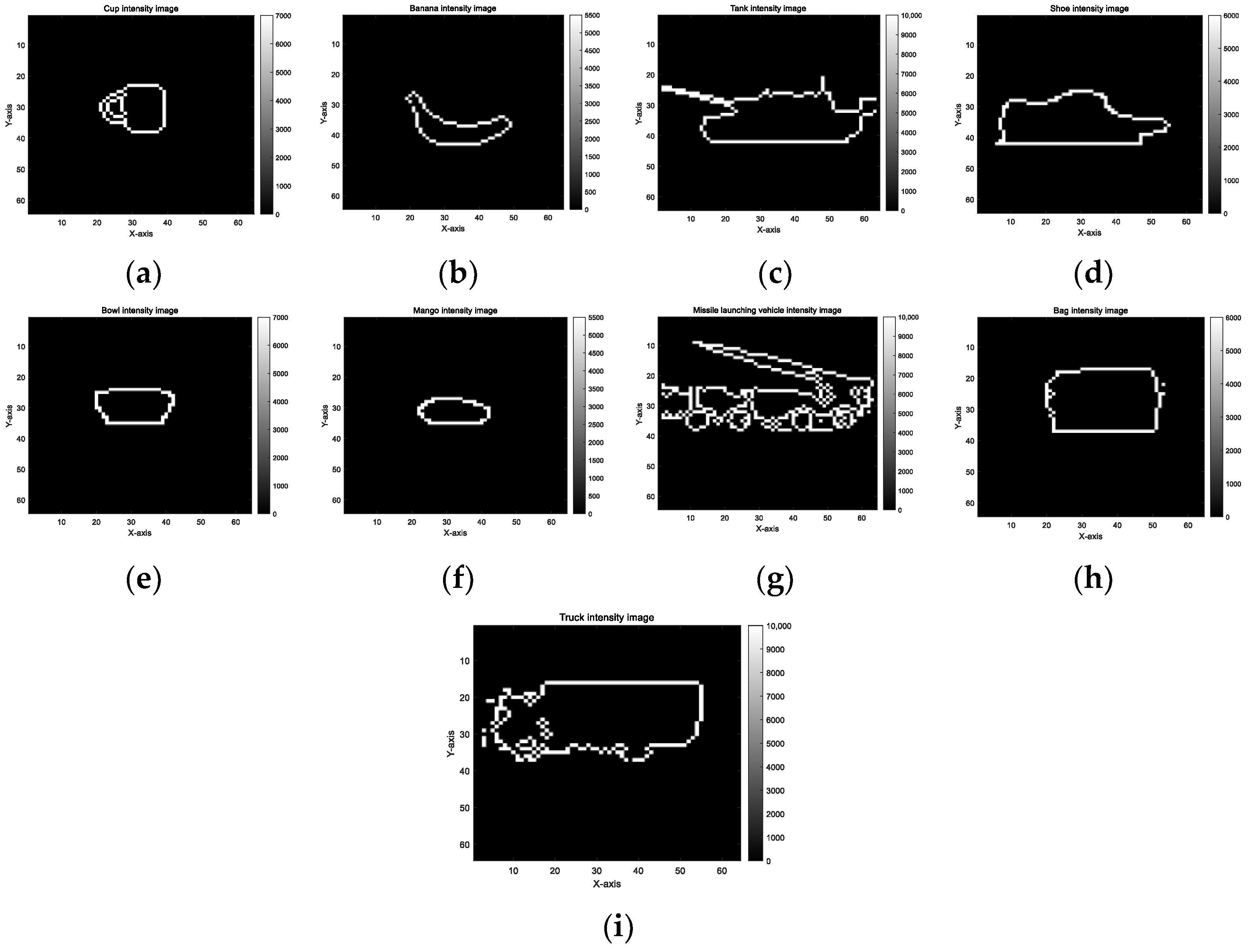
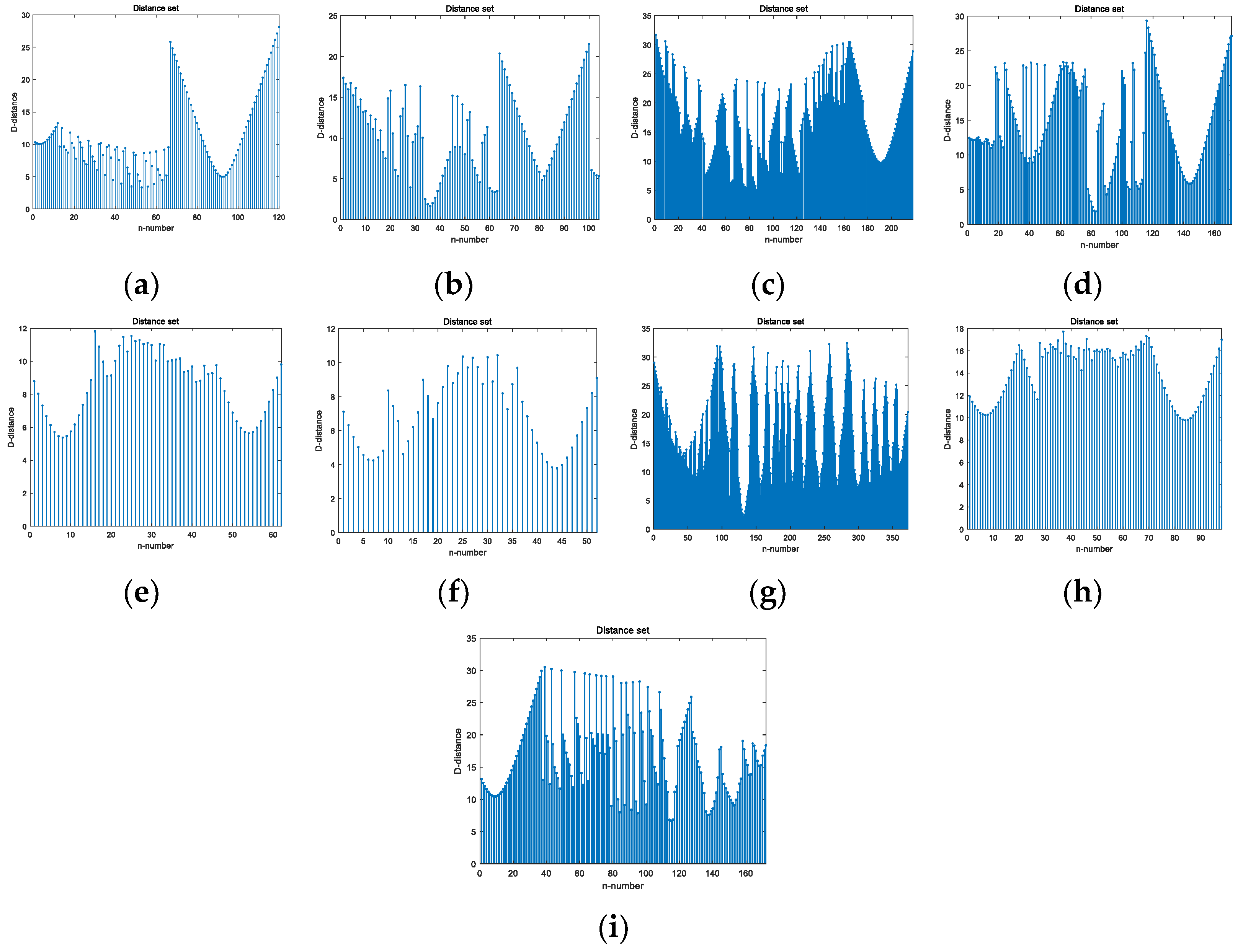
2.3. Contour Fourier Feature of the Intensity Image

The APD array LiDAR can obtain the point cloud and intensity information of the object, making full use of the intensity information to improve the accuracy of the object recognition method. Because the number of APD arrays is fixed, the pixels of the detected point cloud and the intensity image are equal, which omits the registration process of two different images. In this section, we derive the calculation method of the intensity feature in detail.

We extract the contour information of the object in the scene. We use the Improved Canny edge detection algorithm to extract the contour of the object [21], as shown in Figure 5.

In order to calculate the intensity feature of the object more accurately, we perform image segmentation on the intensity image of the object. The distance $d_{p_1{p}_2}$ between pixels $c_1=(x_1,y_1)$ and $c_2=(x_2,y_2)$ in the intensity image is represented by the following:

$$d_{p_1{p}_2}=\sqrt{{\left(x_1-x_2\right)}^2+{\left(y_1-y_2\right)}^2},$$

(15)

Randomly select an arbitrary pixel $C_m$ in the intensity image and calculate the distance set $G_{C_m}$ between each pixel in the intensity image and $C_m$. Store the elements in $G_{C_m}$ that are less than the threshold of 0.5 in an empty set $J_{C_m}$. If no new elements are added to $J_{C_m}$, the segmentation is complete; if new elements continue to be added to $J_{C_m}$, select a point in $J_{C_m}$ other than point $C_m$ as the new $C_m$ point and perform the above operation until no new elements are added to $J_{C_m}$. Based on the above steps, we can segment the object intensity image, extract the object from the background, and make the subsequent feature calculations more accurate. Intensity image after image segmentation is shown in Figure 6.

The contour of the object is composed of N pixels, and each point p can be regarded as a vector, where its complex number expression is obtained as

$$l_q=\begin{array}{cc}{x}_q+i{y}_q,& q=1,2,\cdot \cdot \cdot ,n\end{array},$$

(16)

The coordinate of the barycenter of the contour $b\left(x_b,y_b\right)$ is obtained as

$$b\left(x_b,y_b\right)=\left(\frac{1}{n}{\displaystyle \sum _{i=1}^n{x}_i,\frac{1}{n}{\displaystyle \sum _{i=1}^n{y}_i}}\right),$$

(17)

Select any pixel in the contour as the starting point and calculate the distance between each pixel of the contour and the barycenter in turn, as shown in Equation (18).

$$d(i)={\left[{\left(x_i-x_b\right)}^2+{\left(y_i-y_b\right)}^2\right]}^{1/2},$$

(18)

Combine the calculated $n$ distances into a distance set $D=\left\{d_1,d_2,\cdot \cdot \cdot ,d_n\right\}$, as shown in Figure 7. The DFT of $D$ is performed to obtain the Fourier feature of the contour of the object, as shown in Equation (19).

$$D(k)=DFT(D)=\begin{array}{cc}\frac{1}{n}{\displaystyle \sum _{i=1}^{n}d(i)\exp }\left(\frac{-j2\pi ki}{n}\right),& k=1,2,\cdot \cdot \cdot ,n\end{array},$$

(19)

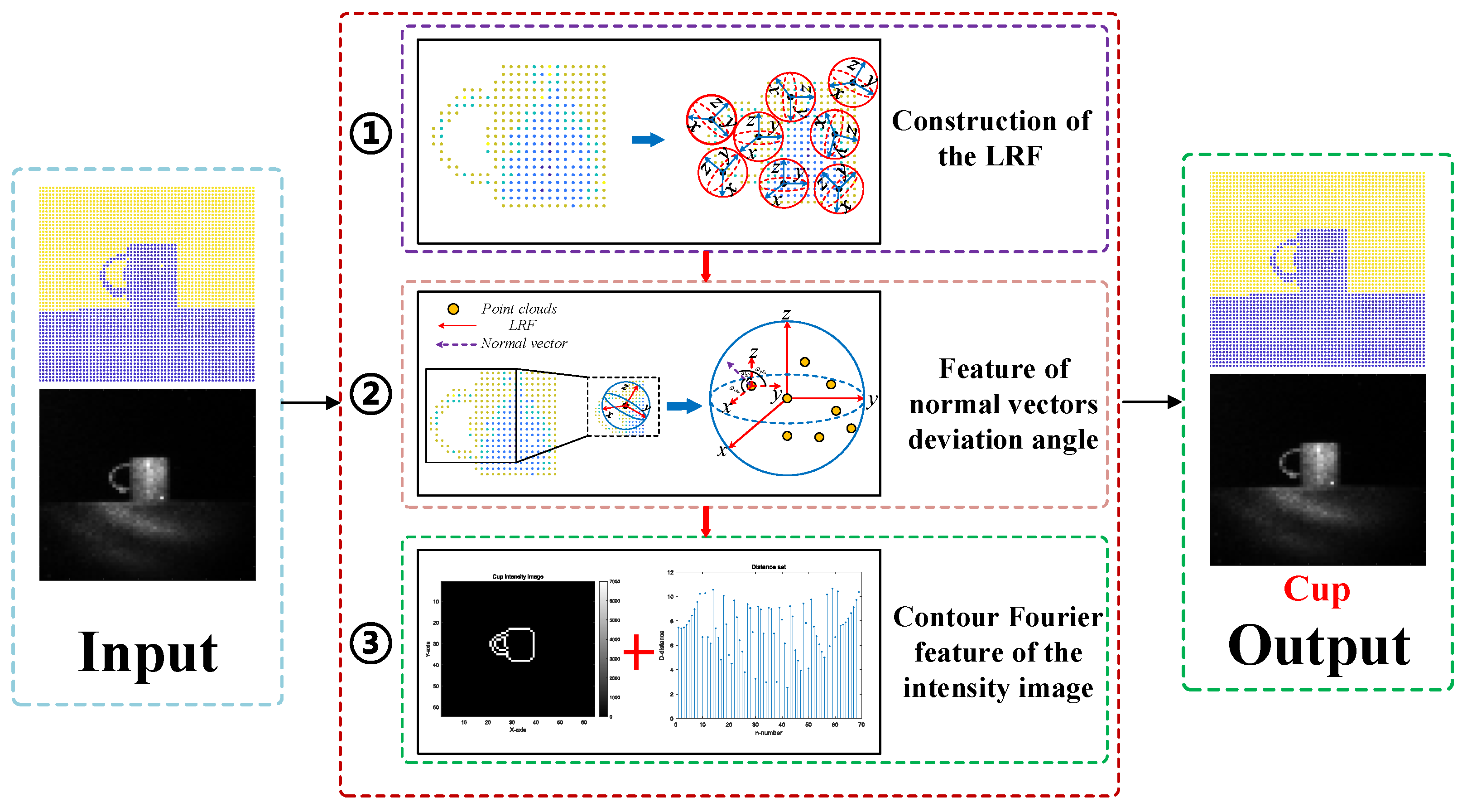
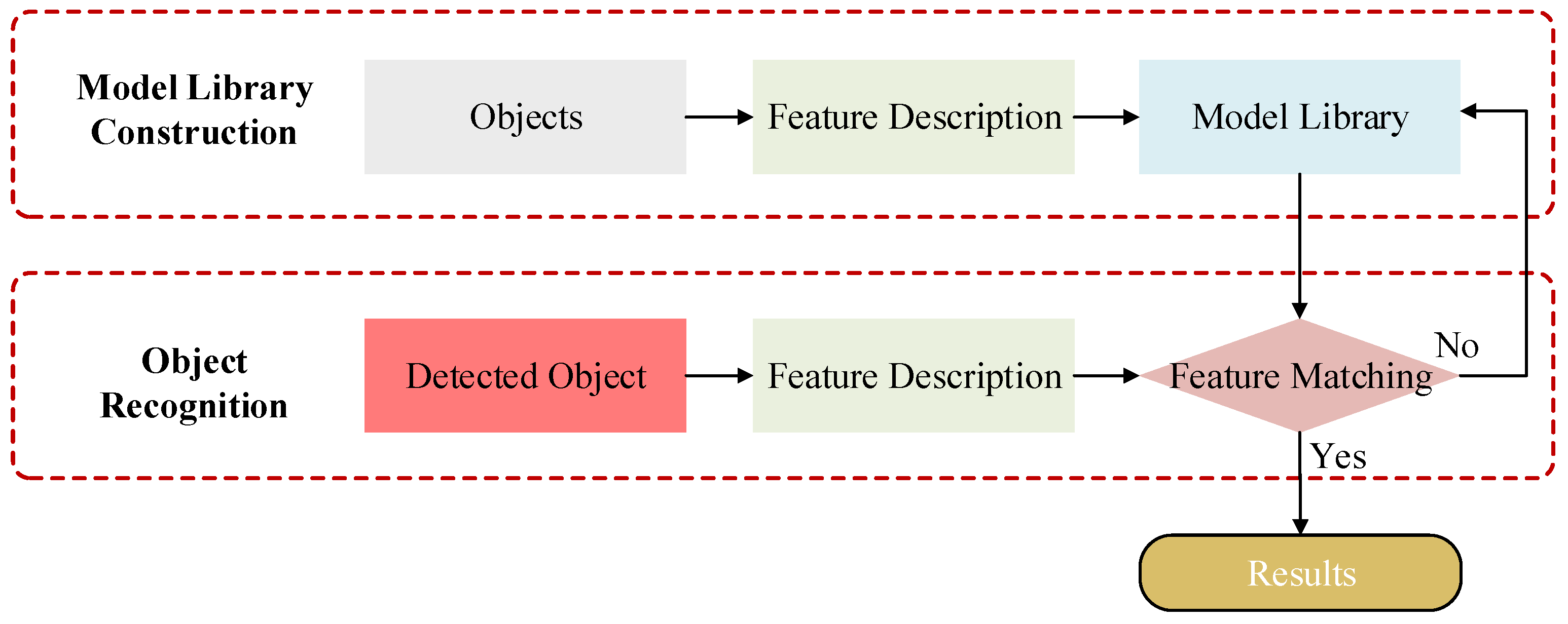
2.4. Object Recognition Process

In this section, we illustrate how to use the proposed object recognition method to recognize objects. The whole process of object recognition is divided into two stages: model library construction and object recognition. The purpose of the model library construction stage is to obtain prior knowledge about the objects. To this end, we use a 64 × 64 array APD LiDAR to detect various types of objects and apply the proposed object recognition method for feature description. The calculated object feature information is stored, thus creating a model library. In the stage of object recognition, we use APD LiDAR to detect the object and still employ the proposed object recognition method for feature description of the obtained point cloud and intensity image. We then match the calculated results with the model library, and if the features match successfully with a certain type of object in the library, we consider it to be that type. The flow chart of the object recognition process is shown in Figure 8.

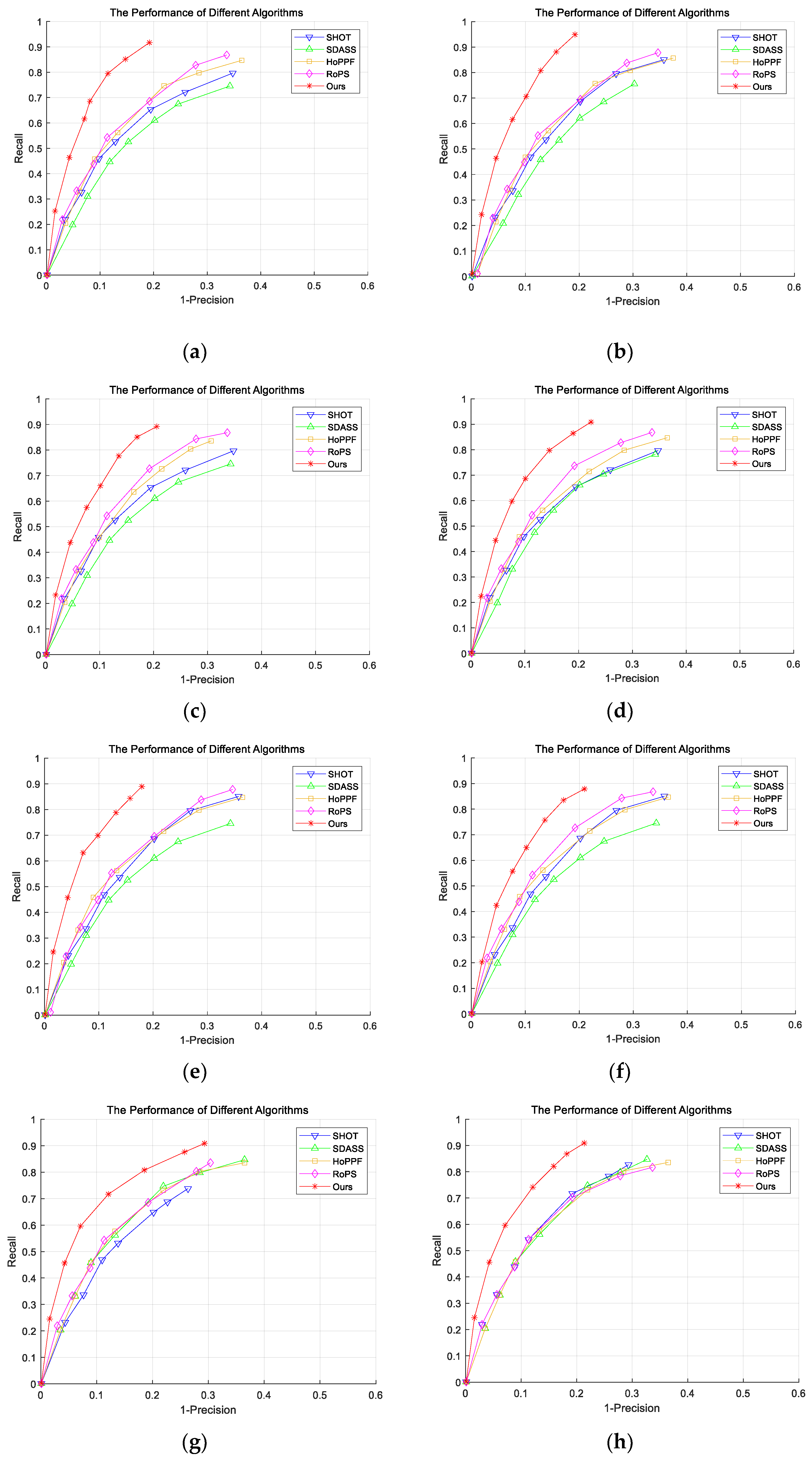
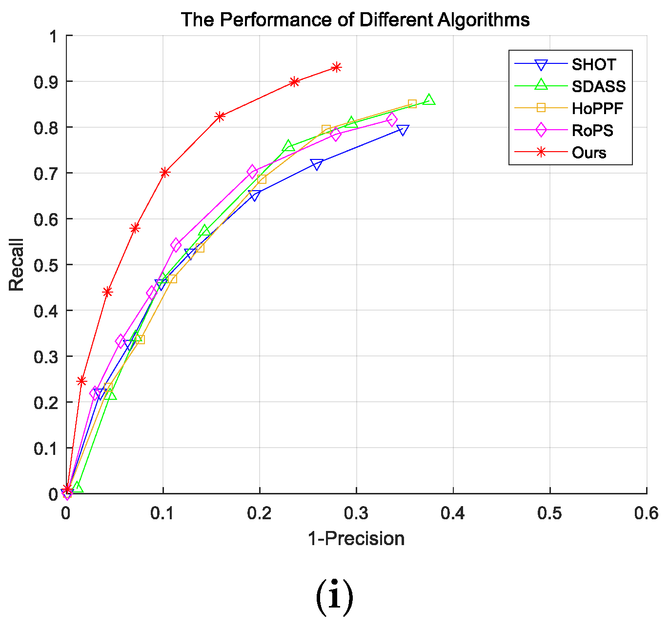
3. Experimental Results

In this section, the proposed object recognition method is tested with the APD LiDAR detection data. Additionally, we compare the performance of the proposed method with that of the SHOT [6], SDASS [7], HoPPF [8], and RoPS [9] algorithms to demonstrate the advantages in terms of descriptiveness, robustness, and computational efficiency. All experiments were implemented in MATLAB and conducted on a computer with an Intel Core 3.6–GHz processor and 16 GB of RAM. To quantitatively evaluate the performance of the proposed object recognition method, we used the RPC criterion [6,10]. The calculations for the RPC criterion are as follows.

Select 1000 key points randomly from the object and locate their corresponding points through ground-truth transformation [9,10]. Calculate the features of the object to be identified and match them with the model library and then find the features with the minimum matching error. When the matching error is less than 0.5 r, the matching is considered correct. We use $\mathrm{recall}$ and $1-\mathrm{precision}$ as evaluation indicators. $\mathrm{recall}$ is calculated according to the number of correct feature point matches and the number of corresponding key point pairs, and $1-\mathrm{precision}$ is calculated according to the number of false feature point matches and the total number of feature point matches. They are expressed as:

$$\mathrm{recall}=\frac{\mathrm{number} \mathrm{of} \mathrm{correct} \mathrm{matches}}{\mathrm{total} \mathrm{number} \mathrm{of} \mathrm{corresponding} \mathrm{features}},$$

(20)

$$1-\mathrm{precision}=\frac{\mathrm{number} \mathrm{of} \mathrm{false} \mathrm{matches}}{\mathrm{total} \mathrm{number} \mathrm{of} \mathrm{matches} },$$

(21)

If an object recognition method has both high a $\mathrm{recall}$ and $1-\mathrm{precision}$, its RPC curve should be located in the upper left of the plot [8]. The parameter settings for the proposed method and compared methods are shown in

Table 1. The parameter settings for the proposed method and compared methods.

	Support Radius/ Mesh Resolution (mr)	Dimensionality	Length
Ours	15	8 × 4 × 4 × 8	350
SHOT	15	8 × 2 × 2 × 10	340
SDASS	15	15 × 5 × 5	335
HoPPF	15	8 × 3 × 5 × 5	600
RoPS	15	3 × 3 × 3 × 5	135

.

We used APD array LiDAR to conduct detection imaging on images of a Cup, Banana, Tank model, shoe, bowl, mango, missile launching vehicle model, and bag and truck model and used them to test the descriptive and computational efficiency of the proposed method. The results are shown in Figure 9, Figure 10, Figure 11, Figure 12, Figure 13 and Figure 14 and

Table 2. Comparison of the computing times.

Times/s	SHOT	SDASS	HoPPF	RoPS	Ours
Cup	0.092	0.067	0.052	0.061	0.049
Banana	0.081	0.056	0.044	0.052	0.037
Tank	0.188	0.109	0.088	0.096	0.088
Shoe	0.142	0.087	0.069	0.085	0.080
Bowl	0.087	0.060	0.048	0.054	0.045
Mango	0.079	0.052	0.041	0.050	0.038
Missile-launching vehicle	0.258	0.149	0.138	0.143	0.121
Bag	0.124	0.095	0.083	0.088	0.072
Truck	0.182	0.123	0.106	0.109	0.099
Average computing times	0.1370	0.0887	0.0743	0.0820	0.0699

. Each point of the RPC curve in Figure 15 represents a different matching threshold. We can see that the proposed object recognition method has the best performance, followed by RoPS. This obvious advantage is because the proposed algorithm utilizes both the spatial features and intensity features of the point cloud of the object. In terms of being computationally efficient, the proposed method still has excellent performance, as shown in Table 2. The reason why the computing time of the proposed method does not have a significant advantage is that we have a variety of feature computation steps, which increases the certain time cost. However, because each step of the proposed method is very simple and effective, the computational efficiency of the proposed method is still very high.

4. Conclusions

In this paper, we propose a LiDAR point cloud object recognition method using intensity image compensation. The proposed method does not require cross-spectral image registration, and the added intensity information improves the description of the algorithm. We tested the performance of the proposed method with the APD array LiDAR data. The experimental results show that the RPC curve of the proposed method is better than that of the comparison methods, and the average computing time of the proposed method is 0.0699 s, which is better than the comparison methods. In summary, it can be seen that the proposed method is highly descriptive and computationally efficient.

In our future work, we will focus on the following two directions: (1) we will consider adding the RGB information of the target into the feature description to improve the performance of the proposed method. (2) We plan to combine the proposed object recognition method with deep learning, adopt the idea of deep learning to train the point cloud and intensity features of objects, and improve the performance of the object recognition method with a large amount of prior knowledge of objects.

References

1. Tan, H.; Peng, J.Y.; Xiong, Z.W.; Liu, D.; Huang, X.; Li, Z.P.; Hong, Y.; Xu, F.H. Deep Learning Based Single–Photon 3D Imaging with Multiple Returns. In Proceedings of the International Conference on 3D Vision (3DV), Fukuoka, Japan, 25–28 November 2020. [Google Scholar] [CrossRef]
2. Nguyen, C.V.; Izadi, S.; Lovell, D. Modeling kinect sensor noise for improved 3D reconstruction and tracking. In Proceedings of the IEEE Second International Conference on 3D Imaging, Modeling, Processing, Visualization & Transmission, Zurich, Switzerland, 13–15 October 2012. [Google Scholar] [CrossRef]
3. Broggi, A.; Buzzoni, M.; Debattisti, S.; Grisleri, P.; Laghi, M.C.; Medici, P.; Versari, P. Extensive Tests of Autonomous Driving Technologies. IEEE Trans. Intell. Transp. Syst. 2013, 14, 1403–1415. [Google Scholar] [CrossRef]
4. Seo, Y.W.; Lee, J.; Zhang, W.; Werrergreen, D. Recognition of highway work zones for reliable autonomous driving. IEEE Trans. Intell. Transp. Syst. 2015, 16, 708–718. [Google Scholar] [CrossRef]
5. Chen, X.Z.; Ma, H.M.; Wan, J.; Li, B.; Xia, T. Multi–view 3D object detection network for autonomous driving. In Proceedings of the IEEE Conference on Computer Vision and Pattern Recognition (CVPR), Honolulu, HI, USA, 21–26 July 2017. [Google Scholar] [CrossRef]
6. Tombari, F.; Salti, S.; Stefano, L.D. Unique signatures of histograms for local surface description. In Proceedings of the European Conference on Computer Vision (ECCV), Heraklion, Crete, Greece, 5–11 September 2010. [Google Scholar] [CrossRef]
7. Zhao, B.; Le, X.Y.; Xi, J.T. A novel SDASS descriptor for fully encoding the information of a 3D local surface. Inf. Sci. 2019, 483, 363–382. [Google Scholar] [CrossRef]
8. Zhao, H.; Tang, M.J.; Ding, H. HoPPF: A novel local surface descriptor for 3D object recognition. Pattern Recognit. 2020, 103, 107272. [Google Scholar] [CrossRef]
9. Guo, Y.L.; Sohel, F.; Bennamoun, M.; Lu, M.; Wan, J.W. Rotational projection statistics for 3D local surface description and object recognition. Int. J. Comput. Vis. 2013, 105, 63–86. [Google Scholar] [CrossRef]
10. Guo, Y.L.; Bennamoun, M.; Sohel, F.; Lu, M.; Wan, J.; Kwok, N.M. A comprehensive performance evaluation of 3D local feature descriptors. Int. J. Comput. Vis. 2016, 116, 66–89. [Google Scholar] [CrossRef]
11. Ge, Z.X.; Shen, X.L.; Gao, Q.Q.; Sun, H.Y.; Tang, X.A.; Cai, Q.Y. A Fast Point Cloud Recognition Algorithm Based on Keypoint Pair Feature. Sensors 2022, 22, 6289. [Google Scholar] [CrossRef] [PubMed]
12. Charles, R.Q.; Su, H.; Kaichun, M.; Guibas, L.J. PointNet: Deep Learning on Point Sets for 3D Classification and Segmentation. In Proceedings of the IEEE Conference on Computer Vision and Pattern Recognition (CVPR), Honolulu, HI, USA, 21–26 July 2017. [Google Scholar] [CrossRef]
13. Qi, C.R.; Li, Y.; Hao, S.; Guibas, L.J. Pointnet++: Deep hierarchical feature learning on point sets in a metric space. In Proceedings of the 31st International Conference on Neural Information Processing Systems (NIPS), Long Beach, CA, USA, 4–9 December 2017. [Google Scholar] [CrossRef]
14. Maturana, D.; Scherer, S. Voxnet: A 3d convolutional neural network for real–time object recognition. In Proceedings of the IEEE/RSJ International Conference on Intelligent Robots and Systems (IROS), Hamburg, Germany, 28 September–2 October 2015. [Google Scholar] [CrossRef]
15. Liu, D.R.; Chen, C.C.; Xu, C.Q.; Cai, Q.; Chu, L.; Wen, F.; Qiu, R. A Robust and Reliable Point Cloud Recognition Network Under Rigid Transformation. IEEE Trans. Instrum. Meas. 2022, 71, 1–13. [Google Scholar] [CrossRef]
16. Jin, S.; Wu, Z.; Zhao, C.; Zhang, J.; Peng, G.; Wang, D. SectionKey: 3–D Semantic Point Cloud Descriptor for Place Recognition. In Proceedings of the IEEE/RSJ International Conference on Intelligent Robots and Systems (IROS), Kyoto, Japan, 23–27 October 2022. [Google Scholar] [CrossRef]
17. Zhao, H.S.; Jiang, L.; Jia, J.Y.; Torr, P.; Koltun, V. Point Transformer. In Proceedings of the IEEE/CVF International Conference on Computer Vision (ICCV), Montreal, QC, Canada, 10–17 October 2021. [Google Scholar] [CrossRef]
18. Qian, R.; Lai, X.; Li, X. BADet: Boundary–Aware 3D Object Detection from Point Clouds. Pattern Recognit. 2022, 125, 108524. [Google Scholar] [CrossRef]
19. Yang, J.Q.; Zhang, Q.; Xiao, Y.; Cao, Z.G. TOLDI: An effective and robust approach for 3d local shape description. Pattern Recognit. 2017, 65, 175–187. [Google Scholar] [CrossRef]
20. Mitra, N.J.; Nguyen, A.; Guibas, L. Estimating surface normals in noisy point cloud data. Int. J. Comput. Geom. Appl. 2004, 14, 261–276. [Google Scholar] [CrossRef]
21. Rong, W.; Li, Z.; Zhang, W.; Sun, L. An improved Canny edge detection algorithm. In Proceedings of the IEEE International Conference on Mechatronics and Automation (ICMA), Tianjin, China, 3–6 August 2014. [Google Scholar] [CrossRef]
Figure 1. Schematic diagram of detection using APD array LiDAR.
Electronics 12 02087 g001
Figure 2. The flow chart of the proposed method.
Electronics 12 02087 g002
Figure 3. Construct the LRF for each point in the input point cloud P .
Electronics 12 02087 g003
Figure 4. The deviation angle between the normal vector and the LRF.
Electronics 12 02087 g004
Figure 5. Contour extraction of Cup. (a) Photograph of cup; (b) the intensity image of the Cup; (c) contour information of the Cup.
Electronics 12 02087 g005
Figure 6. The intensity image after image segmentation.
Electronics 12 02087 g006
Figure 7. The set of distances between the contour and the barycenter.
Electronics 12 02087 g007
Figure 8. The flow chart of the object recognition process.
Electronics 12 02087 g008
Figure 9. The photographs of the detected objects. (ai) are the cup, banana, tank, shoe, bowl, mango, missile-launching vehicle, bag, and truck models, respectively.
Electronics 12 02087 g009
Figure 10. The point cloud of the detected objects. (ai) are the cup, banana, tank, shoe, bowl, mango, missile-launching vehicle, bag, and truck models, respectively.
Electronics 12 02087 g010
Figure 11. The intensity images of the detected objects. (ai) are the cup, banana, tank, shoe, bowl, mango, missile-launching vehicle, bag, and truck models, respectively.
Electronics 12 02087 g011
Figure 12. The edge detection results using Improved Canny algorithm. (ai) are the cup, banana, tank, shoe, bowl, mango, missile-launching vehicle, bag, and truck models, respectively.
Electronics 12 02087 g012
Figure 13. Intensity image after image segmentation. (ai) are the cup, banana, tank, shoe, bowl, mango, missile-launching vehicle, bag, and truck models, respectively.
Electronics 12 02087 g013
Figure 14. The set of distances of the detected objects. (ai) are the cup, banana, tank, shoe, bowl, mango, missile-launching vehicle, bag, and truck models, respectively.
Electronics 12 02087 g014
Figure 15. Descriptive tests of the proposed method with the (a) cup, (b) banana, (c) tank, (d) shoe, (e) bowl, (f) mango, (g) missile-launching vehicle, (h) bag, and (i) truck models.
Electronics 12 02087 g015aElectronics 12 02087 g015b