An AI-Based Power Reserve Control Strategy for Photovoltaic Power Generation Systems Participating in Frequency Regulation of Microgrids

Abstract

In this paper, a novel AI-based power reserve control strategy is proposed for photovoltaic (PV) power generation systems participating in the frequency regulation (FR) of microgrids. The proposed strategy uses a frequency response module to determine the target power reserve ratio of the PV system based on microgrid frequency deviation, as well as a power reserve control module to obtain the target duty cycle, which is input to the BOOST converter. The use of artificial neural networks (ANN) in the power reserve control module enables the PV system to work at a specified power reserve ratio, producing appropriate power and mitigating frequency fluctuations in the microgrid. Additionally, a deep reinforcement learning (DRL) algorithm is employed as the decision maker for variable step-size control and initial power reserve ratio determination. Simulations were performed to validate the effectiveness of the proposed method, demonstrating a significant reduction in average frequency deviation by 72.36% when subjected to random variations in irradiance intensity and load conditions. Overall, the proposed AI-based power reserve control strategy has good potential for practical applications in real-world microgrids, promoting the absorption of new energy led by PV and reducing the phenomenon of light abandonment.

1. Introduction

In recent years, the economic and environmental benefits of photovoltaic (PV) technology have made it increasingly popular for power generation in microgrids [1,2]. However, the integration of a large number of PV sources has also introduced a new threat to the operational safety and stability of microgrids. These challenges arise primarily from three aspects: (i) the volatile and random output of PV sources negatively impacts the power balance of microgrids [3,4], and unbalanced active power in microgrids causes deviations from the standard operating frequency; (ii) as PV power generation systems (PV systems) do not respond to frequency deviations in the microgrid, the frequency regulation (FR) capacity, mainly provided by synchronous generators in microgrids, is occupied, and the frequency regulation ability of microgrids is thereby reduced [5]; and (iii) the use of inverters instead of synchronous generators diminishes the overall inertia of microgrids [6], limiting their inherent ability to overcome frequency disturbances. The combination of these factors significantly reduces the frequency stability of microgrids with high PV penetration rates [7], which results in poor power quality for users and poses challenges to the reliable and consistent functioning of power system equipment. Therefore, there is an increasing operational demand for PV systems to participate in FR, especially in small-sized and isolated microgrids with high PV penetration rates [8,9].

To participate in FR, PV systems need to control a portion of the active power to mimic frequency regulation capacity [10]. Three main approaches are currently available: (i) installation of energy storage devices [11,12]; (ii) application of a synchronverter, also known as a virtual synchronous generator (VSG) [13,14]; and (iii) utilizing power reserve control, which makes the PV operating point deviate from the maximum power point (MPP) [15,16,17,18,19,20,21,22]. However, extensive performance analyses of a variety of energy storage devices in microgrid environments have concluded that energy storage systems are not economically feasible due to their shorter lifespan and higher investment cost compared with PV system components [23]. Furthermore, the possibility of deriving frequency regulation from PV systems without energy storage has been explored [24]. Therefore, it is desirable for PV systems to provide up- and downregulation of active power in high-penetration applications without relying on energy storage. Meanwhile, VSG-based approaches are more appropriate for creating a brand-new PV inverter system with modifications to both hardware and software [14]. Despite their commendable performances, these approaches are not economical for grid-following PV plants that are already in operation on a large scale. As a result, power reserve control is a more practical approach for grid-following PV plants on a large scale. Considering the above-mentioned aspects, this study centers on the utilization of the power reserve control approach as the primary methodology.

The critical task of power reserve control is to accurately determine a suitable operating point for the PV system, which requires obtaining sufficient information on the characteristic curve of the PV array under a given condition. The ways to realize this can be divided into two categories: direct measurement and real-time estimation. As an example of the former category, ref. [15] used a master PV system operating in maximum power point track (MPPT) mode to measure the maximum available power (MAP), which was then used by slave PV systems to control the operating point. Nevertheless, this approach is limited to large-scale PV plants with uniform component conditions and necessitates the use of a communication system. Other methods belonging to the former category, such as those described in [16,17], made PV systems operate alternatively in MPPT mode and power reserve control mode, with MAP measured and utilized in the same way. However, these two methods result in excess energy on DC-link capacitors, causing the DC-bus voltage to exceed the limit. Additionally, the methods in the first category often determine the target operating point according to the relationship between the target PV power and MAP, which increases the risk of sacrificing operational stability as the P-V curve is not monotonic, and operating on the left side of a P-V curve is an unstable state for a PV system [18].

The latter category, which is more common in the literature, involves determining the operating point of the PV systems by estimating important properties of the P-V characteristic curve. In [19], a voltage offset was added directly to the voltage of MPP, denoted as $V_{\mathrm{m}\mathrm{p}}$, under standard test conditions (STC) to achieve a quantitative deviation from the MPP. However, this method lacks consideration of changes in external conditions, resulting in decreased accuracy when tracking the target operating point. In [20], the mathematical relation between the current of the PV array and irradiance intensity, cell temperature, and voltage of the PV array was approximated by off-line curve fitting. In [21], a simplified PV array model was utilized to estimate the P-V characteristic curve under a given external condition by substituting the value of irradiance intensity and cell temperature into the model. In [5], the parameters of a quadratic curve were estimated by employing the least squares method on a substantial number of measurement samples collected around a set of operating points, resulting in enhanced robustness of the approach in the presence of noise. However, the nonlinearity and susceptibility to external environmental influences of the PV characteristic curve limit the accuracy of the methods proposed by these three studies when tracking target operating points, which compromises the frequency support ability of PV systems. Additionally, more precise methods are being researched and developed. One such method proposed in [22] involved iteratively solving the single-diode mathematical model of the PV array using the Newton–Raphson method to obtain information near the current operating point, allowing for determination of the necessary adjustment direction of the operating point. However, this iterative solution is computationally intensive and time-consuming, rendering it difficult to provide timely frequency support during severe fluctuations in the microgrid. Another method proposed in [10] estimated the target voltage offset from $V_{\mathrm{m}\mathrm{p}}$ through iterative calculation, while a variable-step strategy gradually moved the PV operating point to the target. However, the convergence speed of this approach needs improvement, and some key parameters were determined through manual experience, such as the initial power reserve ratio, which hindered the maximization of the balance between the frequency support ability of PV systems and the utilization rate of solar energy. In summary, the methods belonging to the second category overcome the harsh application conditions of the first category and avoid the risk of operational instability, but they also face new challenges in balancing tracking accuracy and computational speed.

To address the limitations of previous methods, a novel approach that leverages artificial intelligence (AI) has been proposed for power reserve control in PV systems participating in the FR of microgrids. This innovative approach overcomes the drawbacks of poor timeliness associated with the time-consuming solution of accurate mathematical equations and insufficient accuracy brought about by rough methods. The strategy begins with collecting the frequency deviation of the microgrid and utilizing a frequency response module to determine the target power reserve ratio of the PV system based on the measured frequency deviation. The decision-making process for determining the initial power reserve ratio is entrusted to a deep reinforcement learning (DRL) algorithm. Subsequently, a power reserve control module is employed to obtain the target duty cycle, where the DRL-based strategy facilitates intelligent variable step size, and the target duty cycle is then fed into the BOOST converter. With this control mechanism, the PV system is able to operate at the specified power reserve ratio, ensuring the generation of appropriate power and mitigating frequency fluctuations in the microgrid.

The major contributions and innovations of this paper are stated as two aspects:

(i)

A new AI-based power reserve control strategy is proposed for PV systems participating in the FR of microgrids, which effectively reduces the frequency deviation of microgrids with high PV permeability.

(ii)

A novel variable step-size strategy for BOOST converter duty cycle based on DRL is proposed, which allows PV systems to quickly converge to specified operating points even in the face of fluctuations in the external environment and load.

The remainder of this paper is structured as follows. Section 2 puts forward the control strategy for a PV power generation system participating microgrid FR. Section 3 proposes the DRL-based strategies for duty cycle variable step-size and optimal initial power reserve ratio selection. Section 4 presents the simulations and analysis of the results, and Section 5 concludes the paper with the key findings.

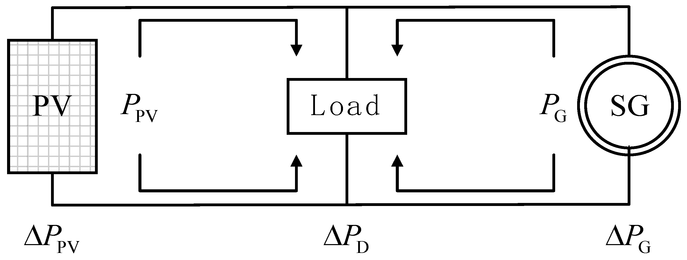
2. Frequency Regulation Strategy for PV Systems Based on Power Reserve Control

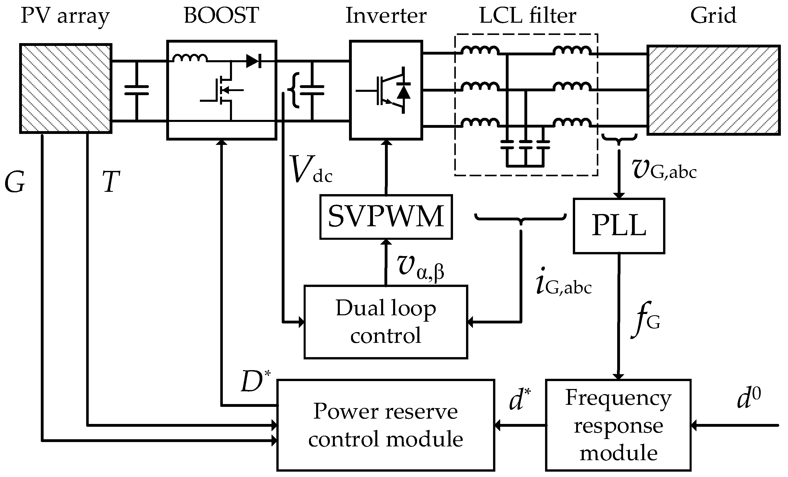
2.1. Basic Control Strategies for PV Power Reserve

As shown in Figure 1, a microgrid containing PV units can be simplified to a simple system consisting of only a PV system, a synchronous generator, and a load. It is worth mentioning that to accurately simulate frequency deviation caused by power imbalance in the microgrid, the idealized power grid initially connected to the PV system should be replaced with an equivalent load and a synchronous generator (SG) with limited capacity. The power transmitted by the PV system and the SG to the load is $P_{\mathrm{P}\mathrm{V}}$ and $P_{\mathrm{G}}$ respectively, and the power on the load is $P_{\mathrm{D}}$. Ignoring the network loss, the following relationship can be obtained:

$${P_{\mathrm{G}}+P}_{\mathrm{P}\mathrm{V}}=P_{\mathrm{D}}$$

(1)

when the power of PV or load fluctuates, (1) can be rewritten as

$$∆{P_{\mathrm{G}}+∆P}_{\mathrm{P}\mathrm{V}}={∆P}_{\mathrm{D}}$$

(2)

SGs will spontaneously participate in FR, and the output power will respond to changes in frequency [25]. The power–frequency static characteristic curve is shown in Figure 2, where $f_{\mathrm{N}}$ and $P_{\mathrm{G}\mathrm{N}}$ refer to the standard frequency of the grid and the rated power of the SG, respectively. The relationship between the frequency deviation $∆f$ and the output power change $∆P_{\mathrm{G}}$ is shown in Equation (3).

$$∆P_{\mathrm{G}}=-k_{\mathrm{G}}∆f$$

(3)

where $k_{\mathrm{G}}$ is the droop coefficient of the SG set by the power plant.

According to (2) and (3), when the power of PV and load fluctuate, the frequency deviation of the system is

$$∆f=\frac{∆P_{\mathrm{D}}-∆P_{\mathrm{P}\mathrm{V}}}{-k_{\mathrm{G}}}$$

(4)

It can be seen from (4) that the variability of both PV power and load can accumulate and affect the microgrid frequency, resulting in a higher maximum frequency deviation than that observed in the microgrid without PV power generation. Nevertheless, if PV systems can mitigate their inherent volatility and respond to the grid’s frequency deviation alongside conventional power generation units, the impact of PV integration on microgrid frequency can transition from negative to positive. In light of (3), the power–frequency static characteristics of a PV system can be defined as

$$∆P_{\mathrm{P}\mathrm{V}}=-k_{\mathrm{P}\mathrm{V}}∆f$$

(5)

Substituting (5) into (4) yields

$$∆f=\frac{∆P_{\mathrm{D}}}{-(k_{\mathrm{G}}+k_{\mathrm{P}\mathrm{V}})}$$

(6)

A comparison between (4) and (6) reveals that if a PV system exhibits an FR response similar to that of an SG, the system’s frequency deviation can be further reduced when subjected to load and external environment fluctuations.

This study focuses on a two-stage three-phase PV system and proposes a frequency regulation strategy, as shown in Figure 3. The strategy employs a new “frequency loop” composed of a frequency response system, power reserve control system, and BOOST converter. This loop, along with a dual-loop control system consisting of a “voltage loop” to maintain bus voltage stability and a “current loop” to maintain voltage and current in phase, creates a control system that enables the participation of PV systems in microgrid frequency regulation.

The measured grid-side voltage frequency is fed to the frequency response module by the phase-locked loop (PLL). The frequency response module then calculates the degree of frequency deviation and outputs the power reserve ratio $d$ for the PV system to the power reserve control module. Upon receiving the signal, the power reserve control module utilizes an algorithm to adjust the duty cycle of the BOOST converter to the target, thus achieving control of the PV system’s output power, which alleviates the power imbalance in the microgrid.

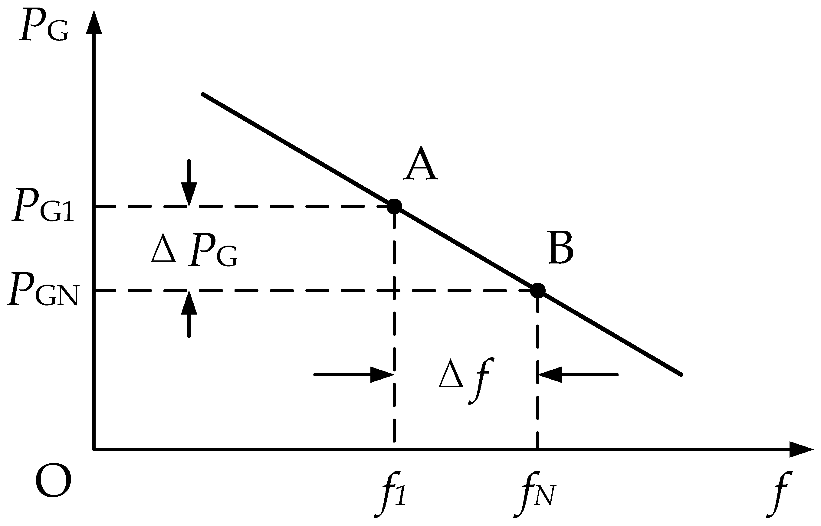
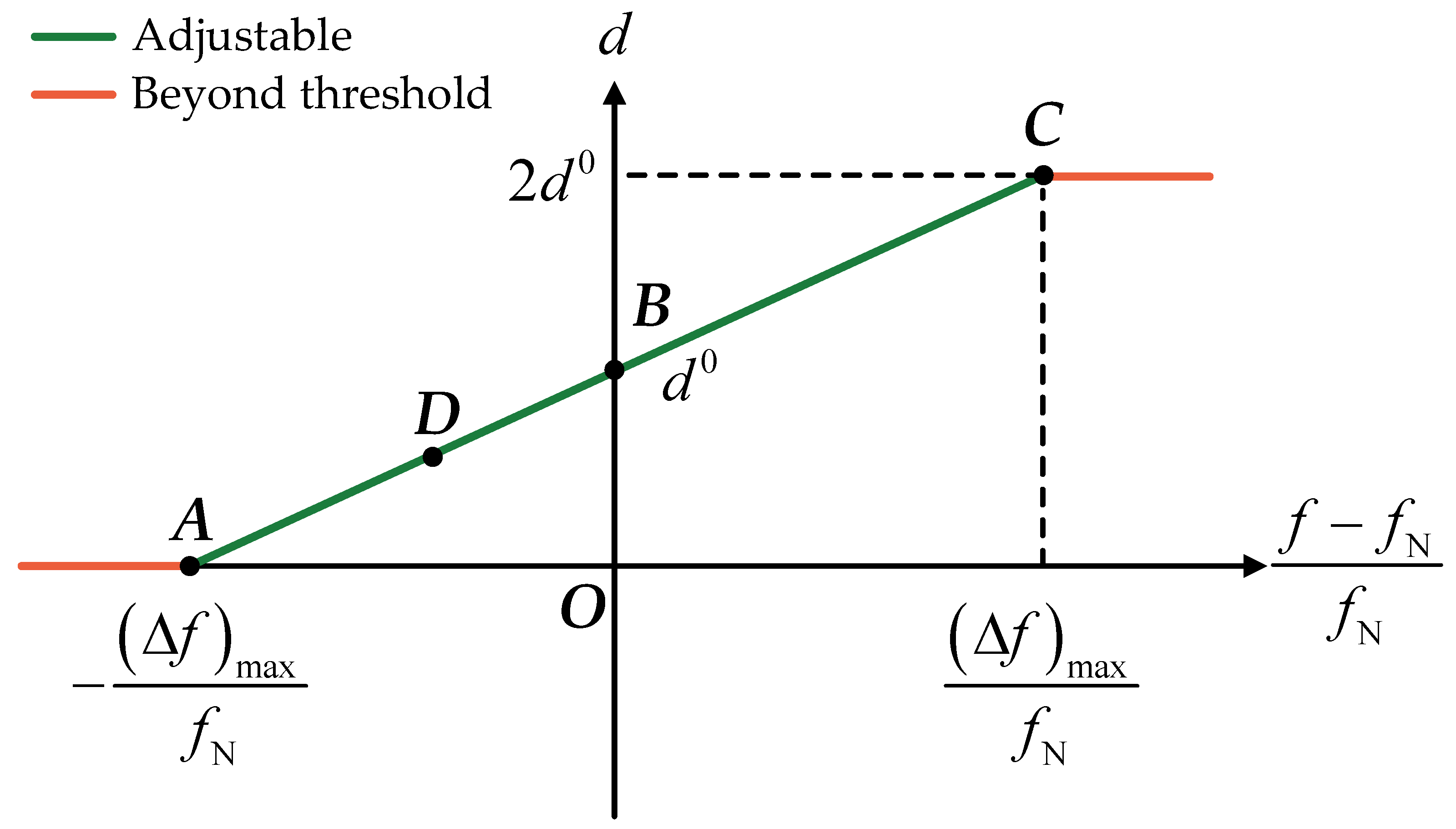
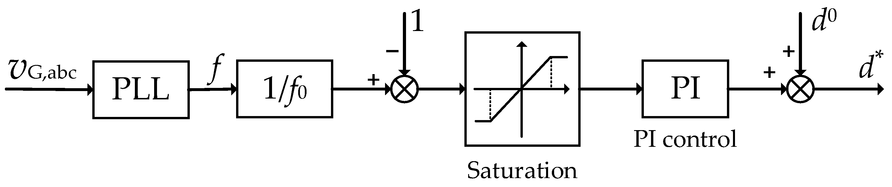
2.2. Determination Method of Power Reserve Ratio Based on the Frequency Response Module

Power imbalance is the primary reason for grid frequency deviation. To enable a PV system to participate in power system frequency regulation, it is essential to adjust its output power in real time based on the frequency deviation. Typically, to maximize the use of solar energy, a PV system is often controlled to operate at MPPs. However, when the microgrid frequency is lower than the standard frequency $f_{\mathrm{N}}$ and there is an urgent need to generate more power to alleviate power shortage, the PV system already running on MPPs cannot adjust its output power upwards. Therefore, the PV system participating in FR should reserve a portion of MAP when the grid frequency is $f_{\mathrm{N}}$, so as to cope with power shortages. Conversely, when the load decreases and the power overflow causes the frequency to increase, the PV system should correspondingly reduce the output power to minimize the frequency deviation of the microgrid.

This article introduces the power reserve ratio $d$ to describe the level of power generation of a PV system, which is defined as the percentage of the difference between the maximum power and actual power of the PV system and the maximum power ratio, as shown in Equation (7).

$$d=\frac{P_{\mathrm{d}\mathrm{e}}}{P_{\mathrm{m}}}=\frac{P_{\mathrm{m}}-P}{P_{\mathrm{m}}}$$

(7)

where $P_{\mathrm{m}}$ and $P$ are the maximum and actual output power of the PV system, respectively, and $P_{\mathrm{d}\mathrm{e}}$ is the reserved PV power.

Based on the analysis above, it is important to determine the initial power reserve ratio $d^0$ of the PV system when the grid frequency is stable at $f_{\mathrm{N}}$. If the initial power reserve ratio is too low, the PV system’s range of power variation in response to microgrid frequency fluctuations will be limited, resulting in suboptimal results for the participation of PV systems in FR. Conversely, if the initial power reserve ratio is too high, the power emitted by the PV system when the frequency deviation is zero will be far lower than MAP, leading to a waste of solar energy. Therefore, $d^0$ should be a parameter requiring sophisticated calculation, and the method for its value determination is explained in Section 3.3.

As shown in Figure 4, the curve represents the relationship between the frequency deviation rate and the power reserve ratio. Point B corresponds to the case where the microgrid frequency is at the standard frequency ($f=f_{\mathrm{N}}$), and the PV system should maintain a power reserve ratio of $d=d^0$. The PV power plant specifies the maximum frequency deviation that a PV system participating in frequency regulation can accept, recorded as $({∆f)}_{\mathrm{m}\mathrm{a}\mathrm{x}}$. If $f\in \left[f_{\mathrm{N}}-{(∆f)}_{\mathrm{m}\mathrm{a}\mathrm{x}},f_{\mathrm{N}}+({∆f)}_{\mathrm{m}\mathrm{a}\mathrm{x}}\right]$ is satisfied, the microgrid can be restored to the standard frequency using only the PV system; otherwise, extra approaches are required to assist with frequency regulation. Point A represents the case where the grid frequency is below the adjustable lower limit, i.e., $f<f_{\mathrm{N}}-({∆f)}_{\mathrm{m}\mathrm{a}\mathrm{x}}$, and the PV system should work at the MPP to output as much power as possible to alleviate the power shortage, so the power reserve ratio at point A is $d=0$. Similarly, the right side of point C corresponds to the circumstance where the frequency is higher than the adjustable upper limit, i.e., $f>f_{\mathrm{N}}+({∆f)}_{\mathrm{m}\mathrm{a}\mathrm{x}}$, and the output power of the PV system should be reduced. According to the linear relationship of the first-order function, the corresponding power reserve ratio at point C will be twice the initial power reserve ratio. The corresponding power at point C can be obtained by

$$P_{\mathrm{C}}=P_{\mathrm{m}}\left(1-2d^0\right)$$

(8)

It is evident that the y-intercept of this linear function is $d^0$, and its slope $k_{\mathrm{d}\mathrm{e}}$ can be expressed as follows:

$$k_{\mathrm{d}\mathrm{e}}=\frac{y_{\mathrm{A}}-y_{\mathrm{B}}}{x_{\mathrm{A}}-x_{\mathrm{B}}}=\frac{0-d^0}{-(∆{f)}_{\mathrm{m}\mathrm{a}\mathrm{x}}/f_{\mathrm{N}}-0}=\frac{f_{\mathrm{N}}}{(∆{f)}_{\mathrm{m}\mathrm{a}\mathrm{x}}}$$

(9)

Therefore, the functional expression of the curve of frequency deviation–power reserve ratio in Figure 4 is

$$d=\left\{\begin{array}{c}0,f<f_{\mathrm{N}}-({∆f)}_{\mathrm{m}\mathrm{a}\mathrm{x}}\\ k_{\mathrm{d}\mathrm{e}}\frac{f-f_{\mathrm{N}}}{f_{\mathrm{N}}}+d^0,f_{\mathrm{N}}-{(∆f)}_{\mathrm{m}\mathrm{a}\mathrm{x}}\le f\le f_{\mathrm{N}}+{(∆f)}_{\mathrm{m}\mathrm{a}\mathrm{x}}\\ 2d^0,f<f_{\mathrm{N}}+{(∆f)}_{\mathrm{m}\mathrm{a}\mathrm{x}}\end{array}\right.$$

(10)

P control is differential control, while PI control is zero differential control. If only P control is used here to achieve power reserve, although the frequency deviation will be greatly reduced, it still cannot bring the grid frequency back to the standard power frequency, so PI control should be used for adjustment. The control method shown in Figure 5 coordinates the application of PLL, which samples the frequency of the grid, a saturation module, which sets the threshold value of frequency deviation within the adjustable range, as well as PI control. Use the frequency of the collected grid-side voltage to calculate the target value $d^{\mathrm{*}}$ of the power reserve ratio of the PV system according to (10), so as to perform the remaining power reserve control. The parameters of PI control in the frequency response module are set as follows: $K_{\mathrm{p}}=55$ and $K_{\mathrm{i}}=12$.

2.3. Determination Method of BOOST Converter Duty Cycle Based on the Power Reserve Control Module

To ensure operational stability, PV systems are typically controlled to operate on the section of the P-V curve located on the right side of the MPP. It can be proved that the P-V curve on the right side of MPP monotonically decreases, and the derivative of P with respect to V also exhibits monotonicity for P. Therefore, each P value on the right side of MPP corresponds to a unique value of $(\mathrm{d}P/\mathrm{d}V)$, as depicted in Figure 6a. Equation (7) reveals that there is a linear relationship between the output power P and the power reserve ratio $d$ of the PV system. As a result, the derivative of P with respect to V must also have a one-to-one correspondence with the power reserve ratio $d$, as illustrated in Figure 6b, which is under the standard test condition (STC, $G=1000 \mathrm{W}/{\mathrm{m}}^2, T=25 °\mathrm{C}$).

Hence, Equation (11) can be employed to express the implicit function that relates $(\mathrm{d}P/\mathrm{d}V)$ to $d.$ By utilizing this function expression, the target value of $(\mathrm{d}P/\mathrm{d}V)$ can be obtained by substituting the target power reserve ratio $d^{\mathrm{*}}.$ The solution to the implicit function $h(·)$ is elaborated in Section 2.4.

$${(\frac{\mathrm{d}P}{\mathrm{d}V})}^{\mathrm{*}}=h(d^{\mathrm{*}})$$

(11)

If the PV system is controlled to operate at the target operating point on the P-V curve, where the tangent slope equals the target value ${(\mathrm{d}P/\mathrm{d}V)}^{*}$, the power reserve ratio of the operating point will reach the target value, i.e., $d=d^{*}.$ Since the frequency of the microgrid fluctuates, the target power reserve ratio $d^{*}$ also varies, and hence ${(\mathrm{d}P/\mathrm{d}V)}^{*}$ cannot be constant. To ensure the PV system operates at the target operating point, a parameter $k_{∆}\left(t\right)$ is defined as the difference between the tangent slope of the operating point and the target value. Therefore, we can express the parameter as

$$k_{∆}\left(t\right)=\left|\frac{∆P_{\mathrm{P}\mathrm{V}}\left(t\right)}{∆V_{\mathrm{P}\mathrm{V}}\left(t\right)}-{\left(\frac{\mathrm{d}P}{\mathrm{d}V}\right)}_t^{\mathrm{*}}\right|$$

(12)

where t is the current time stamp, $∆P_{\mathrm{P}\mathrm{V}}\left(t\right)=P_{\mathrm{P}\mathrm{V}}\left(t\right)-P_{\mathrm{P}\mathrm{V}}(t-1)$ represents the difference of PV power between the current and the last time stamp, and $∆V_{\mathrm{P}\mathrm{V}}\left(t\right)=V_{\mathrm{P}\mathrm{V}}\left(t\right)-V_{\mathrm{P}\mathrm{V}}(t-1)$ is that of PV voltage.

Before the commencement of the algorithm, certain parameters need to be preset, including the initial value $D\left(0\right)$, step-size $∆D,$ and initial change direction of duty cycle. It is worth mentioning that the choice of step size is crucial in determining the performance of operating point control. A small step size may lead to accurate tracking but may result in slow convergence and long computation time. On the other hand, a large step size may result in fast convergence but may lead to oscillations and instability. Therefore, a variable step-size strategy is preferred to balance the trade-off between accuracy and convergence speed. The variable step-size strategy for the BOOST converter is described in Section 3.2.

During the iteration, if $k_{∆}$ becomes larger than the previous value, the direction of movement of the duty cycle should be changed, and vice versa. The duty cycle is continuously adjusted until the target duty cycle $D^{\mathrm{*}}$ is reached, i.e., the change in $k_{∆}$ during the iteration is less than the preset threshold $\epsilon$. At this stage, the PV system operates at a point on the P-V curve where the tangent slope equals the target value ${(\mathrm{d}P/\mathrm{d}V)}^{*}$. Algorithm 1 presents the pseudocode of the power reserve control strategy.

Algorithm 1: Pseudocode of the power reserve control strategy

Set the initial value $D\left(0\right)$, step-size $∆D$, and initial change direction for duty cycle and the change threshold $\epsilon$

Set $t=0$, $k_{∆}\left(0\right)=0$, $k_{∆}\left(1\right)=+\infty$

while True do

$t=t+1$

if $\left|k_{∆}\left(t\right)-k_{∆}\left(t-1\right)\right|>\epsilon$ do

Sample $V_{PV}\left(t\right)$, $I_{PV}\left(t\right)$, $P_{PV}\left(t\right)=V_{PV}\left(t\right)\times I_{PV}\left(t\right)$

${∆P}_{PV}\left(t\right)=P_{PV}\left(t\right)-P_{PV}(t-1),$ ${∆V}_{PV}\left(t\right)=V_{PV}\left(t\right)-V_{PV}(t-1)$

Calculate $d^{*}\left(t\right)$ at time t by (10) and using the frequency response module presented in Figure 5

Obtain ${\left(\mathrm{d}\mathrm{P}/\mathrm{d}\mathrm{V}\right)}_{\mathrm{t}}^{\mathrm{*}}$ at time $t$ according to (11)

Calculate $k_{∆}\left(t\right)$ by (12)

if $k_{∆}\left(t\right)>k_{∆}\left(t-1\right)$ do

Make the adjustment direction of the duty cycle opposite: ${(∆D)}_t=-{(∆D)}_{t-1}$

else if $k_{∆}\left(t\right)\le k_{∆}\left(t-1\right)$ do

Keep the adjustment direction of the duty cycle: ${(∆D)}_t={(∆D)}_{t-1}$

end if

Adjust the duty cycle: $D\left(t\right)=D(t-1)+{(∆D)}_t$

end if

if the PV system no longer participates in microgrid frequency control do

break while

end if

end while

2.4. Solution of Function Expression of $(dP/dV)=h\left(d\right)$

Figure 6b depicts the functional relationship between $(\mathrm{d}P/\mathrm{d}V)$ and $d$, represented by $(\mathrm{d}P/\mathrm{d}V)=h\left(d\right)$, for a single PV module operating under STC. It is worth noting that this expression is dependent on environmental factors and the number of PV modules present in the system.

When the number of PV modules in the PV array changes, the function $h(·)$ will be scaled accordingly. The relationship between the function for the PV array composed of $n_{\mathrm{s}}$ modules connected in series and $n_{\mathrm{p}}$ modules connected in parallel and the functional expression of a single module is as follows:

$$\frac{\mathrm{d}{P}_{\mathrm{a}\mathrm{r}\mathrm{r}\mathrm{a}\mathrm{y}}}{\mathrm{d}{V}_{\mathrm{a}\mathrm{r}\mathrm{r}\mathrm{a}\mathrm{y}}}=\frac{\mathrm{d}\left(n_{\mathrm{s}}{n}_{\mathrm{p}}{P}_{\mathrm{m}\mathrm{o}\mathrm{d}\mathrm{u}\mathrm{l}\mathrm{e}}\right)}{\mathrm{d}\left(n_{\mathrm{s}}{P}_{\mathrm{m}\mathrm{o}\mathrm{d}\mathrm{u}\mathrm{l}\mathrm{e}}\right)}=\frac{n_{\mathrm{s}}{n}_{\mathrm{p}}}{n_{\mathrm{s}}}\frac{\mathrm{d}{P}_{\mathrm{m}\mathrm{o}\mathrm{d}\mathrm{u}\mathrm{l}\mathrm{e}}}{\mathrm{d}{V}_{\mathrm{m}\mathrm{o}\mathrm{d}\mathrm{u}\mathrm{l}\mathrm{e}}}=n_{\mathrm{p}}\frac{\mathrm{d}{P}_{\mathrm{m}\mathrm{o}\mathrm{d}\mathrm{u}\mathrm{l}\mathrm{e}}}{\mathrm{d}{V}_{\mathrm{m}\mathrm{o}\mathrm{d}\mathrm{u}\mathrm{l}\mathrm{e}}}$$

(13)

where $P_{module}$ and $V_{module}$ represent the power and voltage values of a PV module and $P_{array}$ and $V_{array}$ of a PV array composed of PV modules.

When changes occur in the external environment of the PV system, such as variations in irradiance intensity and cell temperature, the expression of the function $h(·)$ is also affected. The generally employed approach involves combining the mathematical model of PV array and (7) and using the Newton–Raphson method to obtain the expression of $h(·)$ through iterative process. An alternative and more efficient method is to develop a simplified PV cell model, which simplifies the mathematical model of PV array into a transcendental equation set comprising five equations and combines it with (7) to obtain the expression of $h(·)$. However, the former is limited by a long computational time owing to the continuous iterative solution of the transcendental equation, whereas the latter has a reduced computational accuracy, and even though it has improved computational efficiency, it still requires solving equations repeatedly at every moment. Therefore, a better approach is to use existing operating data efficiently for accurate and efficient fitting. Curve fitting using the least squares method is a data-driven approach to solving functional relationships, but inappropriate functional forms can lead to insufficient fitting accuracy or overfitting due to the unknown form of the simplified fitting expression. Thus, this study employs artificial neural networks (ANN) to fit the function $(\mathrm{d}P/\mathrm{d}V)=h\left(d\right)$, which can achieve higher accuracy and computational efficiency even without knowledge of the specific expression [26].

The structure of ANN is shown in Figure 7. In our problem, the values of $G$, $T,$ and $d$ are all able to influence the output value of $(\mathrm{d}P/\mathrm{d}V)=h\left(d\right)$. Therefore, $G$, $T$, and $d$ are set as the input of the ANN and the value of $(\mathrm{d}P/\mathrm{d}V)$ as the output.

The steps for solving the functional expression of $(\mathrm{d}P/\mathrm{d}V)=h\left(d\right)$ using ANN are as follows:

(i)

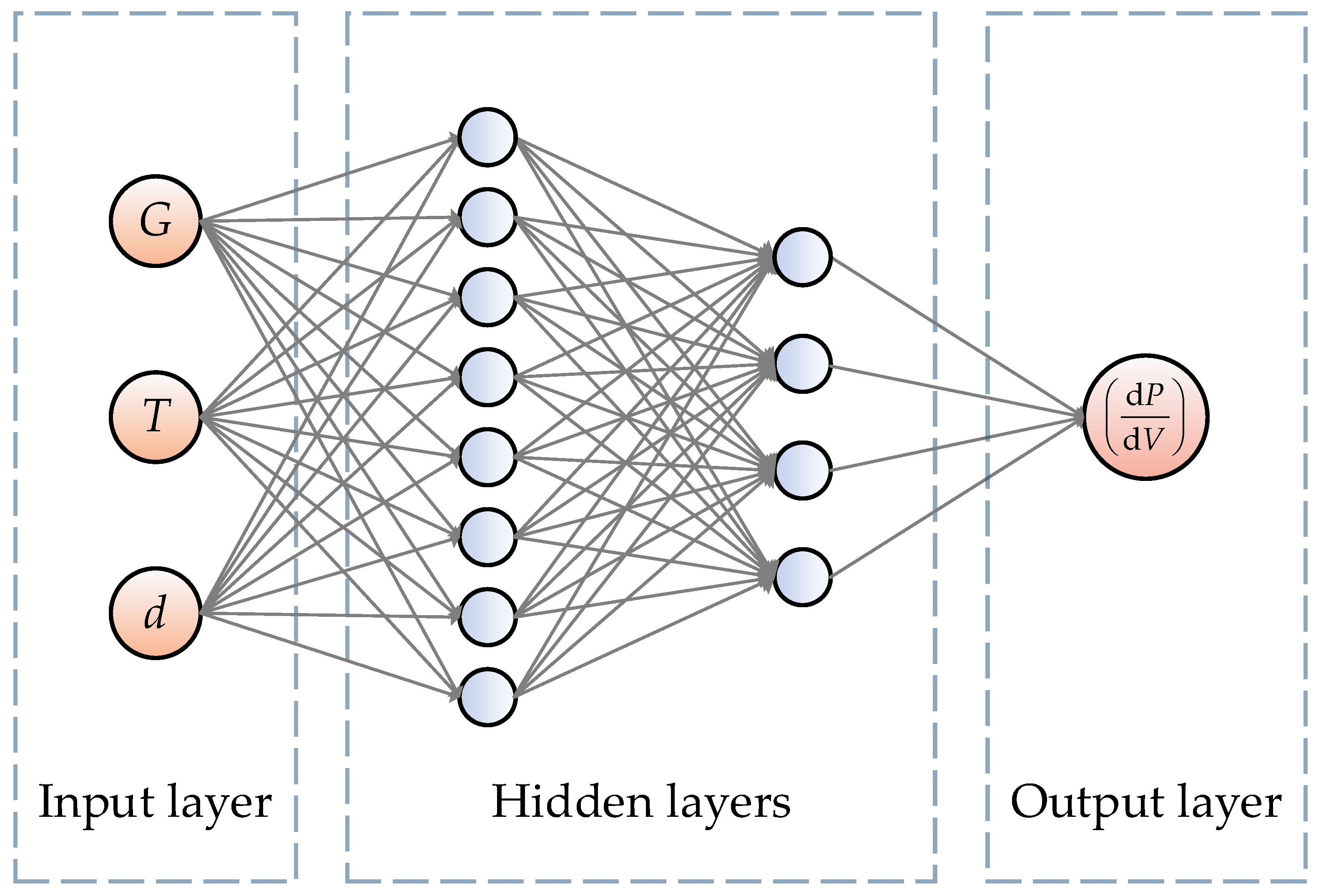
Set multiple combinations of irradiance intensity and cell temperature and test a single PV module under each combination, respectively. The duty cycle of the BOOST converter is continuously adjusted while collecting the following parameters of the PV module under each given external condition: power P, voltage V, and current $I$. The corresponding value of $(\mathrm{d}P/\mathrm{d}V)$ can be obtained by calculating $\mathsf{\Delta }P/\mathsf{\Delta }V,$ and $d$ can be calculated by (7). Thereby, numerous sets of $\left\{G,T,d,(\mathrm{d}P/\mathrm{d}V)\right\}$ are recorded as the sample dataset.

(ii)

Normalize the sample dataset by mapping it into $[0,1]$.

(iii)

Divide the sample dataset into training set, validation set, and test set by a ratio of 3:1:1.

(iv)

Obtain candidate ANN models with different hyperparameters using manual experience and grid search methods.

(v)

Train all candidate models on the training set.

(vi)

Evaluate the trained candidate models on the validation set and select the optimal ANN model.

(vii)

Test the optimal ANN model on the test set.

(vii)

Denormalize the output of the optimal ANN model to obtain the predictive values of $(\mathrm{d}P/\mathrm{d}V)$ and analyze them with some evaluation indicators.

(ix)

When a new set $\left\{G,T,d\right\}$ is given, the trained ANN model is used to calculate the corresponding $(\mathrm{d}P/\mathrm{d}V)$ of the PV module. The actual $(\mathrm{d}P/\mathrm{d}V)$ value of the whole PV array can be obtained by (13).

3. DRL-Based Strategies for Duty Cycle Variable Step-Size and Optimal Initial Power Reserve Ratio Selection

In Section 2, we presented a framework for integrating PV systems into the control strategy of microgrid frequency regulation. However, there are still two outstanding challenges that need to be addressed: (i) devising a step-size control strategy that facilitates rapid convergence of the PV system’s operating point to the target operating point, while ensuring accurate tracking after convergence; (ii) determining the optimal initial power reserve ratio that maximizes the utilization of solar energy while maintaining the frequency support capability of PV systems in microgrids. In this context, deep reinforcement learning (DRL) holds great promise in addressing these challenges, as it possesses exceptional decision-making capabilities that can be highly applicable in resolving these issues.

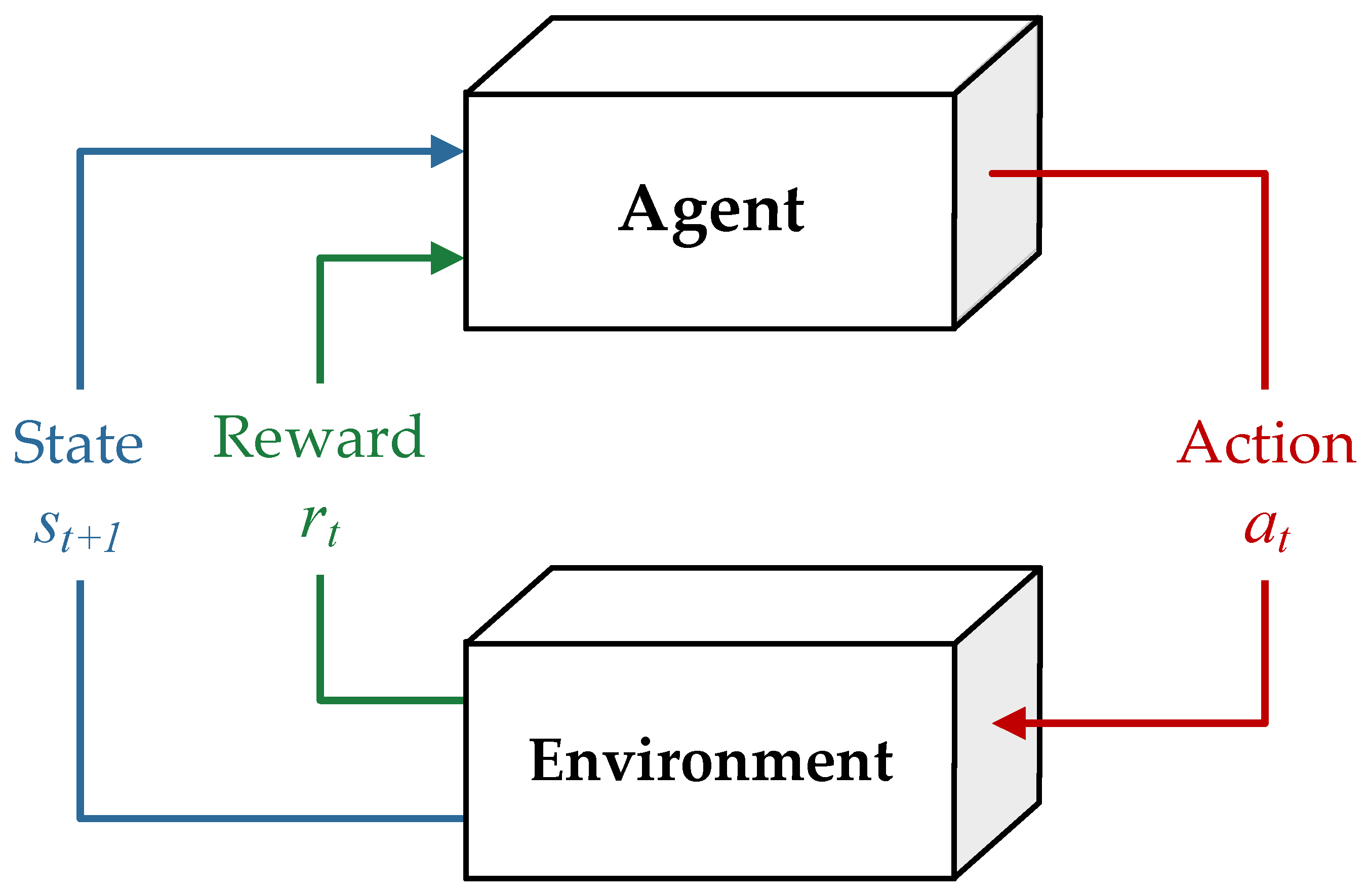
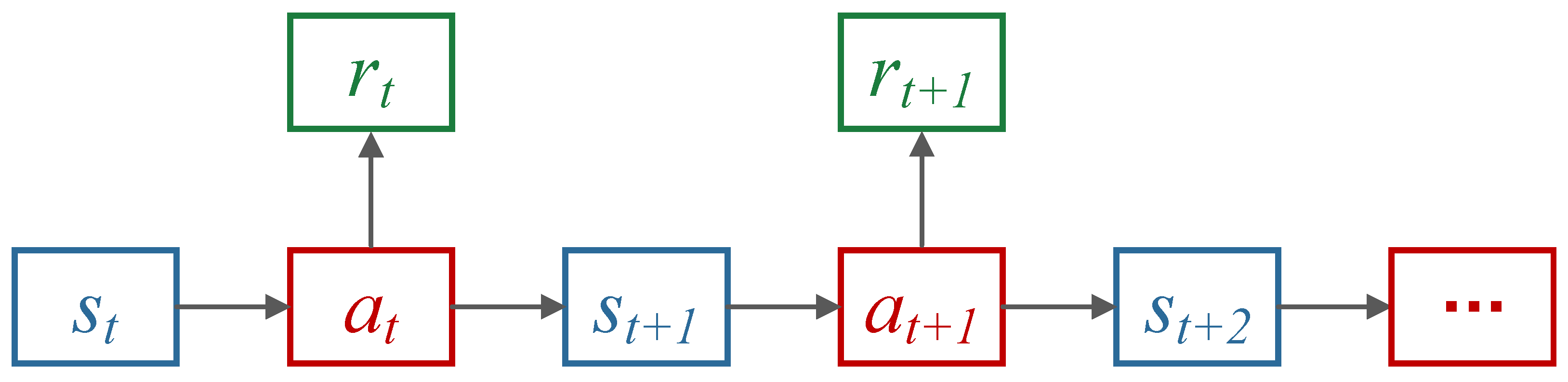
3.1. Fundamentals of Deep Reinforcement Learning

DRL is an algorithmic framework that models the mapping between environmental states and actions, with the ultimate objective of maximizing the cumulative reward that an agent receives through iterative trial-and-error interactions with a given environment [27].

The reinforcement learning framework comprises agents that can take a specific action $a_t$ based on the current state $s_t$, as depicted in Figure 8. Once an action is chosen at time $t$, the agent receives a scalar reward $r_{t+1}$ and transitions to a new state $s_{t+1}$, which is dependent on both the current state and the chosen action. The policy function $\pi (·)$ maps the agent’s current state to a specific action:

$$\pi \left(a_t|s_t\right)=\mathbb{P}\left(A=a_t|S=s_t\right)$$

(14)

where $A$ is the action variable referring to the entire set of possible actions that an agent can take in a given state, and $S$ represents the state variable, analogously.

The state transition function $p(·)$ characterizes the probability distribution of transitioning from one state to another under a specific action:

$$p\left(s_{t+1}|s_t,a_t\right)=\mathbb{P}(S^{\prime }=s_{t+1}|S=s_t,A=a_t)$$

(15)

As illustrated in Figure 9, the Markov decision process (MDP) adheres to the Markov property and serves as the fundamental formalism for reinforcement learning. It can be defined as follows:

$$p\left(s_{t+1}\right|s_0,a_0,s_1,a_1,\cdots ,s_t,a_t)=p(s_{t+1}|s_t,a_t)$$

(16)

During each epoch, the agent takes actions that modify its state within the environment and receives corresponding rewards. In order to better estimate the reward value, a value function and an optimal policy are introduced [27]. The aim is to maximize the long-term cumulative reward beyond the current time $t$ for a fixed time horizon that terminates at time $t$. This is expressed by the payoff $U_t$, as shown in Equation (17).

$$U_t=R_t+\gamma R_{t+1}+\gamma R_{t+2}+\cdots ={\sum }_{k=0}^{\infty }{\gamma }^k{R}_{t+k}$$

(17)

where $\gamma \in \left[0,1\right]$ is the discounted factor, a hyperparameter to be determined.

Various algorithms are utilized to determine the optimal policy, some of which involve utilizing an action-value function. The action-value function $Q_{\pi }(·)$ is utilized to represent the value of taking an action $a_t$ in a given state $s_t$ under a policy $\pi$ at time t, as demonstrated below:

$$Q_{\pi }(s_t,a_t)=\mathbb{E}\left[U_t\right|S=s_t,A=a_t]$$

(18)

Analogously, the state-value function $V_{\pi }(·)$ is indicative of how advantageous it is for the agent to reach a specific state $s_t$, and it is dependent on the agent’s current policy $\pi (·)$ [27], as shown in Equation (19).

$$V_{\pi }\left(s_t\right)={\mathbb{E}}_A\left[Q_{\pi }\right(s_t,A\left)\right]$$

(19)

where ${\mathbb{E}}_A(·)$ stands for the expectation for all actions.

In this article, deep Q-learning is adopted to find the optimal policy function. The Bellman equation can be utilized to express the Q-function iteratively in the Q-learning algorithm:

$$Q_{\pi }(s_t,a_t)=\mathbb{E}[R_{t+1}+\gamma Q_{\pi }(s_{t+1},a_{t+1}\left)\right|S=s_t,A=a_t]$$

(20)

The maximum cumulative reward can be achieved by selecting the optimal policy function ${\pi }^{*}(·)$, which leads to the optimal action-value function $Q^{*}(·)$, as demonstrated in Equation (21).

$$Q^{*}(s_t,a_t)=Q_{{\pi }^{*}}(s_t,a_t)={\mathrm{m}\mathrm{a}\mathrm{x}}_{\pi }{Q}_{\pi }(s_t,a_t)$$

(21)

where ${\mathrm{m}\mathrm{a}\mathrm{x}}_{\pi }(·)$ denotes the operation to obtain the maximum value by traversing all policy functions.

Then, the next optimal action for the agent based on the given new state $s_{t+1}$ is computed by

$$a_{t+1}={\mathrm{a}\mathrm{r}\mathrm{g}\mathrm{m}\mathrm{a}\mathrm{x}}_A{Q}^{*}(s_{t+1},A)$$

(22)

where ${\mathrm{a}\mathrm{r}\mathrm{g}\mathrm{m}\mathrm{a}\mathrm{x}}_A(·)$ denotes the operation to identify the optimal action $A$ from all possible actions to maximize the function value.

The optimization model presented in this paper involves nonlinear objectives and constraints. To tackle this challenge, we adopt deep Q-learning [28], which leverages the power of deep neural networks and reinforcement learning to process large-scale data effectively. This approach enables agent training using vast amounts of data, leading to real-time decision making based on the current state variables and ultimately resulting in optimal parameter setting. Specifically, the state vector $S$ is used as the input sequence through the neural network, and the approximated $Q_{\pi }(·)$ is obtained in the output layer. The network consists of h hidden layers, each composed of u neurons, where h and u are hyperparameters determined by the specific calculation example. In this study, the neural network comprises four hidden layers, and the activation function used is ReLU (rectified linear unit).

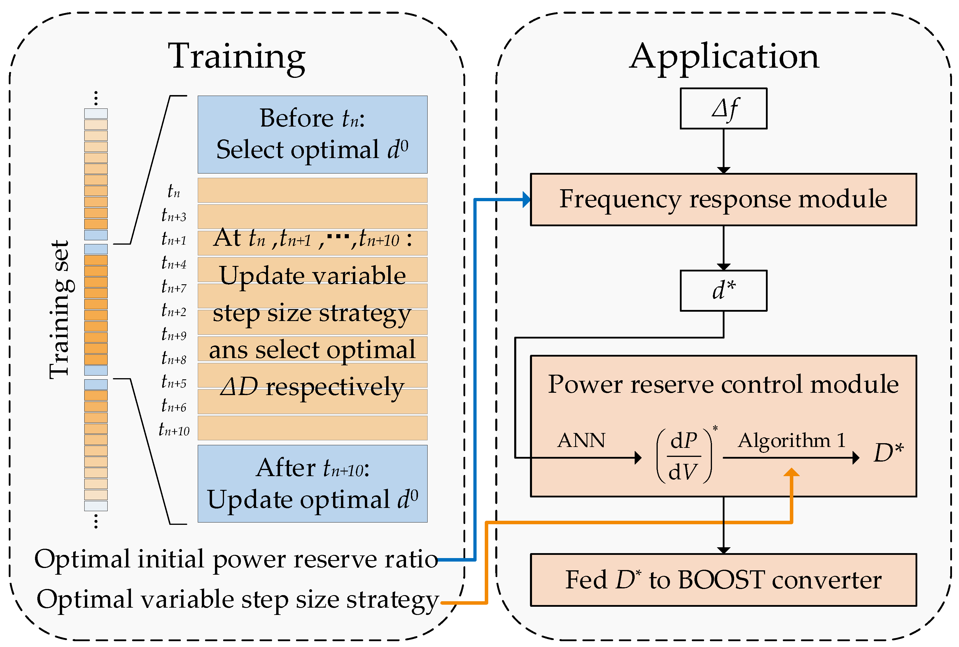
3.2. DRL-Based Optimal Strategy for Duty Cycle with Variable Step Sizes

According to Section 2.3, where the determination method of the BOOST converter duty cycle based on the power reserve control module was introduced, the choice of duty cycle step size is crucial in determining the performance of the power reserve control algorithm. Using a small step size can achieve accurate tracking, but it comes at the cost of slow convergence and prolonged computation time. Conversely, a large step size can lead to fast convergence, but it may result in oscillations and instability. Consequently, a variable step-size strategy is deemed preferable to balance the trade-off between accuracy and convergence speed.

One common approach to variable step size is to use a variable step size that changes with the PV system’s operating conditions [22]. The variable step size is typically proportional to the change in the PV array’s output power or voltage. Specifically, a large step size is used when the PV array is far from the target operating point, and a small step size is used when the PV array is close to it. This strategy ensures adequate convergence speed and better accuracy and avoids overshooting and oscillations. However, the general variable step-size strategy has some limitations, such as inflexible adjustment time, which can lead to suboptimal performance under changing external conditions, and finite available step sizes, causing limited adjustment accuracy. The aforementioned limitations can have a detrimental impact on the ability to track the desired power reserve ratio, ultimately leading to a reduction in the overall performance of microgrid frequency regulation. In contrast, using DRL can effectively overcome these limitations and provide more flexible and optimized step-size decisions.

To determine the variable step size of the BOOST converter, the state variables should include the irradiance intensity, the cell temperature, the frequency deviation, the target power reserve ratio, the operating current and voltage of the PV array, the current and last duty cycle step sizes, and the current time stamp. Therefore, the state space can be expressed as

$$S=[G(t),T(t),{(∆f)}_t,{{(d}^{*})}_t,{I_{\mathrm{P}\mathrm{V}}(t),V_{\mathrm{P}\mathrm{V}}(t),(∆D)}_t,{(∆D)}_{t-1},t]$$

(23)

The action variable is referred to as the change in the duty cycle step size, so the action space is

$$A={\left({∆}^{2}D\right)}_t$$

(24)

where ${\left({∆}^{2}D\right)}_t$ is the change in the duty cycle step size. The duty cycle step size at the next time stamp is determined by ${{(∆D)}_{t+1}={(∆D)}_t+\left({∆}^{2}D\right)}_t$.

The aim of optimizing the variable step size of the BOOST converter using DRL is to minimize the cumulative frequency deviation through an optimal action-value function $Q^{*}(·)$ learned by the agent. The performance of a given variable step-size strategy is negatively impacted as the cumulative frequency deviation grows larger. To address this, the problem is reformulated as a reward maximization task in the DRL framework. As a result, the agent’s reward function can be expressed as

$$R=-{(∆f)}_t$$

(25)

3.3. DRL-Based Optimal Strategy for Initial Power Reserve Ratio Selection

According to Section 2.2, where the determination method of power reserve ratio based on frequency response module was introduced, the selection of the initial power reserve ratio significantly affects the efficacy of the power reserve control algorithm. The initial power reserve ratio plays a crucial role in determining the level of PV system involvement in the FR of the microgrid, as well as the portion of solar energy wasted. It is essential to select the optimal initial power reserve ratio, taking into account both the frequency support ability of the PV system for the microgrid and the utilization rate of solar energy.

Similar to Section 3.2, the state space and the action space can be expressed using Equations (26) and (27):

$$S=[G(t),T(t),{(∆f)}_t,{{(d}^{*})}_t,MAP\left(t\right),P_{\mathrm{P}\mathrm{V}}(t),t]$$

(26)

$$A=d^0$$

(27)

The agent’s reward function can be defined as

$$R=-\left[\frac{{(∆f)}_t}{{(∆f)}_{max}}+\frac{MAP\left(t\right)-P_{\mathrm{P}\mathrm{V}}\left(t\right)}{MAP\left(t\right)}\right]$$

(28)

where ${(∆f)}_{max}$ is the maximum frequency deviation allowed in the microgrid and $MAP\left(t\right)$ is the maximum available power of the PV system at time $t$. ${(∆f)}_t/{(∆f)}_{max}$ denotes the frequency deviation cost, indicating the extent of frequency deviation at time $t$. $[MAP\left(t\right)-P_{\mathrm{P}\mathrm{V}}(t\left)\right]/MAP\left(t\right)$, also denoted as the power wastage cost, represents the degree of solar energy wastage at time $t$. To make these costs dimensionless, both are normalized using their own denominators. The selection of the optimal initial power reserve ratio should take into account both costs, with the aim of minimizing their sum. This requires a comprehensive evaluation of both factors, and the agent’s reward function is thereby maximized.

In the strategy training process, the optimization of the variable step-size strategy is performed at each time stamp, whereas the optimization of the initial power reserve ratio selection strategy is carried out every ten time stamps. Thereby, the proposed AI-based control strategy for PV systems participating in the FR of a microgrid can be illustrated as shown in Figure 10. The training process involves using DRL to obtain the optimal strategies of power reserve ratio selection and variable duty cycle step size. Subsequently, the obtained parameters are applied to the power reserve control algorithm, as discussed in Section 2, to enhance the system’s performance.

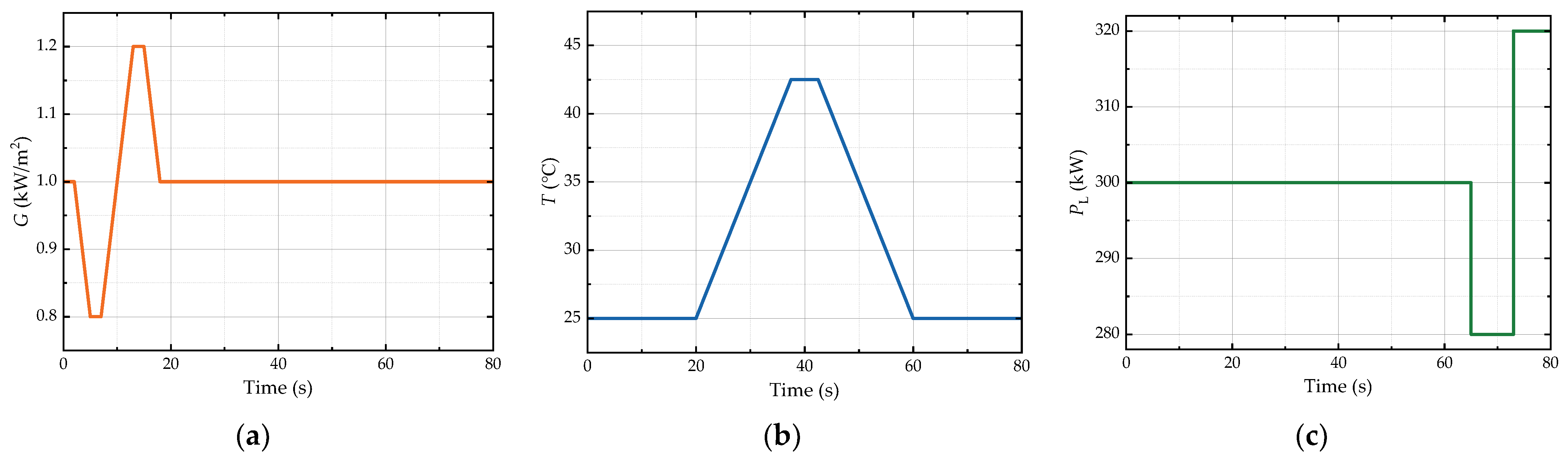
4. Simulation Verification

To validate the effectiveness of the proposed control strategy for PV systems participating in FR, we conducted three sets of simulations. The first set examined the ability of the power reserve control module, which utilizes ANN, in tracking a given power reserve ratio, and we compared its performance with other methods. The second set compared the performance of the proposed DRL-based duty cycle variable step-size strategy with some other step-size selection methods. The last set evaluated the effect of the initial power reserve ratio determined using DRL, as well as the overall performance of the proposed frequency regulation strategy for the PV system.

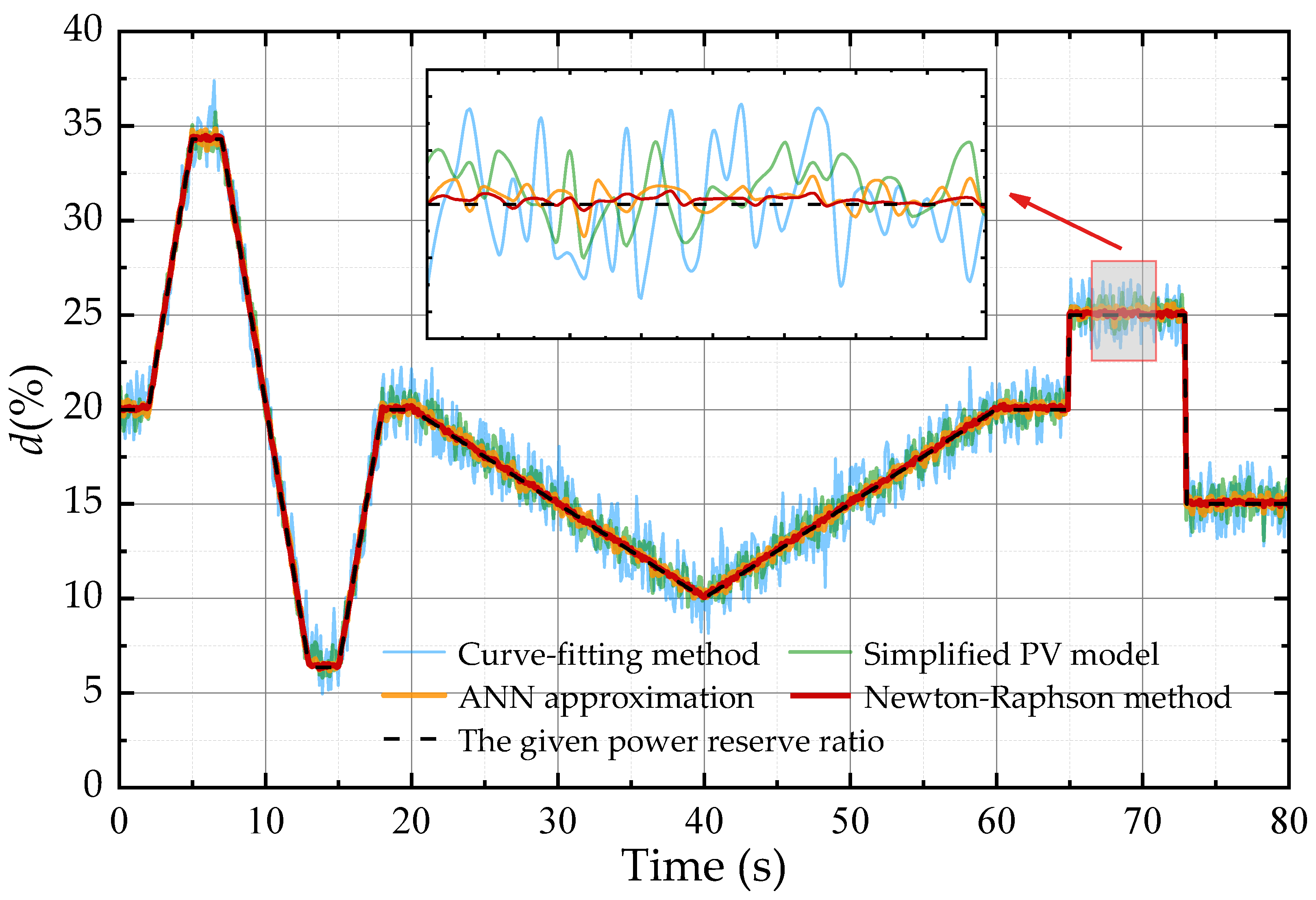
4.1. Case 1: Evaluation of Power Reserve Control Module Using Different Methods

The accuracy and efficiency of different solution methods for tracking the target power reserve ratio play a crucial role in determining the sensitivity and performance of the power reserve control module. To this end, the expression for $(\mathrm{d}P/\mathrm{d}V)=h\left(d\right)$ must be solved in the power reserve control module to allow for the calculation of ${(\mathrm{d}P/\mathrm{d}V)}^{\mathrm{*}}$ based on $d^{\mathrm{*}}$ when a target power reserve ratio is given. This enables the input of the corresponding duty cycle $D^{\mathrm{*}}$ into the BOOST converter. In this case, the irradiance intensity and cell temperature were given, as shown in Figure 11a,b, and the curve of the given power reserve ratio was also provided, as shown in Figure 12.

To evaluate the sensitivity of different solution methods in tracking $d^{\mathrm{*}}$, we employed the curve-fitting method proposed in [20], a simplified PV model utilized in [21], the ANN approximation method proposed in this study, and the Newton–Raphson method used in [22], respectively. The structure of the ANN is shown in Figure 7, having two hidden layers with eight and four neurons, respectively. The relevant parameters of the PV array are shown in

Table A1. Parameters in the mathematical model for the solar PV array [29].

Symbol	Parameter Name	Value	Unit
$q$	The electron charge	$1.60\times {10}^{-19}$	$\mathrm{C}$
$k$	The Boltzman constant	$1.38\times {10}^{-23}$	$\mathrm{J}/\mathrm{K}$
$A$	The ideality factor	1.72	-
$K_{\mathrm{i}}$	The temperature coefficient	$1.70\times {10}^{-3}$	$\mathrm{A}/\mathrm{K}$
$G$	The irradiance	Given	$\mathrm{W}/{\mathrm{m}}^2$
$T_{\mathrm{a}}$	The ambient temperature	Given	$\mathrm{K}$
$T_{\mathrm{r}}$	The reference temperature	298.15	$\mathrm{K}$
$T_{\mathrm{c}}\left(T\right)$	The cell temperature	$T_{\mathrm{a}}+0.028G-1$	$\mathrm{K}$
$I_{\mathrm{s}\mathrm{c}\mathrm{r}}$	The reference short circuit current at $T_{\mathrm{r}}$	3.30	$\mathrm{A}$
$I_{\mathrm{s}\mathrm{c}}$	The short circuit current	$G\left[I_{\mathrm{s}\mathrm{c}\mathrm{r}}+K_{\mathrm{i}}\left(T_{\mathrm{c}}-T_{\mathrm{r}}\right)\right]$	A
$I_{\mathrm{o}\mathrm{r}}$	The reverse current at $T_{\mathrm{r}}$	$19.97\times {10}^{-6}$	$\mathrm{A}$
$I_{\mathrm{s}}$	The diode saturation current	$I_{\mathrm{o}\mathrm{r}}{\left(T_{\mathrm{c}}/T_{\mathrm{r}}\right)}^3{\times \mathrm{e}}^{q{E}_g\left(1/T_{\mathrm{r}}-1/T_{\mathrm{c}}\right)/\left(kA\right)}$	$\mathrm{A}$
$R_{\mathrm{s}\mathrm{h}}$	The shunt resistance	313.40	$\mathsf{\Omega }$
$R_{\mathrm{s}}$	The series resistance	0.39	$\mathsf{\Omega }$
$n_{\mathrm{p}}$	The number of cells in parallel	9	-
$n_{\mathrm{s}}$	The number of cells in series	21	-

, and the duty cycle step size was temporarily set to 0.05. The measured power reserve ratio by different tracking methods were obtained by (7). Figure 12 shows the effect of the power reserve control modules based on different methods of tracking $d^{\mathrm{*}}$.

From the results shown in Figure 12, it can be observed that using the Newton–Raphson method to solve $(\mathrm{d}P/\mathrm{d}V)=h\left(d\right)$ for the power reserve control module exhibits the best tracking control effect on the power reserve ratio, with results almost consistent with the given power reserve ratio. On the other hand, using the ANN approximation, simplified PV model, and curve-fitting method exhibits a descending order of tracking performance. However, the Newton–Raphson method’s high accuracy comes at the cost of relatively complex iterative processes and long calculation times. Under severe fluctuations of external conditions and load, this method may not be able to track the target power reserve ratio promptly, leading to a decrease in frequency regulation performance. Therefore, when evaluating the effects of different methods used in power reserve control, it is necessary to comprehensively consider the accuracy of tracking the target power reserve ratio, which can be characterized by the root mean square error (RMSE) between the given power reserve ratio and the measured one, as well as the calculation time of different methods, as shown in

Table 1. Effects of different methods used in power reserve control strategy.

Method	RMSE		Calculation Time		Total Reduction
	Value (%)	Reduction (%)	Value (ms)	Reduction (%)	Value (%)	Ranking
Curve-fitting method	1.28	0	38.46	86.68	86.68	4
Simplified PV model	0.63	50.78	33.47	88.40	139.18	2
ANN approximation	0.26	79.68	43.87	84.80	164.48	1
Newton–Raphson method	0.12	90.63	288.64	0	90.63	3

Note: For RMSE reduction, the benchmark is “curve-fitting method”, and for calculation time reduction, the benchmark is “Newton–Raphson method”. The value of total reduction is the sum of RMSE reduction and calculation time reduction.

.

Table 1 shows that the performance of the ANN approximation method surpassed the power reserve control methods tested to different degrees, considering both the accuracy and speed of tracking a given $d^{\mathrm{*}}$. Therefore, in the subsequent simulations, the ANN approximation method was used in the power reserve control module.

4.2. Case 2: Evaluation of DRL-Based Duty Cycle Variable Step-Size Strategy

As discussed in Section 3.2, the conventional approach of determining the duty cycle step size for the power reserve control strategy has notable limitations. The variable step-size method proposed by [10] takes into consideration both convergence speed and stability accuracy, making it a better alternative to the fixed step-size method. However, whether it involves selecting a disturbance step size from a set of available step sizes or introducing a scaling coefficient to compress the step size, these methods have shown satisfactory results in MPPT algorithms but still have significant room for improvement when dealing with FR scenarios with external environmental and load fluctuations. Therefore, this case study aims to compare the frequency stabilization effects of three control strategies under various external disturbance conditions in the microgrid: MPPT control, power reserve control based on the variable step-size algorithm proposed by [10], and power reserve control using the variable step-size strategy proposed in this paper.

In this case, a simplified microgrid model was used, which consisted of a PV system, a synchronous generator, and a load, as shown in Figure 1. The standard frequency of the microgrid was 50 Hz. The MPP of the PV system under STC was set to 100 kW, and its relevant parameters were shown in Table A1. The synchronous generator was a diesel generator with an initial power output of 200 kW, and its parameters are presented in

Table A2. Parameters of the thermal synchronous generator.

Symbol	Parameter Name	Value	Unit
$P_{\mathrm{c}}$	Total capacity	3	MW
$k_{\mathrm{d}}$	Droop coefficient	15	$-$
$T_{\mathrm{g}}$	Governor time constant	0.2	-
$F_{\mathrm{r}}$	Reheat coefficient	5	-
$T_{\mathrm{r}}$	Reheat time constant	0.2	-
$T_{\mathrm{t}}$	Turbine time constant	0.2	-
$H$	Rotor inertia constant	4	-
$D$	Damping coefficient	1	$-$
$f_{\mathrm{n}}$	Standard frequency	50	Hz

. The load had an initial power of 300 kW. The fluctuation of external environment and load is shown in Figure 11, and the initial power reserve ratio was set to 20%. Additionally, the hyperparameters of the deep Q-learning agent for the power reserve control system are set as follows: the discount factor $\gamma$ was 0.9, the data sampling size was 256, the experience pool size was 106, the network parameter learning rate $\alpha$ was 0.0001, and the Adam optimizer was used to update the network weights. The simulation platform employed Python software and a i5-8250U computing unit to construct and validate the simulation model.

Figure 13 presents the simulation results. Initially, when only the synchronous generator participated in FR, the frequency fluctuation of the microgrid was high. Then, the power reserve control strategy proposed in this article was applied to the PV system to achieve FR. The variable step-size FR strategy proposed by [10] was employed, resulting in a significant reduction in frequency fluctuation, as evidenced by the area of the blue shaded portion in Figure 13. Subsequently, the DRL-based variable step-size FR strategy proposed in this article was used, which led to a further decrease in frequency fluctuation, as indicated by the area of the green shaded portion.

Upon analysis, it was observed that when the PV system did not participate in FR, the average frequency deviation was 0.0809 Hz. After employing the variable step-size FR strategy proposed by [10], the frequency deviation decreased by an average of 0.0301 Hz, which is a 62.87% reduction compared with the previous case. Furthermore, the frequency deviation decreased by an additional average of 0.0224 Hz, which represents a reduction of 9.49% and 72.36%, respectively, compared with the previous cases where the variable step-size FR strategy proposed by [10] and the PV system were not involved in FR, respectively.

These results demonstrate the efficacy of the power reserve frequency regulation control using the DRL-based variable step-size strategy proposed in this article, and this variable step-size strategy is used in the next set of simulations.

4.3. Case 3: Evaluation of DRL-Based Optimal Power Reserve Ratio Selection Strategy

Based on the discussion in Section 3.3, the initial power reserve ratio is a critical factor that determines the extent to which PV systems can participate in the FR of a microgrid, as well as the portion of wasted solar energy. The optimal initial power reserve ratio should consider both the frequency support ability of the PV system for the microgrid and the utilization rate of solar energy. However, manual experience is often used to determine the initial power reserve ratio, meaning that it is selected from a limited set of candidate numbers, resulting in a deviation from the optimal value and a limit to the capacity of the PV system to provide maximum frequency support or to achieve optimal solar energy utilization.

In this case, the irradiance intensity curve and load power curve were provided with a random fluctuation, as depicted in Figure 14, while the cell temperature was maintained at 25 °C. The allowed maximum frequency deviation was $∆f=0.2 \mathrm{H}\mathrm{z}$.

In the first step, we simulated the selection of initial power reserve ratio using manual experience. The value of the initial power reserve ratio $d^0$ was varied from 0% to 50% in 5% intervals. The cost of frequency deviation and power waste were calculated based on simulated operating data for each value of $d^0$. The costs were then added to obtain a cost function value for a limited number of power reserve ratios. The cost function value is shown in Figure 15. The optimal initial power reserve ratio was determined to be 25%, with the corresponding frequency deviation cost, power waste cost, and total cost being 15.56%, 24.98%, and 40.62%, respectively.

Subsequently, the proposed DRL-based optimal initial power reserve ratio selection strategy was employed to facilitate the participation of the PV system in the FR of the microgrid. The optimized initial power reserve ratio was determined to be 23.14%, which resulted in a frequency deviation cost of 16.11%, a power waste cost of 23.14%, and a total cost of 39.25%. It is noteworthy that the total cost is lower than that of the initial power reserve ratio selected through manual experience. Compared with the selection method based on manual experience, which may suffer from extensive interval division and incorrect judgment in worse scenarios, the DRL-based optimal initial power reserve ratio selection strategy provides superior performance in terms of the ability to participate in the FR of the microgrid.

5. Conclusions

This study proposed a novel AI-based power reserve control strategy for PV systems participating in the FR of microgrids, which overcomes the limitations of traditional methods based on accurate mathematical equations or simplified PV models. The proposed strategy starts by collecting the frequency deviation of the microgrid and uses a frequency response module to determine the target power reserve ratio of the PV system. Then, a power reserve control module is employed to obtain the target duty cycle, which is fed to the BOOST converter to control the PV operating point. The proposed control strategy enables the PV system to work at a specified power reserve ratio, producing appropriate power to mitigate frequency fluctuations in the microgrid.

The effectiveness of the proposed method was validated through simulations, highlighting its potential for practical applications in real-world microgrids. The results show that the ANN approximation outperformed other methods in the power reserve control module for target PV operating point tracking. Moreover, the proposed DRL-based strategy for variable step size surpassed the conventional method in reducing frequency deviations by 73.36% and 62.87%, respectively, when facing fluctuations in the external environment and load. Additionally, the use of DRL for the selection of the optimal initial power reserve ratio outperformed the use of manual experience in terms of the integrated degree of frequency deviation and solar energy wastage. Overall, the AI-based power reserve control strategy for PV systems participating in the FR of a microgrid demonstrated satisfactory performance in reducing frequency deviation, which is crucial for improving the frequency support capacity of PV systems, promoting the absorption of new energy led by PV systems, and reducing the phenomenon of light abandonment.

References

1. Liu, J.; Han, X.; Wang, L.; Zhang, P.; Wang, J. Operation and Control Strategy of DC Microgrid. Power Syst. Technol. 2014, 38, 2356–2362. [Google Scholar]
2. Saidi, A.S. Impact of large photovoltaic power penetration on the voltage regulation and dynamic performance of the Tunisian power system. Energy Explor. Exploit. 2020, 38, 1774–1809. [Google Scholar] [CrossRef]
3. Zhang, J.F.; Li, N.; Liu, J. A peaking-regulation-balance-based method for wind & PV power integrated accommodation. In Proceedings of the 2nd International Conference on Energy Engineering and Environmental Protection (EEEP), Sanya, China, 20–22 November 2017. [Google Scholar]
4. Yang, B.; Wang, X.; Xie, D.; Guo, Y. Novel control strategy of grid-connected photovoltaic power supply for frequency regulation. J. Eng. 2019, 2019, 1488–1491. [Google Scholar] [CrossRef]
5. Xin, H.; Liu, Y.; Wang, Z.; Gan, D.; Yang, T. A New Frequency Regulation Strategy for Photovoltaic Systems Without Energy Storage. IEEE Trans. Sustain. Energy 2013, 4, 985–993. [Google Scholar] [CrossRef]
6. Khazaei, J.; Tu, Z.; Liu, W. Small-Signal Modeling and Analysis of Virtual Inertia-Based PV Systems. IEEE Trans. Energy Convers. 2020, 35, 1129–1138. [Google Scholar] [CrossRef]
7. Neely, J.; Johnson, J.; Delhotal, J.; Gonzalez, S.; Lave, M. Evaluation of PV Frequency-Watt Function for Fast Frequency Reserves. In Proceedings of the 31st Annual IEEE Applied Power Electronics Conference and Exposition (APEC), Long Beach, CA, USA, 20–24 March 2016; pp. 1926–1933. [Google Scholar]
8. Li, H.J.; Xu, Y.; Adhikari, S.; Rizy, D.T.; Li, F.X.; Irminger, P. Real and Reactive Power Control of a Three-Phase Single-Stage PV System and PV Voltage Stability. In Proceedings of the General Meeting of the IEEE-Power-and-Energy-Society, San Diego, CA, USA, 22–26 July 2012. [Google Scholar]
9. Yan, G.G.; Liang, S.; Jia, Q.; Cai, Y.R. Novel adapted de-loading control strategy for PV generation participating in grid frequency regulation. J. Eng. 2019, 2019, 3383–3387. [Google Scholar] [CrossRef]
10. Zhong, C.; Zhou, Y.; Yan, G.G. Power reserve control with real-time iterative estimation for PV system participation in frequency regulation. Int. J. Electr. Power Energy Syst. 2021, 124, 106367. [Google Scholar] [CrossRef]
11. Shim, J.W.; Verbic, G.; Zhang, N.; Hur, K. Harmonious Integration of Faster-Acting Energy Storage Systems Into Frequency Control Reserves in Power Grid With High Renewable Generation. IEEE Trans. Power Syst. 2018, 33, 6193–6205. [Google Scholar] [CrossRef]
12. Bullich-Massague, E.; Aragues-Penalba, M.; Sumper, A.; Boix-Aragones, O. Active power control in a hybrid PV-storage power plant for frequency support. Sol. Energy 2017, 144, 49–62. [Google Scholar] [CrossRef]
13. Shi, R.L.; Zhang, X. VSG-Based Dynamic Frequency Support Control for Autonomous PV-Diesel Microgrids. Energies 2018, 11, 1814. [Google Scholar] [CrossRef]
14. Quan, X.J.; Yu, R.Y.; Zhao, X.; Lei, Y.; Chen, T.X.; Li, C.J.; Huang, A.Q. Photovoltaic Synchronous Generator: Architecture and Control Strategy for a Grid-Forming PV Energy System. IEEE J. Emerg. Sel. Top. Power Electron. 2020, 8, 936–948. [Google Scholar] [CrossRef]
15. Tarraso, A.; Candela, J.I.; Rocabert, J.; Rodriguez, P. Synchronous Power Control for PV Solar Inverters With Power Reserve Capability. In Proceedings of the 43rd Annual Conference of the IEEE-Industrial-Electronics-Society (IECON), Beijing, China, 29 October–1 November 2017; pp. 2712–2717. [Google Scholar]
16. Sangwongwanich, A.; Yang, Y.H.; Blaabjerg, F.; Sera, D. Delta Power Control Strategy for Multistring Grid-Connected PV Inverters. IEEE Trans. Ind. Appl. 2017, 53, 3862–3870. [Google Scholar] [CrossRef]
17. Sangwongwanich, A.; Yang, Y.H.; Blaabjerg, F. A Sensorless Power Reserve Control Strategy for Two-Stage Grid-Connected PV Systems. IEEE Trans. Power Electron. 2017, 32, 8559–8569. [Google Scholar] [CrossRef]
18. Li, N.; Liang, J.; Zhao, Y. Research on Dynamic Modeling and Stability of Grid-connected Photovoltaic Power Station. Proc. Chin. Soc. Electr. Eng. 2011, 31, 12–18. [Google Scholar]
19. Zarina, P.P.; Mishra, S.; Sekhar, P.C. Exploring frequency control capability of a PV system in a hybrid PV-rotating machine-without storage system. Int. J. Electr. Power Energy Syst. 2014, 60, 258–267. [Google Scholar] [CrossRef]
20. Rajan, R.; Fernandez, F.M. Power control strategy of photovoltaic plants for frequency regulation in a hybrid power system. Int. J. Electr. Power Energy Syst. 2019, 110, 171–183. [Google Scholar] [CrossRef]
21. Liao, S.Y.; Xu, J.; Sun, Y.Z.; Bao, Y.; Tang, B.W. Wide-area measurement system-based online calculation method of PV systems de-loaded margin for frequency regulation in isolated power systems. IET Renew. Power Gener. 2018, 12, 335–341. [Google Scholar] [CrossRef]
22. Batzelis, E.I.; Kampitsis, G.E.; Papathanassiou, S.A. Power Reserves Control for PV Systems With Real-Time MPP Estimation via Curve Fitting. IEEE Trans. Sustain. Energy 2017, 8, 1269–1280. [Google Scholar] [CrossRef]
23. Yan, R.F.; Saha, T.K.; Modi, N.; Masood, N.A.; Mosadeghy, M. The combined effects of high penetration of wind and PV on power system frequency response. Appl. Energy 2015, 145, 320–330. [Google Scholar] [CrossRef]
24. Banshwar, A.; Sharma, N.K.; Sood, Y.R.; Shrivastava, R. Renewable energy sources as a new participant in ancillary service markets. Energy Strateg. Rev. 2017, 18, 106–120. [Google Scholar] [CrossRef]
25. Li, D.; Chen, S.; Chen, Z.; Lu, J. Real-time measurement and reward method of the efficiency of generator unit primary frequency regulation. Autom. Electr. Power Syst. 2004, 28, 70–72. [Google Scholar]
26. Liu, F.; Yang, M. Verification and validation of artificial neural network models. In AI 2005: Advances in Artificial Intelligence; Zhang, S., Jarvis, R., Eds.; Lecture Notes in Artificial Intelligence; Springer: Berlin/Heidelberg, Germany, 2005; Volume 3809, pp. 1041–1046. [Google Scholar]
27. Huang, L.; Fu, M.; Qu, H.; Wang, S.; Hu, S. A deep reinforcement learning-based method applied for solving multi-agent defense and attack problems. Expert Syst. Appl. 2021, 176, 114896. [Google Scholar] [CrossRef]
28. Jang, B.; Kim, M.; Harerimana, G.; Kim, J.W. Q-Learning Algorithms: A Comprehensive Classification and Applications. IEEE Access 2019, 7, 133653–133667. [Google Scholar] [CrossRef]
29. POSHARP: The Source for Renewable. Available online: http://www.posharp.com/1sth-215-p-solar-panel-from-1soltech_p1621902445d.aspx (accessed on 27 March 2023).
Figure 1. A simplified microgrid model.
Electronics 12 02075 g001
Figure 2. Power–frequency static characteristic curve of an SG.
Electronics 12 02075 g002
Figure 3. The simplified model of a PV system participating in microgrid frequency regulation.
Electronics 12 02075 g003
Figure 4. Curve of frequency deviation–power reserve ratio.
Electronics 12 02075 g004
Figure 5. Frequency response module.
Electronics 12 02075 g005
Figure 6. Derivative function of P over V under STC: (a) curve of P ( d P / d V ) ; (b) curve of d ( d P / d V ) .
Electronics 12 02075 g006
Figure 7. Structure of neural network for the fitting of ( d P / d V ) = h ( d ) .
Electronics 12 02075 g007
Figure 8. A simple schematic diagram of DRL.
Electronics 12 02075 g008
Figure 9. A graphical representation of an MDP.
Electronics 12 02075 g009
Figure 10. The schematic diagram of DRL-based optimization strategies of duty cycle step size and initial power reserve ratio selection.
Electronics 12 02075 g010
Figure 11. The given conditions: (a) irradiance intensity for Cases 1 and 2; (b) cell temperature for Cases 1 and 2; and (c) load power for Case 2.
Electronics 12 02075 g011
Figure 12. Comparison between the power reserve ratios given and achieved by different methods.
Electronics 12 02075 g012
Figure 13. Microgrid frequencies using different step-size strategies.
Electronics 12 02075 g013
Figure 14. The given conditions for Case 3: (a) irradiance intensity; (b) load power.
Electronics 12 02075 g014
Figure 15. Power reserve ratio–cost function curve.
Electronics 12 02075 g015