Multisegmented Intelligent Solution for MT-HVDC Grid Protection

Abstract

Fault detection continues to be a relevant and ongoing topic in multiterminal High Voltage Direct Current (MT-HVDC) grid protection. In MT-HVDC grids, however, high DC-fault currents result from a failure of a complex protective threshold in traditional protection schemes, making Voltage Source Converter (VSC) vulnerable to such potent transient currents. In this innovative single-ended DC protection scheme, multiple time window segments are used to consider the effects of the transient period across limiting inductors at each end of the link. Multiple segments of 0–0.8, 0.8–1.5, and 1.5–3.0 ms reduce relay failure and improve the sensitivity to high fault impedance while requiring minimal computational effort. It employs feature extraction tools such as Stationary Wavelet Transform and Random Search (RS)-based Artificial Neural Networks (ANNs) for detecting transmission line faults within DC networks. Its goal is to improve the accuracy and reliability of protective relays as a result of various fault events. Simulations showed that the proposed algorithms could effectively identify any input data segment and detect DC transmission faults up to 500 ohms. Accuracy for the first segment is 100% for fault impedance up to 200 ohms, whereas the second and third segments show 100% accuracy for high impedance faults up to 400 ohms. In addition, they maintain 100% stability even under external disturbances.

1. Introduction

Numerous studies have suggested that HVDC transmission networks with higher power capacity and longer lengths are necessary to handle vast wind power and its uncertain nature. According to Germany’s 2025 grid development plan, transmission routes with a capacity of eight to ten gigawatts have been planned with a total length of approximately 3200 km [1]. In most cases, these corridors must connect wind power plants located mainly in the north with load centers and power plants located in the south. Within the United States (US) context, a study reveals that by 2030, in the absence of affordable electricity storage, higher connectivity of the existing loosely networked areas is a cost-effective strategy for addressing the rising permeation of wind power plants in the US power grid [2].

In MT-HVDC transmission structures, VSCs are integral in integrating wind farms with existing AC grids [3]. VSC-based MT-HVDC grids have advantages over AC technology, such as connecting remote offshore renewable energy resources, independently controlling active and reactive power, reducing space, and supplying passive or weak networks [4,5,6,7]. However, DC fault protection in VSC-based MT-HVDC grids presents some technical challenges [8,9,10,11]. The goal is to improve the converter’s dynamic performance by integrating grid-friendly protection methodologies that detect DC fault currents within a few milliseconds of their occurrence and avoid system outages [12,13,14,15].

The most common fault detection technique in the MT-HVDC system is threshold-based. It involves setting a threshold value and monitoring the overcurrent or undervoltage signal to see if it exceeds or falls below it [16,17]. Then alarm or notification is triggered when the threshold value is exceeded or falls below. Likewise, the signal derivative can also be compared with pre-threshold values to achieve faster fault detection [18,19,20]. These techniques have several issues, such as noise susceptance or high fault impedance. Moreover, these techniques are case-sensitive, so they cannot be generalized against MT-HVDC grids.

On the contrary, several machine learning (ML) algorithms have been proposed for fault diagnosis in the VSC-based MT-HVDC system [21,22]. In [21], a softmax regression-based ML model is used to identify faults using interpretable features from DC current waveforms. The main advantage of using ML for DC grid protection is their ability to self-adapt to changing conditions. This means that the DC protective system can continue functioning effectively even if the grid conditions change over time. By contrast, manual settings or thresholds can also be avoided. Artificial Neural Networks are machine intelligence algorithm that is very effective in pattern recognition and prediction. ANNs can recognize patterns in data that may not be easily recognizable by humans or other algorithms. Therefore, ANNs have been used in MT-HVDC grid protection to improve the accuracy and reliability of protective relays. As an example, a robust DC fault protection technique based on the ANN model is proposed [23,24], where discrete wavelet transform (DWT) is used to extract the transient fault information. The fault information is retrieved via Clarke transformation (Ck) and trained with the neural network [25]. Using spectral energies and the initial rate of change of fault current, an ANN-based relay is developed to protect MTDC systems [26]. In another example, the ANN algorithm is employed to diagnose faults in the VSC-based MT-HVDC network [27]. The frequency spectrum is generated for data acquisition and then trained using the ANN algorithm. ANNs can solve the remote parameter complexities associated with grid relaying via multiple hidden layers that can learn from each other. However, in the literature presented, ANN solutions for HVDC protection have some vulnerabilities, such as computational burden and long pre-training setup time [28]. Furthermore, most of the solutions mentioned earlier work on a fixed lengthy window ranging from 1–10 ms to train ANNs.

In light of these limitations, we combine the Stationary Wavelet Transform (SWT) [29], Random Search (RS) [30], and the multilayer ANN to detect faults in DC lines. As part of the proposed fault detection method, there are several stages. The first stage involves filtering the captured fault window using anti-aliasing filters and packaging it to make it compatible with processing by SWT filters. Next, instead of training the proposed algorithm with a fixed lengthy window, multiple sub-segments (i.e., three faulty segments [0–0.8, 0.8–1.5, and 1.5–3.0] ms) are used. Sub-segments inspired by image segmentation seek to make the presentation of the collected pattern more meaningful and easier to analyze in light of the MT-HVDC system’s complex operating conditions [31]. Choosing this option reduces computational load and can further aid in detecting faults at remote ends. As part of the second stage, numeric values from those segmented data sets are used to construct feature vectors. These vectors include energy norms, standard deviations, and mean of detail coefficients. For training and testing purposes, selected features based on current and voltage signals are fed into an RS-based tuned ANN. Random Search (RS) is an optimization algorithm that is used to find the optimal set of parameters for a given machine learning model. It is a simple yet effective algorithm for hyperparameter tuning and does not require any gradient information.

To test a variety of fault patterns, we developed a four-terminal MT-HVDC system in PSCAD and investigated it in MATLAB. The main contributions of this study are: (1) Robust and swift fault detection algorithm is designed with a low computation burden and better detection rate for high fault resistances. (2) Due to stray reasons, if the proposed relay fails to detect the fault within the first 0.8 ms fault segment, it will not depend on backup protection as other ANN techniques do. Instead, it would be detected during the 2nd (0.8–1.5 ms) segment of the fault. (3) Because ANNs are trained for multiple segments of the transient period [0–0.8, 0.8–1.5, and 1.5–3.0] ms, there is less chance of failure. (4) Swift decision-based tree loop is used to implement relay logic. (5) To claim efficiency, the proposed algorithm has been tested on a variety of electrical parameters, including fault resistance and location, as well as noise endurance. (6) Results show that the proposed algorithm put less strain on the DC circuit breaker.

2. System Model and Fault Analysis

In this section, the test system and its fault characteristics have been discussed in detail. First, an introduction to the test grid has been provided to collect fault samples.

2.1. System Model

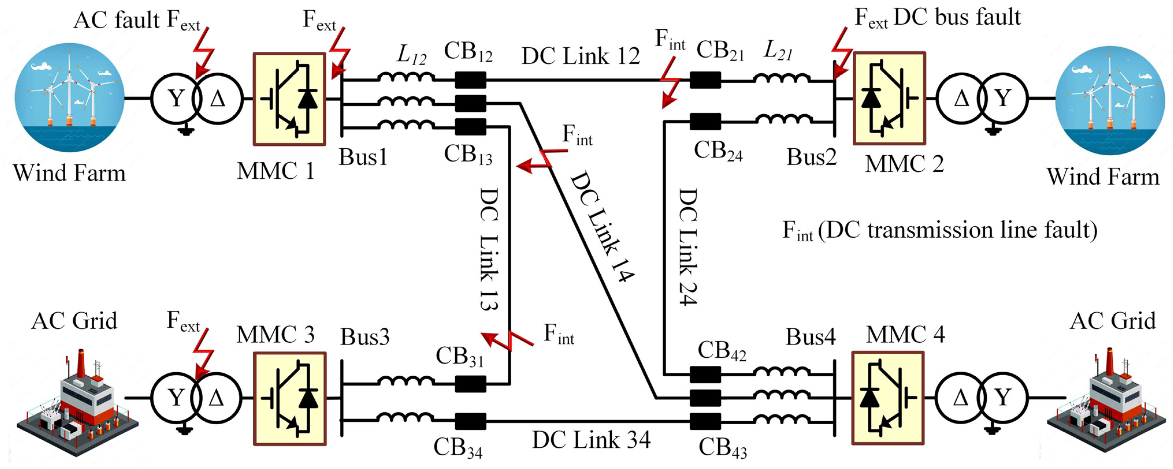
The proposed system model is based on the MT-HVDC grid using PSCAD / EMTDC software, whereas its features are presented in [32]. As shown in Figure 1, two offshore wind farms (Converter 1 and 2) were connected to two onshore converters (Converter 3 and 4) that transmit electrical power to the mainland AC grid. The configuration for onshore and offshore converters is a half-bridge modular multilevel converter (MMC). The rated power for MMC 1,2, and 3 was 900 MVA, whereas MMC 4 rated power was 1200 MVA. The undersea cable system connected these converters via five DC links. There was a symmetric monopole configuration with a DC link voltage of ±320 kV. The two DC links (i.e., 13 and 14) had a 200 km length, one DC link (i.e., 24) had a 150 km length, and two DC links of 100 km (i.e., 12 and 34).

The hybrid HVDC circuit breaker (DCCB) had a fast-operating time of 1–2 ms and utilized 100 mH inductors (L) at each link border to form a reliable electrical connection. The protection system used full-selective fault-clearing to ensure stability and minimize the impact of faults on the overall system. In this strategy, each link was treated as an independent protection zone and was only de-energized during a fault condition while the remaining grid remained up and running. This approach reduced the disruption caused by faults and helped maintain the system’s stability. Note that F_int refers to a failure that occurred within the DC transmission lines, and F_ext stands for AC and DC bus faults.

2.2. Fault Analysis

An intelligent plan for protecting DC transmission lines consists of two fundamental elements: input feature vectors and learning models. Input feature vectors are a set of variables or parameters used to describe the system’s current state and are used as input to a learning model. These feature vectors can include information such as current and voltage values that can provide insight into the condition of the HVDC system. Therefore, we introduce a fault analysis section for the current and voltage values.

During a DC fault, the current in the HVDC grid will increase rapidly, and the voltage will drop sharply. This is because the fault causes a short circuit, which increases the current flowing through the system, and the voltage drop is a result of the increased current flowing through the resistance of the system. In summary, V_F and I_F are used to distinguish between external (F_ext) and internal (F_int) faults in a VSC-based MT-HVDC configuration. The classification of external solid faults and high-resistance internal faults is particularly difficult. To simplify the analysis, only internal faults (F_int) were considered. The DC line voltage at the fault location was abruptly reduced to zero when there was a fault. The change in voltage is mathematically expressed as follows [6]:

$$V_{F_{int}}=\frac{Z_{impedance}/2}{{(R}_f+\raisebox{1ex}{$Z_{impedance}$}\!\left/ \!\raisebox{-1ex}{$2$}\right.)}(-V_{DC0})$$

(1)

Equation (1) reveals that the voltage change was divided over the cable and the fault resistance (R_f). As the factor (1/2) indicates, the cable impedance (Z_impedance) was in series with the fault resistance. A similar relationship can also be found in DC line voltage with an external fault [23]:

$$V_{F_{Ext}}=\frac{Z_{impedance}}{(sL+Z_{impedance})}(-V_{DC0})$$

(2)

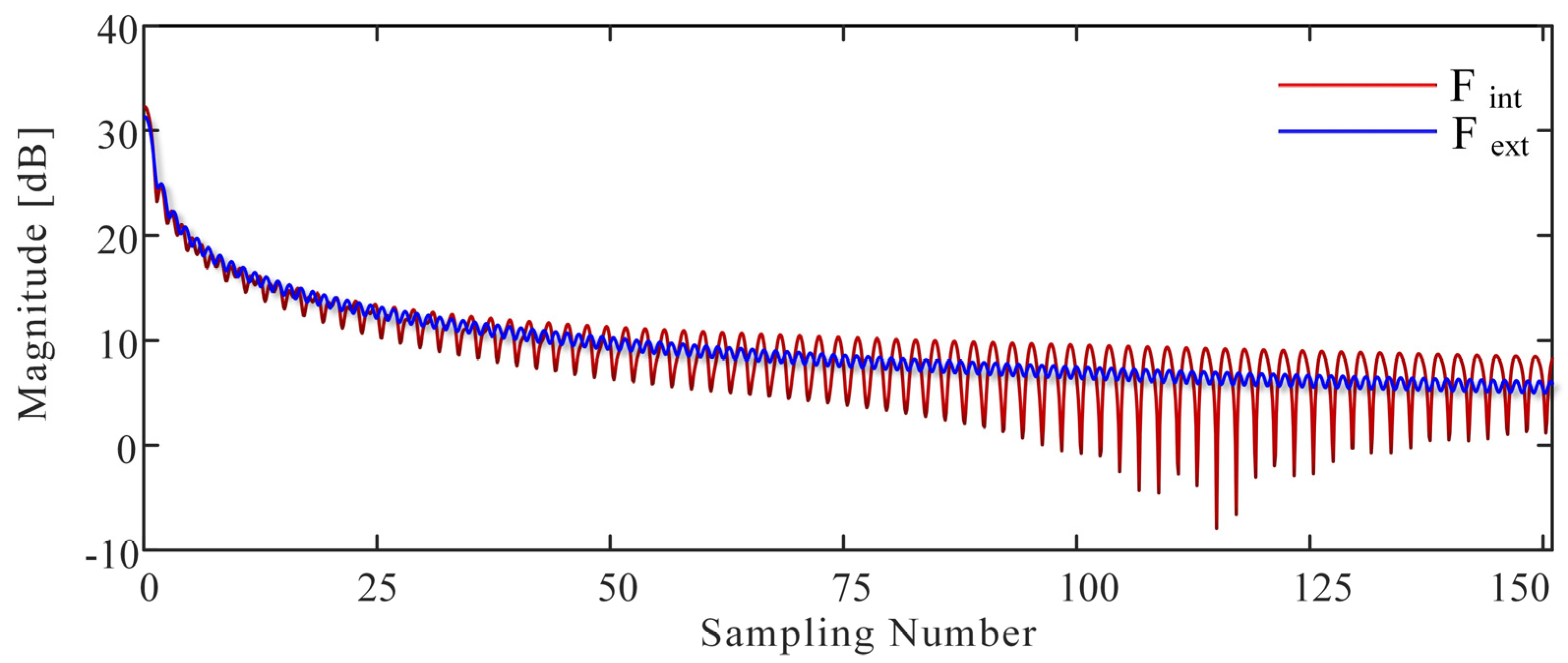
Based on Equation (2), voltage was divided between the cable and inductor (sL). The difference between equations 1 and 2 is the presence of an inductor. The presence of the inductor L caused the circuit to have poles. High frequencies were filtered out by a series inductor during F_ext, while fault voltages were dampened by fault resistance during F_int. Figure 2 illustrates the graphical representation. An internal fault created a steeper DC line voltage curve compared with an external fault. Figure 3 provides evidence of the low-pass filtering effect of inductor L during an external fault. This component effectively allowed low-frequency components to pass through while filtering out high-frequency components, providing a more stable and controlled response to external faults.

Similarly to DC line voltage, DC line current can also contain high-frequency components under internal faults DC inductor inherent boundary, and the location of the fault can also affect the frequency of these components. This information can be used to identify the location and type of internal fault. This work has studied two internal fault types: pole-to-pole (PTP) and pole-to-ground (PTG). DC bus and AC faults have been considered external faults.

The SWT was utilized to extract fault signal features, and the Daubechies mother wavelet was explicitly chosen for its resemblance to the signal being analyzed. It was used in the proposed fault diagnostic scheme for identifying internal and external faults by analyzing the high-frequency component of the DC line voltage and the DC line current characteristics in the frequency domain.

3. Stages of the Proposed Algorithm

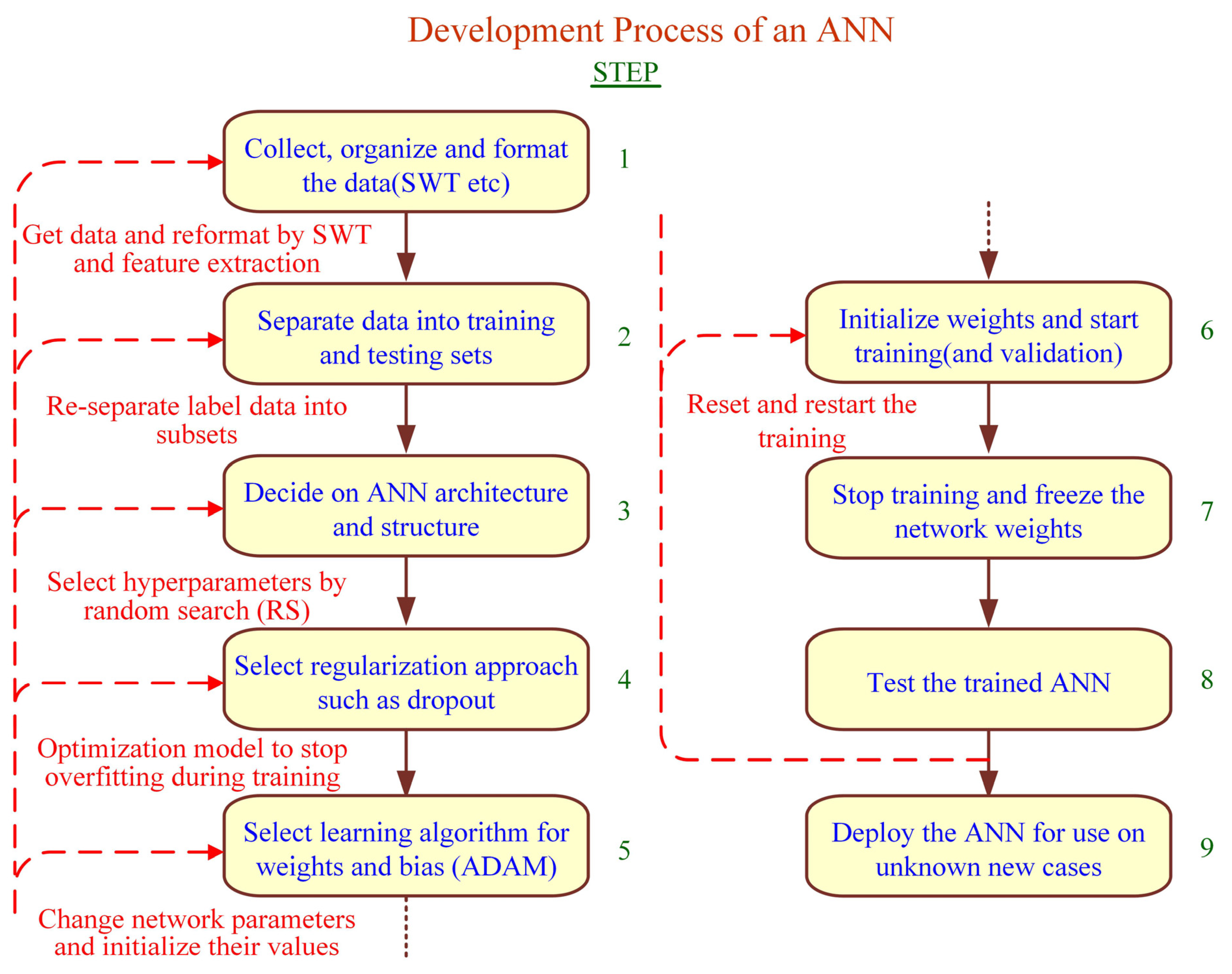
Figure 4 describes the five main stages of the proposed RS-based ANN. In step 1, the intelligent algorithm samples the relevant values for a 3-ms time window. With the use of SWT, distinctive characteristics of transient fault currents and voltages were collected. It should be noted that each sample contained voltage and current information in time and frequency. To detect and discriminate faults, these features were further scaled down to reflect the status of the MT-HVDC in replicated transient occurrences in step 3. In step 4, RS was applied to optimize the hyperparameters of the ANN model and use the mean square error as a metric to select the most appropriate model. Finally, a trained ANN model was used to detect new faults.

3.1. Step 1—Signal Acquisition

First, DC transmission line voltage and current signals were captured from positive and negative poles at high sampling rates of 50 kHz after analyzing the fault. The samples were then filtered to remove aliasing artifacts and divided into three-ms time windows for processing by the Stationary Wavelet Transform filters. We generated samples for training based on variations in fault distance and resistance.

Table 1. Case studies for internal faults in training data.

Time Window Span [0–0.8, 0.8–1.5, 1.5–3.0 ms]	Samples Quantity	Fault Resistance (Ω)	Fault Remoteness (km)	Noise (dB)
1st Segment	189	0.01, 25, 50, …, 175, 200	1, 10, 20, …, 180, 190, 198	20, 25, 30
2nd Segment	273	0.01, 25, 50, …, 275, 300	1, 10, 20, …, 180, 190, 198	20, 25, 30
3rd Segment	357	0.01, 25, 50, …, 375, 400	1, 10, 20, …, 180, 190, 198	20, 25, 30

A total of 819 faulty samples for each fault type (i.e., PTP and PTG), Making a total of [(F_int = 819 × 2)] = 1638 internal training samples. Data have been extracted from DC links 12, 13, and 14 for internal faults.

and

Table 2. Case studies for external faults in training data.

Variable	Details
Fault type	Single and Multiple AC type faults
Fault Resistance (Ω)	0.01, 50, 100, 150, 200
Noise (dB)	20, 25, 30

Total AC faulty sample = 165, Total DC-bus faulty sample = 36 (Fault Resistance from 5–115 Ω and 10 Ω step size) have been collected around MMC 1, 2, and 3. Total training samples = G = [(F_total = (1638 + 201))] = 1839.

illustrates fault scenarios. There were 819 PTP and 819 PTG fault samples, whereas the total internal fault samples were 1638. We had 165 AC faulty samples for external fault cases and 36 DC bus faulty samples. This step is essential because it allows the algorithm to extract relevant information from the signals that can be used to detect and discriminate faults in the MT-HVDC system. Furthermore, when an internal fault occurs in the DC line, the criteria $(d{V}_{DC}/dT)$ are activated, which can also be used as a start-up element.

3.2. Step 2—Stationary Wavelet Transform

Because the wavelet transform can analyze signals simultaneously in both the frequency and time domains, as a powerful tool, it ensures the safety of the power system. By doing so, it can detect singularities in signals caused by unwanted events in the power system and extract useful data from measured quantities. CWTs (continuous wavelet transforms) and DWTs (discrete wavelet transforms) are two kinds of wavelet transforms. Processor requirements and the desired level of time resolution determine the choice between CWT and DWT.

The DWT is a popular method in MT-HVDC protection due to its computational efficiency and simplicity. However, one of the main drawbacks of DWT is the loss of high-frequency information content caused by the down-sampling process at each decomposition level. The Stationary Wavelet Transform (SWT) is often used to overcome this limitation. Unlike DWT, SWT does not down-sample the analyzed signal. Instead, it uses high-pass and low-pass filters to up-sample by a factor of two at every level of decomposition through zero padding, preserving high-frequency information content.

The stationary wavelet transform preserves the original time information of the analyzed signal. This is because it results in an output with the same number of coefficients at every level of decomposition. Unlike the DWT, the SWT algorithm achieves this by applying discrete convolution to the signal using appropriate low-pass and high-pass filters without the need for down-sampling. Note that SWT’s output is redundant; hence, it requires more storage space than DWT. However, the time and frequency information are preserved. 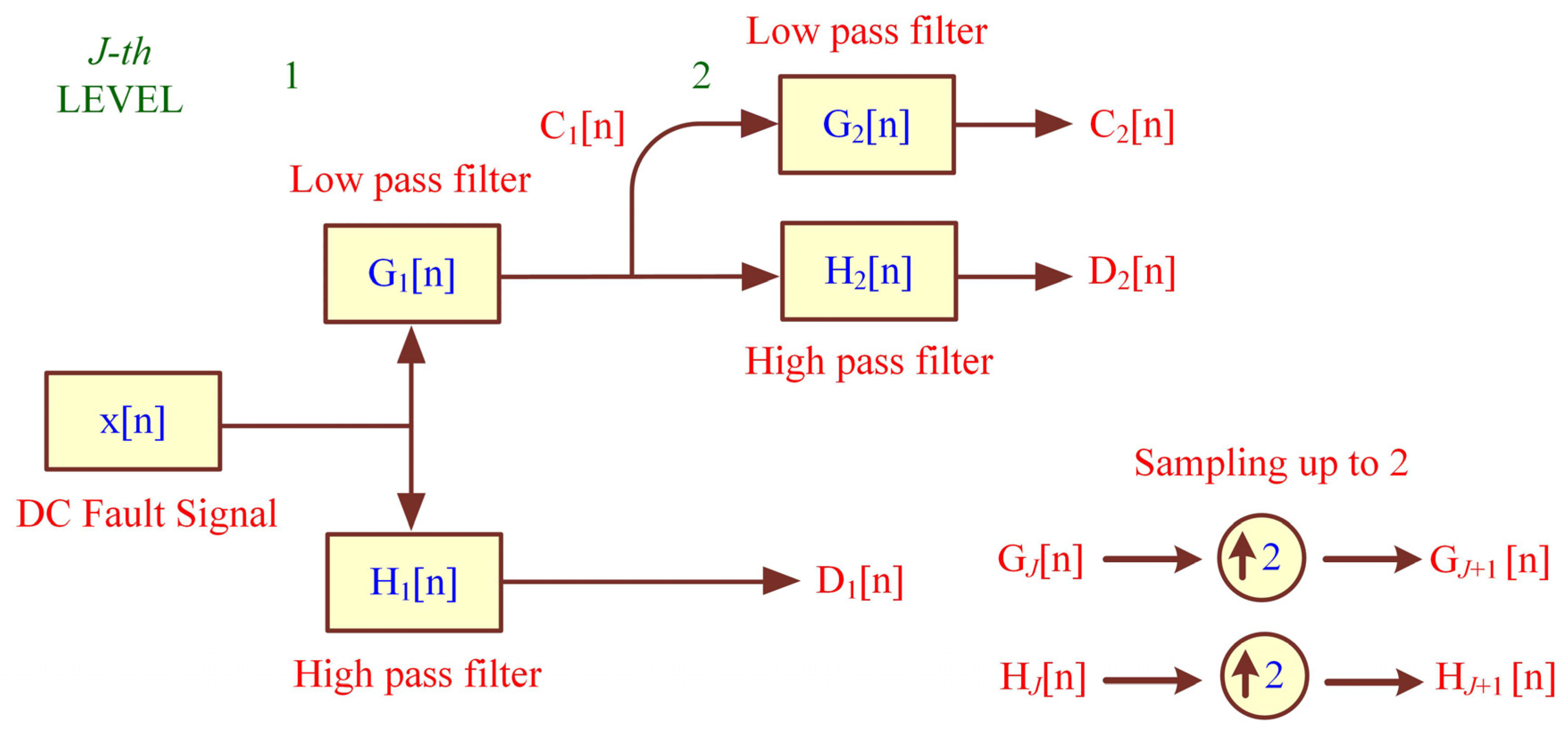Figure 5 displays the SWT procedure up to the second level of decomposition.

The SWT provides a multi-resolution representation of the signal, allowing for better analysis and detection of specific features in the signal, such as DC faults. While decomposing DC fault signals x[n], ${\mathrm{H}}_J\left[\mathrm{n}\right]$ high pass and low pass filters ${\mathrm{G}}_J\left[\mathrm{n}\right]$ were used at J-th level, ${\mathrm{C}}_J\left[\mathrm{n}\right]$ and ${\mathrm{D}}_J\left[\mathrm{n}\right]$ represent approximation and detail coefficients at J-th level. A high pass ${\mathrm{H}}_J\left[\mathrm{n}\right]$ and low pass ${\mathrm{G}}_J\left[\mathrm{n}\right]$ filter was obtained by up-sampling the filters from the previous level ($J-1$) and convolving them with the approximation coefficient at that level ($J-1$) to extract decomposition at level $J$. At this level, you will be able to obtain detail and approximation coefficients. Decomposition was performed iteratively until the desired number of levels is reached. A detailed coefficient for each level of decomposition $J$ was calculated using (3).

$${\mathrm{D}}_J\left[\mathrm{n}\right]=\sum _{m=0}^{M-1}{\mathrm{C}}_{J-1}\left[k\right]\times {\mathrm{H}}_J[\mathrm{n}-k]$$

(3)

In this Equation, $k$ represents the sample index and $M$ is the order of the high-pass filter ${\mathrm{H}}_J\left[\mathrm{n}\right]$. The desired number of decomposition levels is 1 and 2 in this proposed approach. Decomposition at level 1 yielded a coarse representation of the signal, while decomposition at level 2 yielded a detailed presentation.

The dB-4 wavelet is a member of the Daubechies wavelet family and was selected in this particular study. It is well-suited for signal processing applications that require both time and frequency resolution. This is why it is often used in image compression, signal denoising, and feature extraction.

3.3. Step 3—Feature Extraction

This process involved extracting features from three transient periods of 0–0.8 ms, 0.8–1.5 ms, and 1.5–3.0 ms by monitoring certain parameters. The Stationary Wavelet Transform (SWT) was then applied to each period to obtain detail coefficients at the first and second levels. The required number of samples for each transient period was eight. The numerical values obtained from each transient period were used to calculate various feature vectors. These feature vectors included:

• Energy content: $E\left(D_J\right)$, which represents the amount of energy present in the detail coefficients.
• Mean: $\mathrm{\mu }\left(D_J\right)$, which represents the average value of the detail coefficients.
• Standard deviation: $\sigma \left(D_J\right),$ representing the degree of variation or dispersion of the detail coefficients.
• Sum: $\sum {(D}_J),$ which represents the total value of the detail coefficients.

These feature vectors were calculated using mathematical equations that involve the detail coefficients $D_J$ obtained from the SWT. The mathematical Equation for each feature is presented as follows:

$$\sum (D_J)=\sum _{n=1}^{k_w}\left|D_J\left(n\right)\right|$$

(4)

$$\mathsf{\mu }\left(D_J\right)=\frac{1}{2^J\times k_w}\sum _{n=1}^{k_w}\left|D_J\left(k\right)\right|$$

(5)

$$\sigma {(D}_J)=\sqrt{\frac{1}{2^J\times k_J}\sum _{k=1}^{k_w}{\left(\right|D_J\left(n\right)|-\mathsf{\mu }(D_J\left)\right)}^2}$$

(6)

$$E\left(D_J\right)=\sum _{n=1}^{k_w}{\left[D_J\left(n\right)\right]}^2$$

(7)

$D_J\left(n\right)$ is the n-th detail coefficient for each decomposition level $J$ = 1, 2 and $k_w$ indicates the size of the window. Normalizing the feature vectors is a common preprocessing step in machine learning. This can be achieved by removing the mean of the data set and dividing it by the standard deviation, resulting in a scaled version with zero mean and a standard deviation of one. This can help improve the performance of some machine learning models by ensuring that the features are on a similar scale and that outliers do not unduly influence the model. Mathematically represented as:

$${p\left(i\right)}_{scalling}=\frac{p\left(i\right)-\overline{P}}{\sigma \left(P\right)}$$

(8)

Typical values for $p\left(i\right)$ represent the i-th sample in the feature set $“p”$, the mean of the selected feature calculated from the training set is denoted as $\overline{P}$ and the standard deviation of each feature is represented by $\sigma \left(P\right)$.

3.4. Step 4—Network Optimization

In this section, ANN, architecture layout, hyperparameters, and ANN optimization have been presented.

3.4.1. Artificial Neural Network (ANN)

ANNs aim to learn patterns from data through training, an approach inspired by the human brain. ANNs are composed of hundreds of individual units called neurons connected by weights and organized into layers. They consist of a typical input layer, an output layer, and a hidden layer. Neurons receive input data in the input layer, and the output layer produces the desired response. A neural network can understand inputs correctly because of the structure of its layers and connections. During training, each neuron is activated by the weighted sum of its inputs, and a transfer function is used to generate output. This transfer function adds nonlinearity to the network during training. As the network is trained, the connections between neurons are optimized until the prediction error is reduced and a particular level of accuracy is reached. With the right training and testing, a network will be able to make predictions about new inputs.

3.4.2. Architecture Layout

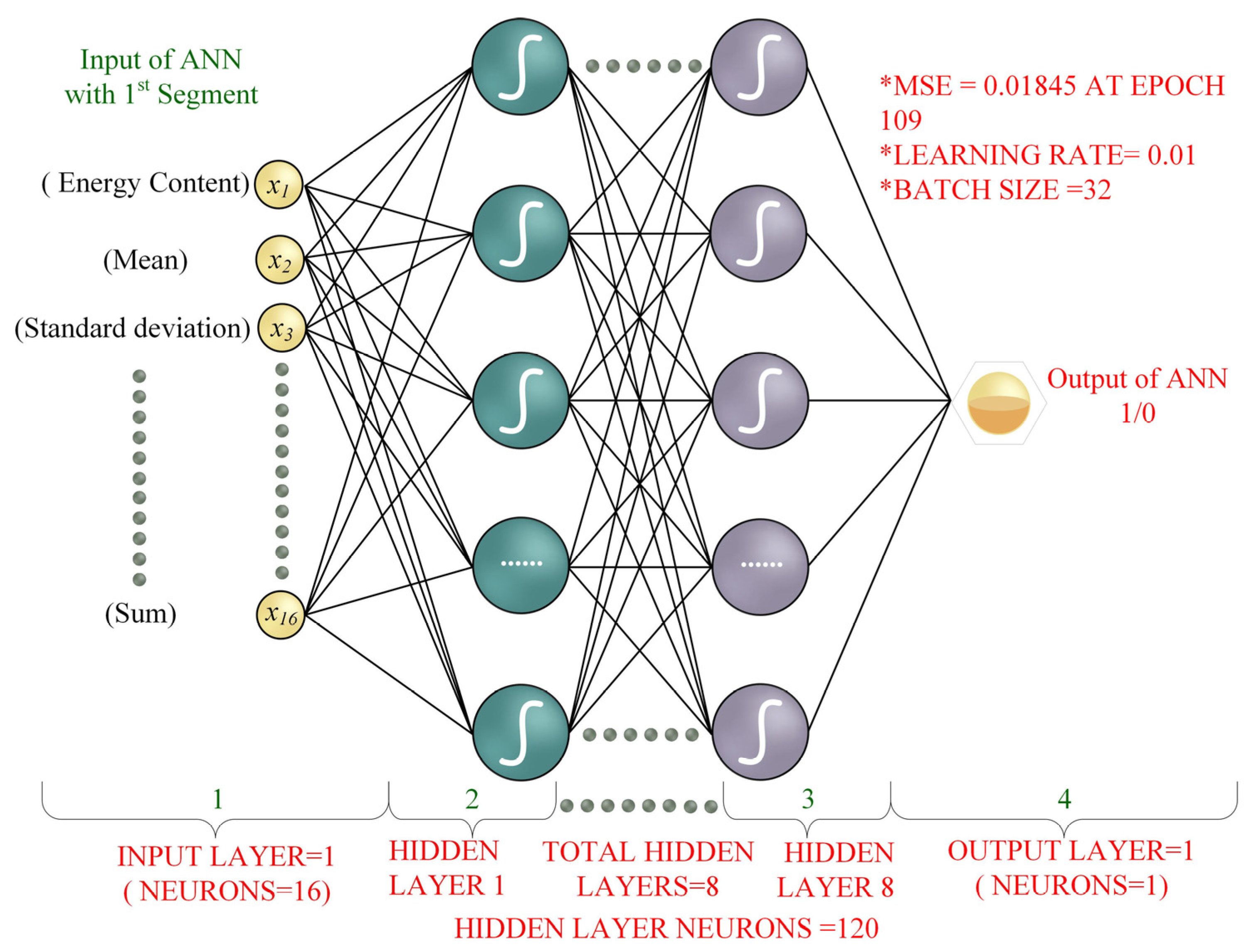
Four vectors represent a DC line fault for each transient period (0–0.8 ms, 0.8–1.5 ms, and 1.5–3.0 ms). The first two vectors contain information about DC fault current from positive and negative poles, while the next two are related to DC fault voltage from positive and negative poles. Energy content, mean, sum, and standard deviation represent each power signal’s information. The general design is given in Figure 6.

Representing the input vector for the first segment as X = (x₁, x₂, x₃, x₄, …, x₁₆)^T, the output vector as O = (o₁)^T, and the hidden layer output as H = (h₁, h₂, h₃, …, h_t)^T, the signal generation of ANN for a first segment can be indicated as:

$$h_q=f\left(\sum _{r=1}^{16}{w}_{r,q}\times x_r+b_q\right), q=1, 2, 3, 4, \dots , t$$

(9)

$$O_s=f\left(\sum _{q=1}^t{w}_{q,s}{h}_q+b_s\right), s=1$$

(10)

The weights and biases in an artificial neural network determine how the input is transformed into output. $w_{(r,q)}$ and $b_q$ are the weights and biases determining the transformation of the input to the subsequent layer (i.e., hidden layer) in Equation (9). In Equation (10), $w_{(q,s)}$ and $b_s$ denote the weight and bias from the hidden to the output layer. Training error can be reduced by using an activation function, abbreviated as f.

3.4.3. Hyperparameters

Weights and biases are parameters of a model that are managed to learn throughout the training process. In contrast, hyperparameters are parameters that are established beforehand in the training process. Optimizing the hyperparameters in a neural network is an important step in achieving good performance, as they directly affect the training process and the strong generalization abilities of ANNs. Hyperparameter optimization involves combinatorial optimization, which is very challenging and time-consuming.

3.4.4. Random Search

Random search optimization is a simple yet effective method for tuning the hyperparameters of an artificial neural network. One advantage of random search is that there is no dependency on any gradient information, and it can be applied to many neural network architectures. Additionally, it is relatively computationally inexpensive and can be helpful in quickly identifying a good set of hyperparameters for further fine-tuning with more sophisticated optimization methods.

The idea behind this method is to randomly generate a set of hyperparameters and evaluate their performance on the training dataset. The study used k-fold cross-validation to evaluate the ANN model’s performance [33]. The evaluation metric used was the mean squared error (MSE). It is represented as follows:

$$MSE=\frac{{\sum }_{i=1}^l\left|{(y_l-x_l)}^2\right|}{l}$$

(11)

The predicted value is $y_l$, and the true value is $x_l$, where $l$ denotes the sample size and k = 5 in this work. Hyperparameters being searched in this case include the number of hidden layers, the batch size, the learning rate, and the number of neurons per hidden layer. The most accurate ANN classifier is the model trained using the optimum set of hyperparameters. The ideal number of neurons is 8 for hidden layers, and the learning rate is 0.01. The MSE is 0.0124 with 100% training accuracy. Figure 7 shows the RS results.

Apart from the hyperparameters mentioned above, the other parameters were adjusted in accordance with the Matlab framework. To enhance the performance of the ANN classifier and reduce overfitting to the training data, a drop-out strategy was implemented to limit interdependent learning among the hidden layer neurons during the training phase. Adam optimization was also used for optimization, and one neuron performs a binary classifier at the output layer. Due to the log-sigmoid functions used as activation functions in the output layer of the ANN model, the output varies from 0 to 1. In this study, a decision threshold of 0.9 was chosen to translate the predicted probability rate into a class label (0 or 1) based on the log-sigmoid function during the training and testing phases. Therefore, output 1 represents an internal failure that results in a trip signal when the probability is higher than 0.9. The overall development of ANN and its optimization is shown in Figure 8.

3.5. Step 5—Binary Classifier with Multiple Segments

A normalized input vector will be input into a neural net classifier. The classifier will output a binary signal to distinguish between internal and external disturbances. An output of 1 indicates an internal fault, which activates the circuit breaker to protect the DC transmission lines. An output of 0 indicates an external fault or disturbance.

4. ANN with Multiple Segments

There is considerable evidence that ANNs can help diagnose faults quickly and accurately in power systems [34,35,36]. The input vectors for three segments are used to train artificial neural networks with different objectives in the presented work. It is mentioned in the next section in detail. The first segment is designed to detect DC line faults with fast response, the second segment is to nullify the effect of relay failure with minimal disturbance to the grid, and the third segment is implemented to detect high impedance faults as DC fault current becomes less prominent in these cases.

A high-impedance fault in a power system can be located efficiently and effectively by this technique while reducing the computational burden. The low transient fault current of high-impedance faults makes them challenging to identify, but this method addresses this using different relay segments. When the fault resistance is small, the algorithm uses a small-time window and the first segment of the relay, resulting in a fast response. In cases where 1st segment fails, or the fault impedance is high, the algorithm shifts to the second or third segment. While the segment adds delay to the response, these are manageable due to low fault currents at high impedances. This approach allows for a more efficient and reliable way of detecting and responding to high-impedance faults without the need for additional backup protection. The proposed relay can itself detect and deal with the failure.

Relay Design

The strategy for the relay design is shown in Figure 9. Once the $({dV}_{DC}/dT)$ criteria is activated, and analogue signals are gathered by current and voltage transducers (CT & VT) with a sampling circuit and converted to digital by an analogue-to-digital (A/D) converter. Using real-time SWT, an A/D converter extracted spectral features from the sampled signal spanning 0–0.8 ms, 0.8–1.5 ms, and 1.5–3.0 ms. These features were used as input for an ANN. 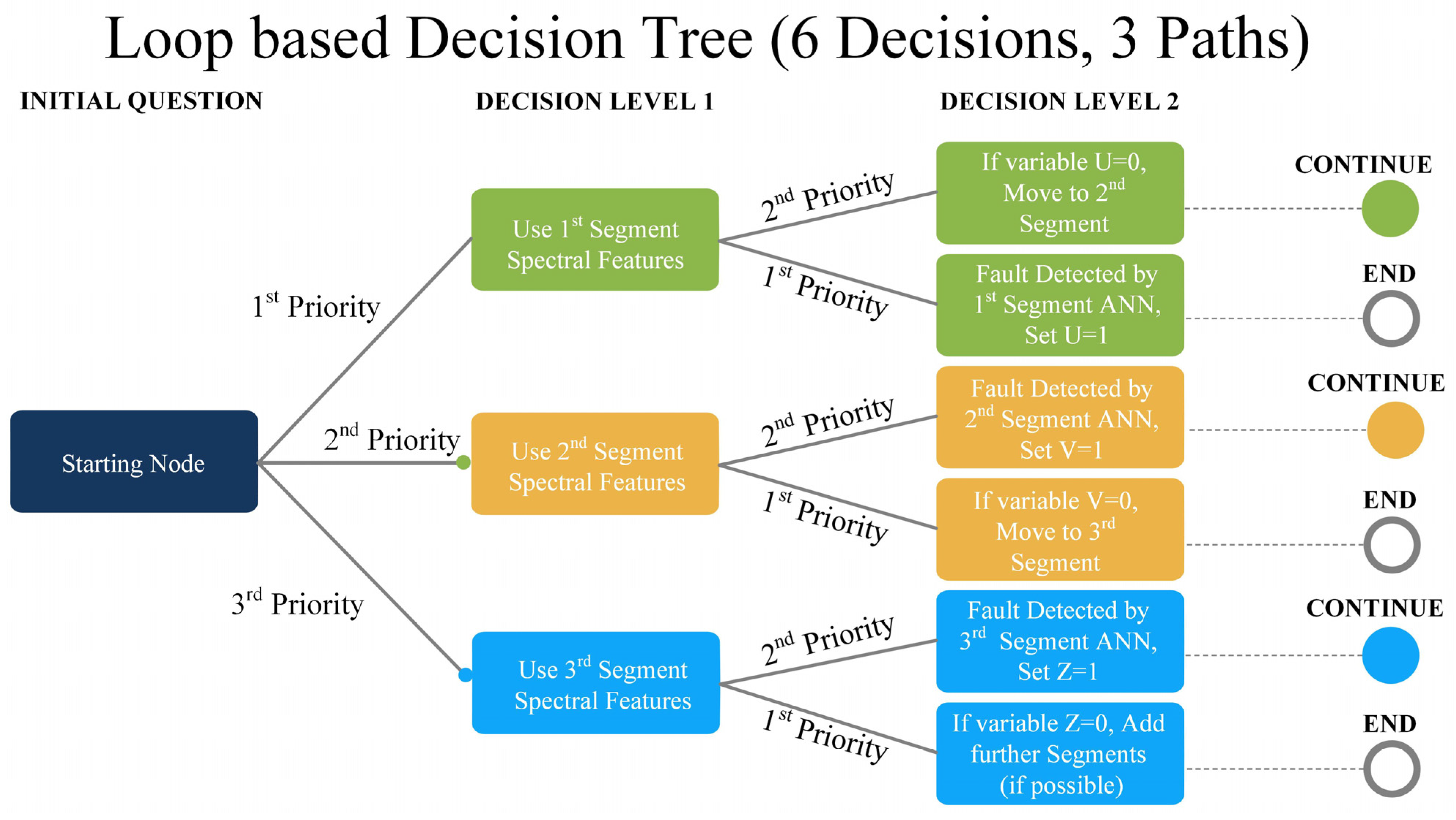Figure 10 shows how a loop-based decision tree was used to implement relay logic and operate the circuit breaker using the output from the well-trained and optimized ANN.

This decision tree has three levels of decision-making, with the first level having three priority lists. The use of priority lists at the first level ensures that the most critical issues are addressed first. At the second level, there are two priorities, and different actions will be taken depending on whether a fault is detected or not. If a fault is detected, set variable U to 1 and send a trip signal to shut down the system. If a fault is not detected at the first segment, move to the second priority of the decision level one. Then, the 2nd segment-based ANN input will be added to the 1st segment ANN to send a trip signal. If still no fault is detected, variable V will be set to 0, and the 3rd segment ANN will be used to make a final decision. Overall, this decision tree is well-designed to effectively and efficiently handle any potential issues that may arise.

5. Time Delays Anticipated for the Proposed Scheme

For a time-domain method to be successful in real-life implementation, it must be tested in a realistic environment that includes expected delays. An operating time measurement can be performed by considering the delays associated with window-based processing $t_{\mathrm{t}\mathrm{i}\mathrm{m}\mathrm{e}-\mathrm{w}\mathrm{i}\mathrm{n}\mathrm{d}\mathrm{o}\mathrm{w}}$, data processing $t_{\mathrm{d}\mathrm{a}\mathrm{t}\mathrm{a}-\mathrm{p}\mathrm{r}\mathrm{o}\mathrm{c}\mathrm{e}\mathrm{s}\mathrm{s}\mathrm{i}\mathrm{n}\mathrm{g}}$ and the time $t_{binary-decision}$ needed to produce a binary decision by the ANN. The following is the numerical representation:

$$T_{Total}=t_{\mathrm{t}\mathrm{i}\mathrm{m}\mathrm{e}-\mathrm{w}\mathrm{i}\mathrm{n}\mathrm{d}\mathrm{o}\mathrm{w}}+t_{\mathrm{d}\mathrm{a}\mathrm{t}\mathrm{a}-\mathrm{p}\mathrm{r}\mathrm{o}\mathrm{c}\mathrm{e}\mathrm{s}\mathrm{s}\mathrm{i}\mathrm{n}\mathrm{g}}+t_{binary-decision}$$

(12)

In this case study, $t_{\mathrm{t}\mathrm{i}\mathrm{m}\mathrm{e}-\mathrm{w}\mathrm{i}\mathrm{n}\mathrm{d}\mathrm{o}\mathrm{w}}$ depended upon the window length for processing the feature vectors and sampling time. Taking the 50 kHz sampling frequency into account, $t_{\mathrm{t}\mathrm{i}\mathrm{m}\mathrm{e}-\mathrm{w}\mathrm{i}\mathrm{n}\mathrm{d}\mathrm{o}\mathrm{w}}$ for the first segment was equal to 0.8 ms + 20 µs. For the second segment, $t_{\mathrm{t}\mathrm{i}\mathrm{m}\mathrm{e}-\mathrm{w}\mathrm{i}\mathrm{n}\mathrm{d}\mathrm{o}\mathrm{w}}$ = 1.5 ms + 20 µs, and $t_{\mathrm{t}\mathrm{i}\mathrm{m}\mathrm{e}-\mathrm{w}\mathrm{i}\mathrm{n}\mathrm{d}\mathrm{o}\mathrm{w}}$ = 3 ms + 20 µs for the third segment.

The personal computer took around 50–100 µs for data processing ${(t}_{\mathrm{d}\mathrm{a}\mathrm{t}\mathrm{a}-\mathrm{p}\mathrm{r}\mathrm{o}\mathrm{c}\mathrm{e}\mathrm{s}\mathrm{s}\mathrm{i}\mathrm{n}\mathrm{g}})$. However, a 0.5–1 ms delay can be added to the impersonator to compute practical protection devices [21]. Several factors influence the time it takes for the ANN to generate tripping signals, such as the algorithm’s complexity, the code’s efficiency, and the system’s power. The only way to evaluate $t_{binary-decision}$ is through experimentation, which we consider for future work.

6. Results and Discussions

It involves training an ANN with pre-existing data during the offline training phase, followed by online fault detection. To evaluate the performance of the proposed scheme, fault scenarios (PTP and PTG), which have not been included in the training data, were introduced after the ANN has been trained. Using a metric known as the accuracy ratio, we assessed the accuracy of a model:

$$Accuracy metric=\left(1-\frac{{AM}_e}{AM}\right)100\%$$

(13)

The value of AM represents the size of the dataset used for testing, while AM_e represents the number of incorrect classifications made by the model on the testing sets.

Table 3. Case studies for internal faults in testing data.

Time Window Span [0–0.8, 0.8–1.5, 1.5–3.0 ms]	Samples Quantity	Fault Resistance (Ω)	Fault Remoteness (km)	Noise (dB)
1st Segment	160	10, 35, 60, …, 160, 185	5, 15, 25, …, 175, 185, 195	20, 25, 30
2nd Segment	240	10, 35, 60, …, 260, 285,	5, 15, 25, …, 175, 185, 195	20, 25, 30
3rd Segment	320	10, 35, 60, …, 460, 485	5, 15, 25, …, 175, 185, 195	20, 25, 45

A total of 720 faulty samples for each fault type (i.e., PTP and PTG), Making a total of [(F_int = 720 × 2)] = 1440 internal testing samples. Data has been extracted from DC links 12,13 and 14 for internal faults.

and

Table 4. Case studies for external faults in testing data.

Variable	Details
Fault type	Single and Multiple AC type faults
Fault Resistance (Ω)	0.1, 25, 75, 125, 175

Total AC faulty sample = 165, Total DC faulty sample = 33 (Fault Resistance from 10–110 Ω and 10 Ω step size) have been collected around MMC 1, 2 and 3. Total testing samples = G = [(F_total = (1440 + 198))] = 1638.

present the parameters of the newly introduced test fault cases. There are 720 PTP and 720 PTG fault samples, whereas the total internal fault samples are 1440. We have 165 AC faulty samples for external fault cases and 33 DC bus faulty samples.

6.1. Case Study 1 (Testing Scenarios)

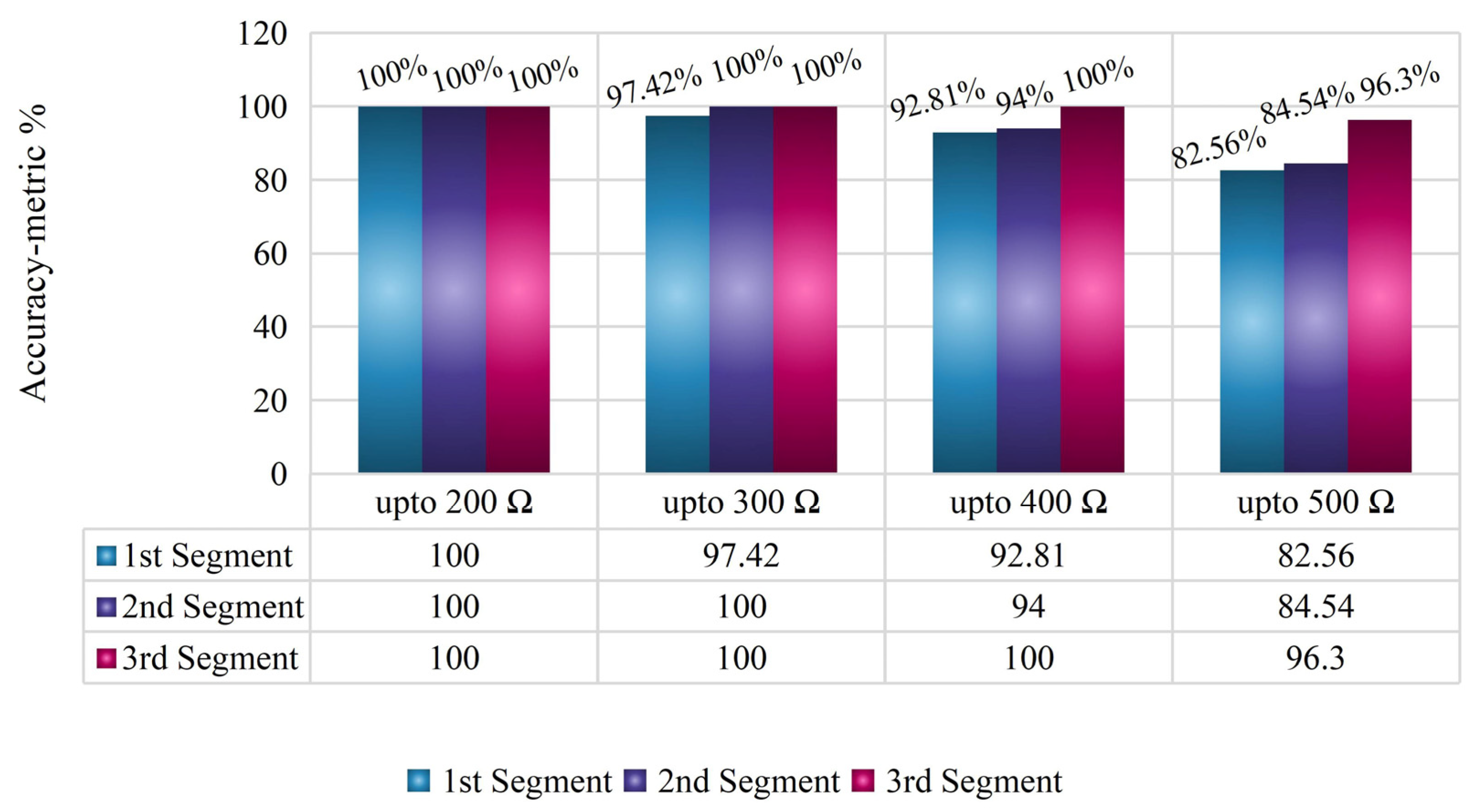
The proposed algorithm’s results on new testing samples are shown in Figure 11. It can be observed from Figure 11 illustrates that the relay was able to accurately detect all faults till the fault impedance of 400 Ω. If the fault impedance was less than 200 Ω on the DC line, the design relay’s first segment could detect it with minimal detection delay. The detection delay was minimal, even if the fault occurred at the farthest end of the DC line. It was, however, slightly less likely for the first segment to identify faults when the fault impedance exceeds 200 Ω (i.e., between 200 Ω and 300 Ω, it goes to 97.42%). The average fault detection ability for 1st segment was 93.20% (i.e., between 10 Ω to 500 Ω). The 2nd segment of the designed relay restored this failure with 100% accuracy between 200 Ω and 300 Ω. A high impedance fault caused less of an impact on the rising value of DC fault current in the second millisecond, mainly when it occurred at the farthest end. The second segment can detect faults up to 300 Ω impedance. Faults more significant than 300 Ω were detected in the third segment of the designed relay, as the third threshold could detect faults up to 400 Ω. The average fault detection ability for the 2nd segment was 94.64% (i.e., between 10 Ω to 500 Ω). Plus, all segments have been tested and found to be fully functional and did not respond to external faults without any errors and had 100% accuracy.

Above all, the arrival time of the travelling wave at a given fault location may fluctuate depending on the type of fault. As a result, different faults may be processed at different speeds. However, this delay was still minimal and acceptable for DC applications.

6.2. Case Study 2 (Noisy Events)

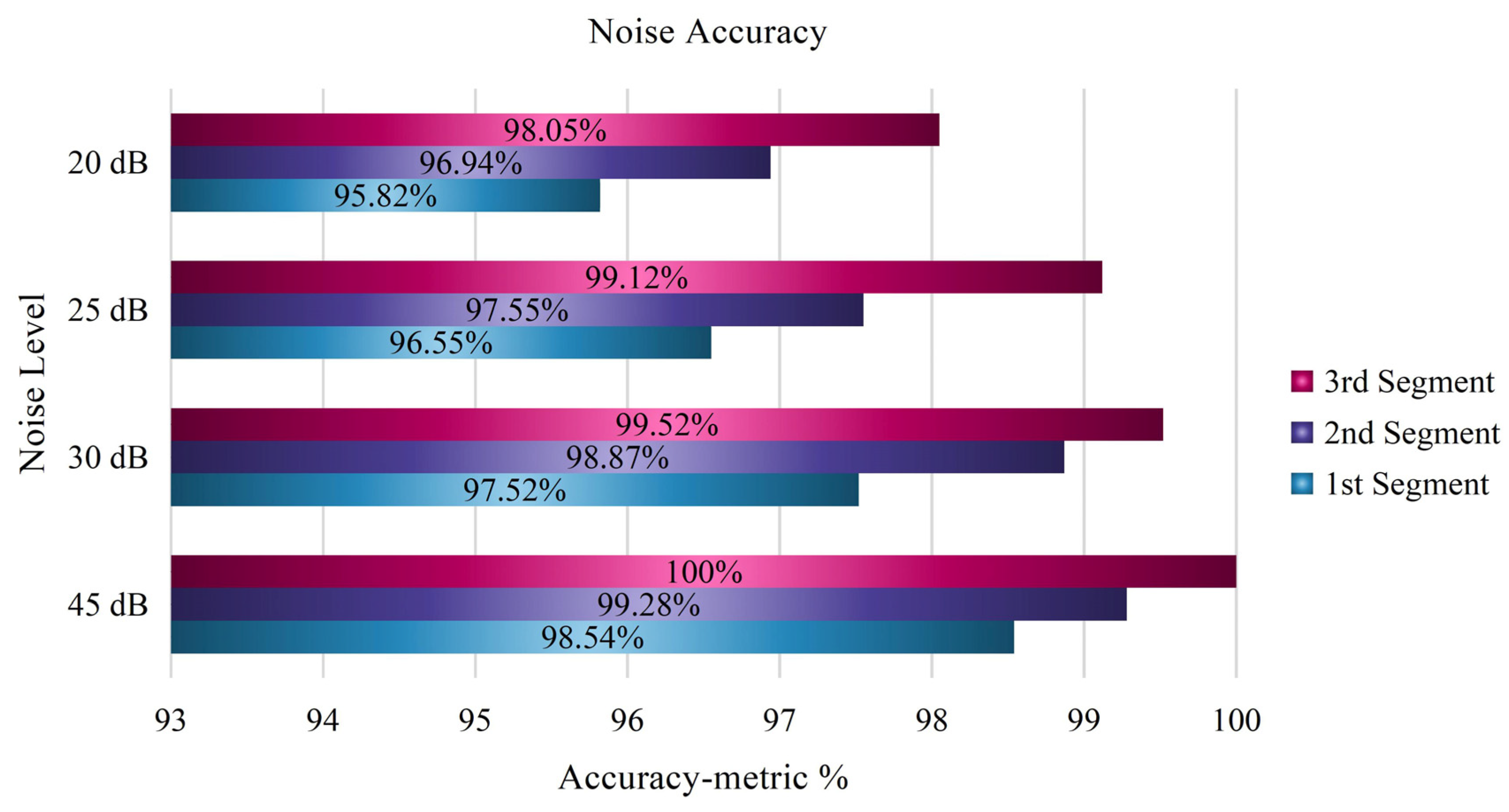
The proposed method for fault detection is robust and reliable, even in the presence of noise. The method can be evaluated for its ability to function effectively and accurately despite interference by adding white Gaussian noise to the input signal. As shown in Figure 12, the results demonstrate that the method is highly accurate in detecting faults, even at low noise levels. At 45 dB noise, the method has a total accuracy of 99.27% for DC line faults. Additionally, the method maintains high performance at even lower noise levels, with an overall accuracy of 96.94% for PTP and PTG faults at 20 dB noise.

For each segment of Table 3, the first segment was accurate between 20–45 dB noise levels with 97.12%. In the second segment, the accuracy was 98.16%, and 99.20% for 3rd segment was between 20–45 dB noise level. These results indicate that the proposed method is reliable and robust in detecting faults in real-world scenarios where noise is present.

Further demonstrating the efficiency of the suggested method compared to other methods, it was tested under the same noisy event as mentioned earlier. The average accuracy of each segment is presented in

Table 5. Comparative analysis under the different noisy event.

Average Segments Accuracy	Suggested Solution	Simple ANN	BPNN
	97.12%	96.25%	94.82%
	98.16%	97.13%	96.11%
	99.20%	98.54%	97.21%
Overall	98.20%	97.30%	96.04%

. Regarding manually configured simple ANN, the proposed algorithm was five times faster for NN optimization. The overall accuracy was also lower (i.e., 97.30%), with six hidden layers and 15 neurons in each hidden layer. Additionally, the results support the claim that the suggested method is more accurate and robust than BPNN.

6.3. Case Study 3 (Segment Testing)

To realistically test the proposed ANN-based multiple time window segment relay protection strategy, a hybrid (H)-DCCB model as proposed by [37] was utilized in the test system. The aim was to detect and isolate the fault within a few milliseconds of its inception to avoid system downtime. This was primarily achieved without any secondary or backup protection, utilizing only multiple time window segments depending upon the magnitude of the fault resistance.

In this regard, a total number of ten hybrid-DCCBs were inserted in the test system. The specifications of the H-DCCB were altered as per MTDC grid specifications. Additionally, the self-level tripping mechanism of the breaker, as discussed in [37], was deactivated to subject the breaker components, i.e., IGBT valves and metal oxide surge arrestor (MOSA), to maximum fault stress during the required time window.

A total of three PTP fault case scenarios were simulated at a distance of 110 km from MMC-1 on DC-link 14. The fault resistance was adjusted following the segment of the time window under test, i.e., 35 Ω for 0.8 ms, 110 Ω for 1.5 ms, and 210 Ω for 3 ms.

6.3.1. Segment 1

The pre-fault current passing through the breaker was around 2 kA, and a 35 Ω low impedance fault was induced at t = 1.5 s for the first scenario. A rise in DC fault current and a steep decrease in the DC-link voltage was observed, as depicted in Figure 13a,b. The 0.8 ms time segment of the relay unit successfully identified a rapid increase in fault current. It took around 0.9 ms, including the 75 µs data-processing and 20 µs sampling frequency delay, to send a trip command. However, to mimic realistic conditions, the breaker was tripped after a further delay of approximately 0.1 ms due to internal delays associated with hybrid-DCCB, as shown in Figure 13e. Still, this limited the peak fault current to around 7 kA, significantly lower than the proposed 16 kA fault current interruption capacity outlined in [37]. Furthermore, the temperature and energy absorption stress in IGBT and MOSA, as illustrated in Figure 13c,d, were at nominal levels, as discussed in [37].

6.3.2. Segment 2

The second segment was designed to mitigate the effects of relay failure while causing little disruption to the grid. A moderate fault impedance value of 110 Ω was selected for the second scenario. As illustrated in Figure 14, a total of 1.6 ms relay delay and an additional 0.1 ms breaker delay was provided after the fault inception at t = 1.5 s. It can be seen that the breaker initiated the tripping sequence successfully at a DC fault current level of 3.3 kA. Furthermore, the temperature and energy stress was lower than that of the first scenario, as shown in Figure 14c,d.

6.3.3. Segment 3

Lastly, the third segment utilized a 3 ms time window and an additional 75 µs data-processing and 20 µs sampling frequency delay to send a trip signal to the breaker. This gave sufficient time to identify high-impedance faults since the DC fault current is less apparent in these instances. In addition, in a high impedance failure, a lower transient fault current peak is predicted; consequently, the relay unit must monitor the abnormal rise in fault current over a prolonged time frame so that IGBT valves are not thermally over-stressed. Figure 15c,d show that the breaker temperature and energy parameters were well below the maximum rated limits.

Hence, it is concluded that the relay protection scheme operates the breaker with minimal thermal and electrical stresses. Additionally, it provides a more efficient and reliable way of detecting and responding to high-impedance faults without the need for additional backup protection.

7. Comparison with Existing Methods

Compared to existing neural network-based protection algorithms [23,27,38], the proposed algorithm is more comprehensive and efficient. The use of direct faulty samples is further illustrated in [27], where a high workload is used to detect faults. It uses 13 ANN units for fault rectification. In [38], trip commands took around 4 ms, and the cases studied were not comprehensive. There was only an analysis of noise endurance up to 50 dB, whereas we studied fault cases up to 20 dB. In [39], a low number of fault cases were investigated, and noise endurance was not verified. Moreover, direct fault samples were integrated, which added extra computational burden. In [23], the fault recognition rate is low at high fault resistances (i.e., 84.5%) with no backup protection. The authors of [23] propose the use of another backup protection to cover main relay failures. However, the proposed strategy operates accurately even in high-fault resistance conditions (i.e., 96.30%), and multiple segments be used to cover failures.

Unlike [21,26], the proposed algorithm configures the ANN structure autonomously and does not require any new infrastructure or communication links. The proposed MMC-MTDC protection system is now more reliable and robust, overcoming the shortcomings of other solutions.

8. Conclusions

This scheme is able to detect and isolate faults more accurately by considering multiple segments of the transient period. This resulted in shortened fault detection times and increased DC grid reliability. Additionally, the ANN-driven approach makes the scheme more adaptable and able to handle more varied scenarios. Random Search enables the ANN to reach a level of performance that surpasses the traditional ANN learning model by optimizing hyperparameters. Aside from that, the model uses DWT-based robust features to capture the complex patterns of the fault current and achieve a high degree of accuracy in fault classification. The trained ANN can thus accurately and reliably detect faults in power system networks, regardless of the noise level. The comprehensive testing dataset is used to evaluate the proposed scheme’s performance in terms of accuracy and speed. Overall accuracy was 98.13% between 20 and 45 dB noise levels, and the minimum time to send a trip command was 0.9 ms. The results showed that the proposed scheme was able to accurately detect both internal and external faults with a high degree of reliability, robustness, and efficiency.

Control and protection are typically studied separately in the literature. However, optimal coordination between control and protection could ensure a reliable power supply. Therefore, future studies will investigate the coordination of protection and control.