Hybrid Vehicle CO₂ Emissions Reduction Strategy Based on Model Predictive Control

Abstract

This work proposes a hybrid drive controlled configuration, using a minimum emissions search algorithm, which ensures the operation of the Internal Combustion Engine (ICE) in its fuel efficiency range, minimizing CO${}_2$ emissions by controlling the power flow direction of the Electric Machine (EM). This action is achieved by means of Power Converters, in this case a bi-directional DC-DC Buck-Boost Converter in the DC-side and a DC-AC T-type Converter as the inverting stage. Power flow is controlled by means of a bi-directional Model Predictive Control (MPC) scheme, based on an emissions optimization algorithm. A novel drivetrain configuration is presented where both, the ICE and the EM are in tandem arrangement. The EM is driven depending on the traction requirements and the emissions of the ICE. The EM is capable of operates in motor and generator mode ensuring the Minimum Emission Operating Point (MEOP) of the ICE regardless of the mechanical demand at the drivetrain. Simulation and validation results using a Hardware in the Loop (HIL) virtual prototype under different operation conditions are presented in order to validate the proposed overall optimization strategy.

1. Introduction

The continuous use of fossil fuels, especially in recent decades, has led to various environmental issues, such as global warming and air pollution. In addition, energy crisis has affected the world economy to a great extent [1]. Considering that vehicles consume the overwhelming majority of fossil fuels used in the world, an effort has been made over the last few years to change the scene so that vehicles are as least-polluting as possible. This can be performed by the use of vehicle electrification technologies, including Electric Vehicles (EVs) and Hybrid electric Vehicles (HEVs), on the basis that they use electricity produced from renewable energy sources [2,3,4,5,6,7]. However, EVs are a major technological challenge for power grids, since passive elements constitute a new kind of cargo. Therefore, a large number of electric vehicles can appreciably burden the grid and adversely affect its smooth operation [8,9,10,11].

The development of hybrid vehicles has been a significant advance in energy efficiency and reduction of combustion emissions [7,12,13]. Typically, the hybrid vehicle operational profile is based on the speed reference: for low-speed operation, only the EM delivers the required power, for cruise speed only the ICE delivers the required power, and for high acceleration both the EM and the ICE supply power [4,14,15]. However, this operation profile does not ensure that the ICE is operating in its fuel efficiency range, hence minimum emissions range [16].

Several studies have been conducted on the control of gas emissions for HEVs. For MPC-based control schemes, Hu et al. [17] developed a model predictive multi-objective control for fuel economy, emissions reduction, and also car-following. A real-time MPC powertrain control strategy for energy management based on predicted future velocity, power demand and road conditions, is introduced in [18]. On the other hand, in [19] the MPC algorithm predicts through vehicle-to-vehicle communications.The MPC control scheme of Vu et al. [20] also includes vehicle acceleration and jerk, testing vehicle’s drivability and comfortability. In addition, the model constraints where softened improving stability and robustness. Opposed to [20], a MPC algorithm manages HEV operating constraints by identifying the allowable ranges of each variable based on the actual operating conditions in [21]. Unlike the references mentioned above, this paper presents a reduction of HEV’s gas emissions by predicting the specific fuel consumption of the ICE and moving it to the MEOP (Minimum Emission Operating Point), where the minimum amount of CO${}_2$ is emitted. Furthermore, a novel hybrid drivetrain architecture is presented, the EM is controlled based on MPC using a minimum search algorithm, which ensures the operation of the Internal Combustion Engine in it’s fuel efficiency range, minimizing CO${}_2$ emissions.

The topology used for the inverting stage is a 3-level T-type due to its low conduction losses and its fewer switching devices in contrast with other Neutral-Point Clamped (NPC) topologies. Nevertheless, multilevel inverters tends to unbalance the dc-link voltages [22]. To address this issue the prediction of the dc-link voltage is included on the MPC algorithm [23,24], thus voltage balance is achieved.

The minimum emission control algorithm is tested with the Highway Fuel Economy Test (HWFET) driving cycle [25]. Finally, a HIL validation is introduced showing satisfactory results and similarities with the offline simulation, verifying near experimental results.

2. HEV Drive System

The HEV configuration under study is a tandem arrangement between the electric machine and the combustion engine as shown in Figure 1. In consequence, the delivered power to the drive train splits between the ICE and the EM.

The EM is capable to supply power to the drivetrain and to charge the batteries. Depending on the powertrain requirement and the ICE’s load, the EM operates in motor or generator mode.

The electric drive consist of a Permanent Magnet Synchronous Machine (PMSM) fed from a T-type multilevel converter. While the dc-link voltage is sustained by the car batteries using a bi-directional Buck-Boost converter.

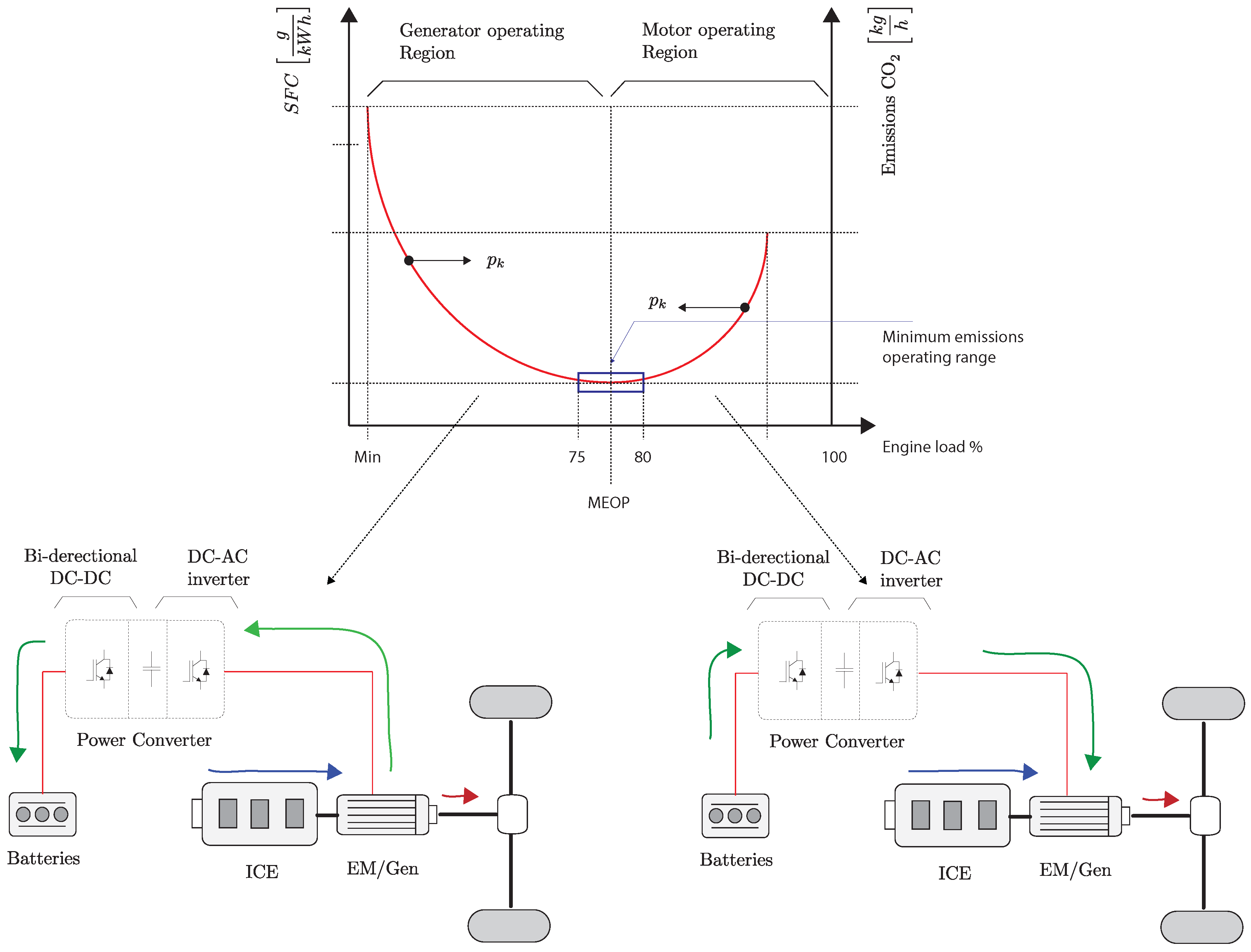
Both electric motor and combustion engine are sharing the power flow delivered to the drivetrain. The optimization strategy must ensure the MEOP of the combustion engine by controlling the power flow direction in the electric motor. For high load requirements the electric motor must supply the difference of power needed. On the other hand, for low load conditions the electric motor must absorbs the extra power. The power flow direction for both cases is shown in the Figure 2, also the emissions’ profile is depicted.

For the tandem configuration, the required torque $T_{req}$ at the drivetrain is

$$T_{req}=T_{ce}+T_e,$$

(1)

where $T_{ce}$ torque provided by the combustion engine, and $T_e$ is the torque developed by the EM.

2.1. Electric Machine Dynamics

The dynamics of the PMSM is described from the space vector representation in Equation (2)

$${\mathbf{v}}_s=R_s{\mathbf{i}}_{\mathbf{s}}+\frac{d}{dt}{\mathsf{\Psi }}_{\mathbf{s}},$$

(2)

where spatial vector components of voltage ${\mathbf{v}}_{\mathbf{s}}$; current ${\mathbf{i}}_{\mathbf{s}}$, and flux linkage ${\mathsf{\Psi }}_{\mathbf{s}}$ are 120° apart from each other.

Through a transformation $\mathcal{T}:\{a,b,c\}\to \{d,q,0^{\prime }\}$ given by Equation (3)

$$\mathcal{T}=\frac{2}{3}\left[\begin{array}{ccc}sin\theta & sin\theta -\frac{2\pi }{3}& sin\theta +\frac{2\pi }{3}\\ cos\theta & cos\theta -\frac{2\pi }{3}& cos\theta +\frac{2\pi }{3}\\ \frac{1}{2}& \frac{1}{2}& \frac{1}{2}\end{array}\right],$$

(3)

it is possible to describe the electrical dynamic in a rotating reference frame whose axes are named ($d-q$): direct and quadrature. In this case, the angle $\theta$ of the rotating reference frame is aligned with the permanent magnets flux linkage, therefore, the electrical dynamic is described by Equations (4) and (5):

$$v_s^d=R_s{i}_s^d+L_d\frac{d}{dt}{i}_s^d-p{\omega }_r{L}_q{i}_s^q,$$

(4)

$$v_s^q=R_s{i}_s^q+L_q\frac{d}{dt}{i}_s^q+p{\omega }_r{L}_d{i}_s^d+{\omega }_r{\psi }_m,$$

(5)

The torque developed by the machine in terms of the $d-q$ stator currents is expressed in Equation (6) as follows:

$$T_e=\frac{3}{2}p\left[{\psi }_m{i}_s^q+i_s^d{i}_s^q(L_d-L_q)\right]$$

(6)

Next, the fundamental principle of a three-level T-type inverter which drives the PMSM is described.

2.2. T-Type Inverter Fundamental Principle

The fundamental T-type cell is a T-array of four switching devices as ilustrated in Figure 3. Typically, IGBTs or MOSFETs are used for high-voltage, high-frequency switching operation. The T-type converter is capable to synthesize three output voltage levels per phase, by using three different switching states: $+;0;-$. Depending on the switching vector $S_x$ (which are presented in

Table 1. Switching states of the T-type inverter fundamental cell.

${\mathbf{S}}_{\mathbf{x}}$	${\mathbf{S}}_1$	${\mathbf{S}}_2$	${\mathbf{S}}_3$	${\mathbf{S}}_4$	${\mathbf{v}}_{\mathbf{xN}}$
+	1	1	0	0	$+v_{dc}/2$
0	0	1	1	0	0
-	0	0	1	1	$-v_{dc}/2$

) the output voltage can be expressed in terms of Equation (7)

$$v_{xN}=S_x\frac{v_{dc}}{2},$$

(7)

where $S_x$ represents the switching vector and $v_{xN}$ the output phase-neutral voltage for $x\in \{a,b,c\}$. The switching states are presented in Table 1 for a fundamental cell.

The total amount of switching states generated by three switching states and three phases is $N=3^3=27$. Nevertheless, there are redundant states that generate the same voltage level, thus the total active switching states reduces to 19. In Figure 4 the total active switches with the redundant vectors are represented in a orthogonal $\alpha -\beta$ reference frame.

dc-Link

The dc-link is formed by two capacitors clamped to a common neutral point N as depicted in Figure 3. The voltage dynamics to model each dc-link capacitor is described in terms of the neutral point current as

$$\frac{d}{dt}{v}_{c1}=\frac{1}{2C}{i}_o,$$

(8)

$$\frac{d}{dt}{v}_{c2}=-\frac{1}{2C}{i}_o,$$

(9)

where $i_o=i_{c1}-i_{c2}$ and C is the capacitance of both capacitors and satisfy that $C=C1=C2$. The neutral point current is common for the three-phase currents, hence

$$i_o=\sum _x{S}_{xo}{i}_x,$$

(10)

where $S_{xo}$ represents the switching states associated with the common neutral point N. Considering Table 1, the phase is connected to the neutral point only when $S_x=0$, In this way $S_{xo}=1$ when $S_x=0$, otherwise $S_{xo}=0$.

The main issue with this topology, and the multilevel converters in general, is that voltage drift between capacitors may occur, unbalancing the dc-link voltages. Within the 19 active vectors, if a majority of positive redundant switching states is selected the top capacitor tends to discharge, otherwise, if a majority of negative switching states is chosen the bottom capacitor tends to lose its charge.

2.3. Buck-Boost Converter Fundamental Principle

Aiming to regulate the dc-link voltage that fed the inverter a bi-directional Buck-Boost converter is switched, such that it maintains his dc voltage supply invariant against high-demand currents and regenerative periods.

The Buck-Boost converter is depicted in Figure 5. The stages of the converter are differentiated by the switching state of $Q_1$. If the switching state is ON, the inductor is directly connected to the source increasing its stored energy while the capacitor supplies power to the load. On the other hand, if the switching state is OFF, the inductor is isolated from the source and supplies its stored energy to the load and charges the capacitor. The Buck-Boost converter dynamic is presented in Equations (11) and (12)

$$\frac{d}{dt}{v}_c=\frac{(u-1)}{C}{i}_L-\frac{1}{C}{i}_r,$$

(11)

$$\frac{d}{dt}{i}_l=\frac{(1-u)}{L}{v}_c+\frac{u}{L}{v}_{in},$$

(12)

where u is the switching signal of the $Q_1$ with $u\in \{0,1\}$. $i_L$ is the inductor current and $v_c$ the capacitor voltage.

By averaging the ON and OFF time of the switching device, the output voltage is

$$v_{out}=\frac{D}{1-D}{v}_{in},$$

(13)

where D is the duty cycle of the converter and its defined by $D=t_{on}/(t_{on}+t_{off})$. The termn $\frac{D}{1-D}$ is known as the static gain of the converter, for $0.5<D<1$ the output voltage is greater than the input voltage, for $0<D<0.5$ the output voltage is less than the input voltage, and for $D=0.5$ the output and input voltages are equal. Therefore, manipulating the duty cycle D the required output voltage is achieved.

It is important to note that the Equation (13) considers a operation in Continuous Current Mode (CCM) in the inductor current and does not include the voltage ripple introduced by the switching devices.

3. Vehicle Dynamics

The main forces experienced by the vehicle are: aerodynamic drag, rolling resistance and acceleration resistance. Aerodynamic drag $\left(F_d\right)$ is the component of the force exerted by the air on the vehicle that is parallel and opposite to the direction of motion. Rolling resistance $\left(F_r\right)$ is the force resisting the motion when a body rolls on a surface. Finally, acceleration resistance $\left(F_a\right)$ can be defined as the proportion of inertia forces in the overall road resistance. Therefore, the vehicle road-load force $\left(F_t\right)$ is

$$F_t=F_d+F_r+F_a$$

(14)

The forces expressed above are not quite simple to compute. For this reason the Environmental Protection Agency (EPA) in the United Stated has conducted a series of experiments to express Equation (14) in terms of coefficients depending on the vehicle itself and its velocity [26,27]. Thus the vehicle road-load force can be expressed as

$$F_t=A+B\mathrm{v}+C{\mathrm{v}}^2$$

(15)

where v is the vehicle speed in m/s; and the A, B, and C coefficients are determined from the EPA testings for each vehicle. Typically, coefficient A correlates to the rolling resistance, C to the aerodynamic drag, and B to the rotational losses.

In order to move the vehicle, according to Newton’s law $\sum F=md\mathrm{v}/dt$. Hence, the traction force delivered by the vehicle is by calculated by

$$F_m=ma+F_t$$

(16)

where m is the total wight of the vehicle, and a its acceleration.

Vehicle Load Torque

The rotational equivalent of force is torque. Both quantities are related through the radius r of the wheels and the gears ratio g. Considering the traction force giving by Equation (15) and the vehicles force by Equation (16), the vehicle load toque is

$$T_l=\left(\frac{r}{g}\right)\left[A+B\mathrm{v}+C{\mathrm{v}}^2+ma\right]$$

(17)

Note that the load torque is equal to the required torque $T_{req}$ at the drivetrain.

4. Emissions Profile Model

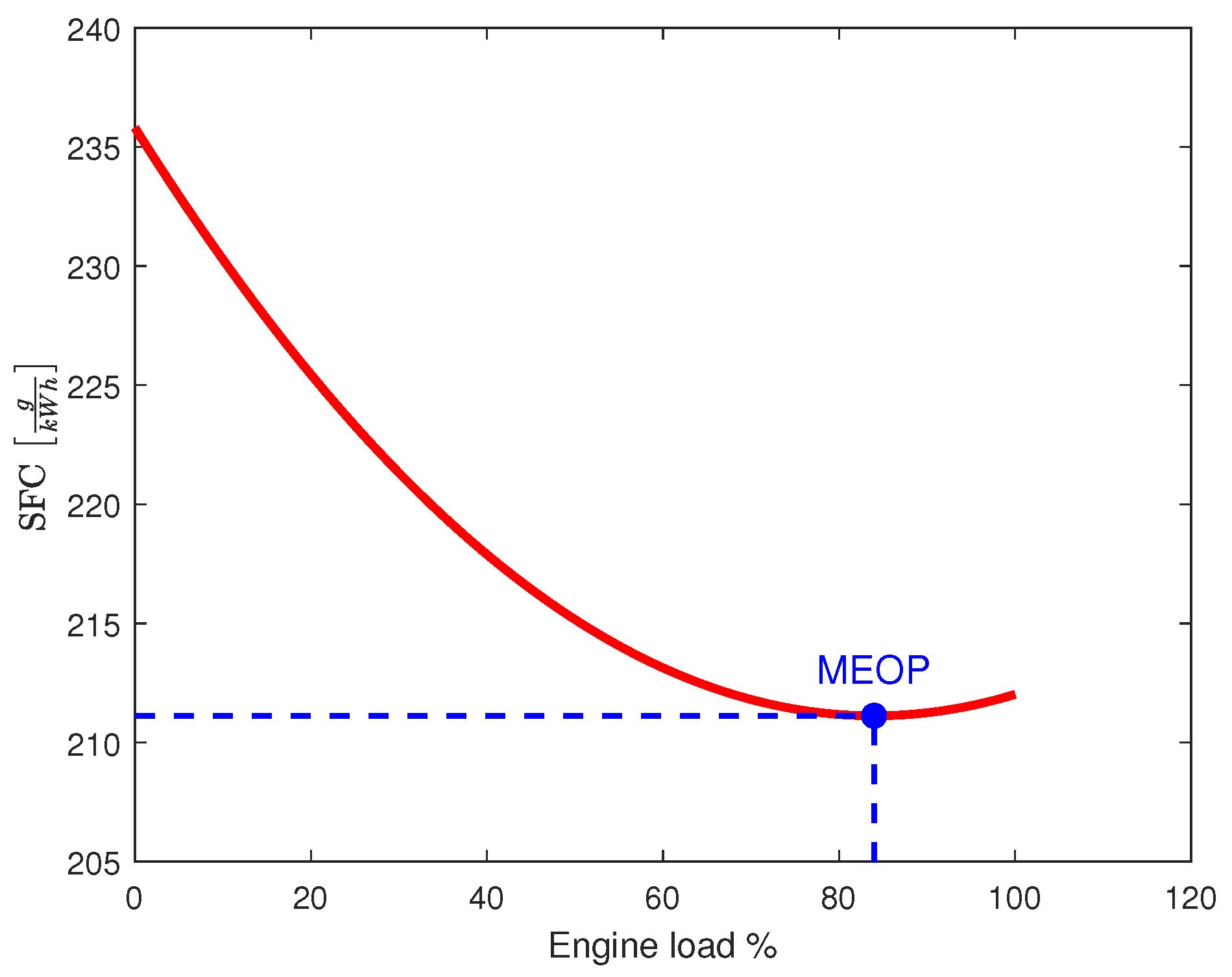
It is well known that the ICE produces toxic gas emissions. The emissions are generated during the process of converting chemical energy stored in the fuel into mechanical work. During the combustion process the emissions profile exhibits its maximum when operating the ICE at low and high loads [28]. The specific fuel consumption (sfc) requirements reach its lower value within the range of 75% to 85% of the engine Maximum Continuous Rating (MCR). In order to achieve the minimum emission point the combustion engine must be on the minimum sfc operation point, this point is defined as Minimum Emission Operating Point (MEOP).

It is possible to build the emissions model, which will be used in the optimization process. Given m data points ${\left\{x_i{y}_i\right\}}_{i=1}^m$ with $x_i$ given output power and $y_i$ corresponding CO${}_2$ emissions rate; the best fit polynomial for the CO${}_2$ emissions $f\left(x\right)$ could be developed using Equation (18) as:

$$f\left(x\right)=\sum _{k=0}^n{\alpha }_k{x}^{k}n<m-1$$

(18)

where ${\alpha }_k\forall k$ coefficients may be found by minimizing the least square error using Equation (19) as follows

$$A^{T}A\mathit{a}=A^T\mathit{y}$$

(19)

with the coefficients vector $\mathit{a}={[{\alpha }_0\dots {\alpha }_n]}^T$, the sample value vector $\mathit{y}={[y_0\dots y_n]}^T$, and A the Vandermonde matrix, given as in Equations (20) and (21).

$$A=\left[\begin{array}{ccccc}1& x_1& x_1^2& \dots & x_1^n\\ 1& x_2& x_2^2& \dots & x_2^n\\ ⋮& ⋮& ⋮& ⋮\\ 1& x_m& x_m^2& \dots & x_m^n\end{array}\right]\forall x_{i}i=1,\dots ,m$$

(20)

$$\mathit{a}={\left(A^{T}A\right)}^{-1}{A}^T\mathit{y}$$

(21)

Obtaining finally an n degree polynomial representing the CO${}_2$ emissions profile, as given in Equation (22).

$$f\left(x\right)=a_0+a_{1}x+a_2{x}^2+\dots +a_n{x}^n$$

(22)

Typically, the CO${}_2$ emission profile is a convex function with a local minimum within its operation area. Thus the MEOP can easily be found by solving

$$\frac{d}{dt}f\left(x\right)=0$$

for x within range of operation of the combustion engine.

In particular, the engines sfc profile used is depicted in Figure 6. The MEOP occurs at $84\%$ of the engine load with $211.1\left[\frac{g}{kWh}\right]$ of fuel consumption.

5. Optimization Strategy and Control Scheme

In this section the overall optimization strategy and control scheme is presented. The main two objectives of the whole system are the regulation of dc link voltage that fed the inverter, and the minimization of the emission exhaled by the combustion engine.

For the optimization strategy, an arbitrary optimization problem $\varphi$ is defined by Equations (23)–(26).

$$\varphi =\langle \mathcal{C},\mathcal{S},\nu ,f\left(x\right)\rangle ,$$

(23)

$$\mathcal{C}=x;x=\{x_0,\dots ,x_n\},$$

(24)

$$\mathcal{S}=x\pm \delta ,$$

(25)

$$\nu =min\left\{f\left(x\right){|}_{x\pm \delta }\right\},$$

(26)

where $\mathcal{C}$ corresponds to the set of candidate solutions $\mathcal{S}$, with $\mathcal{S}\subseteq \mathcal{C}$ of the optimization problem, $f\left(x\right)$ is the objective function, $\nu$ indicates the optimization sense; x corresponds to the system state and $\delta$ to the variation of the state introduced by the search direction of the optimization strategy.

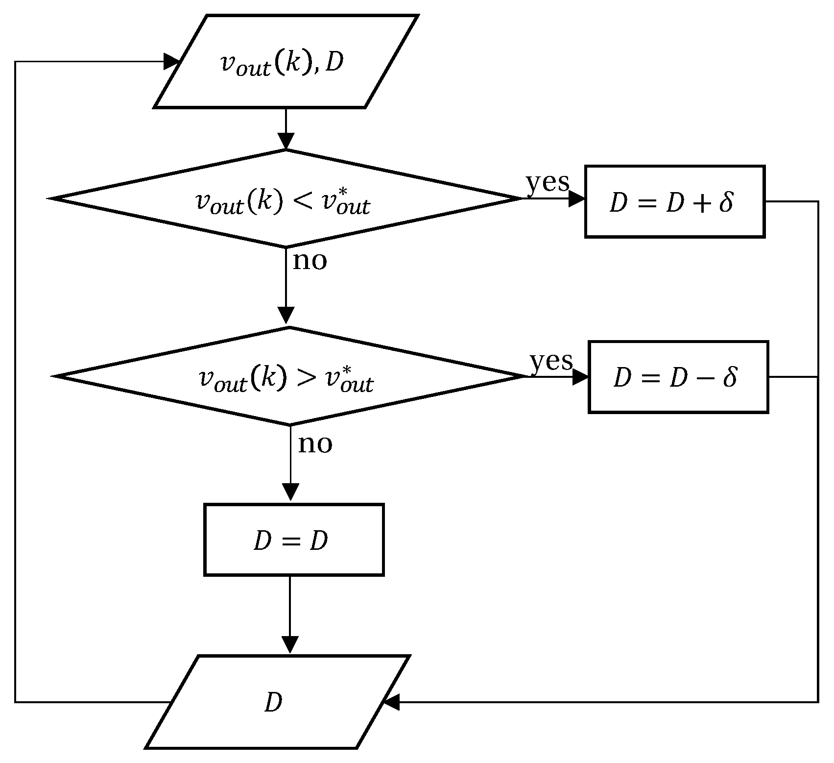
The voltage regulation of the Buck-Boost converter, for simplicity, is achieved through a Perturb & Observe-based optimization algorithm that, according to the output voltage measurement, chooses whether the duty cycle increases, decreases, or maintains its value. The strategy is designed to move the duty cycle such that the output voltage stays as near as possible to a fixed reference. The algorithm flowchart is shown in Figure 7. First the duty cycle D and the output voltage $v_{out}$ are sampled, if the voltage is below a reference $v_{out}^{*}$ the duty cycle is increased by a constant value $\delta$, if it is above the reference D is decreased by $\delta$, else the duty cycle remains the same.

Alternatively, to minimize the emissions the optimization strategy is designed to move the operational point of the ICE towards the MEOP by controlling the power flow direction in the EM, by means of a MPC scheme. The predicted currents, and hence predicted electrical torque, that minimize the combustion engine emissions according to a cost function are applied. The rate of change of the emissions respect to the torque developed by the internal combustion engine can be assumed to be invariable within one sample time $0\le t\le T_s$, with $T_s$ the control platform sampling time.

5.1. Model Predictive Control Scheme

In order to control the dc-link voltage and the electrical drive, and thus the emissions, a MPC strategy is proposed using optimum voltage space vectors given by the T-type. The total number of voltage vectors is $N=3^3=27$, and by using all the non-zero redundant voltage vectors in the prediction scheme the dc-link voltage balance is achieved. The model under prediction is given by Equations (4), (5), (8) and (9). Discretizing the currents and voltages using the forward Euler method, the predicted currents and voltages within one horizon of prediction are expressed in Equations (27)–(30) as follows:

$$i_s^d(k+1)=\left(1-\frac{T_s}{L_s}{R}_s\right)i_s^d\left(k\right)+{\omega }_k{T}_s{i}_s^q\left(k\right)+\frac{T_s}{L_s}{v}_s^d\left(k\right),$$

(27)

$$i_s^q(k+1)=\left(1-\frac{T_s}{L_s}{R}_s\right)i_s^q\left(k\right)-{\omega }_k{T}_s{i}_s^d\left(k\right)+\frac{T_s}{L_s}{v}_s^q\left(k\right)-\frac{T_s}{L_s}{\psi }_m{\omega }_k,$$

(28)

$$v_{c1}(k+1)=v_{c1}\left(k\right)+\frac{1}{2C}{i}_o\left(k\right)T_s,$$

(29)

$$v_{c2}(k+1)=v_{c2}\left(k\right)-\frac{1}{2C}{i}_o\left(k\right)T_s,$$

(30)

where the predictions given by $(k+1)$ depends on the current state $\left(k\right)$. The discretization occurs at sampling time $T_s$. The prediction of the electrical torque, and therefore the combustion engine torque, is obtained by substituting Equations (27) and (28) into Equation (6), and then into Equation (1), in this way Equation (31) is obtained.

$$T_{ce}(k+1)=T_{req}\left(k\right)-\frac{3}{2}p\left[{\psi }_m{i}_s^q(k+1)+i_s^d(k+1)i_s^q(k+1)(L_d-L_q)\right].$$

(31)

For Equations (27) and (28) the converters output voltage in the $\left(k\right)$ state is given by $v_s^{\left(dq\right)}\left(k\right)=\widehat{f}(S_N,v_{dc})$, with $\widehat{f}(S_N,v_{dc})$ a non-linear function depending on the switching state $S_N$ and the total dc-link voltage $v_{dc}$ in the $\left(k\right)$ state.

Likewise, in Equations (29) and (30) the neutral point current $i_o\left(k\right)$ is given as $i_o\left(k\right)=\widehat{g}(S_N,i_s)$, with $\widehat{g}(S_N,i_s)$ a non-linear function depending on the switching state $S_N$ and the load current $i_s$ in the $\left(k\right)$ state, as presented in Equation (10).

The cost function g to be minimized includes the error between the predicted combustion engine torque and the MEOP; the difference between the dc-link voltages; and a saturation function according to the constrains of the model. As given in Equation (32)

$$g=|MEOP-T_{ce}(k+1)|+\widehat{h}\left(i_s^d(k+1),i_s^q(k+1)\right)+\lambda |v_{c1}(k+1)-v_{c2}(k+1)|$$

(32)

where $\widehat{h}$ corresponds to the saturation function on the maximum stator currents, and $\lambda$ is a weighting factor in the dc-link voltage balancing. The control objective $\mathcal{J}$ is to minimize the cost function g as shown in Equation (33).

$$\mathcal{J}=min\left\{g\right\},$$

(33)

It is evaluated for $N-2=25$ switching states, excluding the two zero redundant voltage vectors since they do not contribute tho the charge and discharge of both capacitors. The flowchart of the MPC strategy is represented in Figure 8.

Finally, the overall optimization and control scheme implementation is represented in Figure 9.

5.2. Convergence of the MPC Algorithm

The MPC optimization approximates an infinite-time problem by solving over a discrete finite horizon N. Lets extend the optimization problem defined in Equation (33) as given in Equation (34)

$$minJ(x\left(k\right),u\left(k\right))=\sum _{\ell =0}^{N}d(z(k+\ell |k),\mathcal{T}(\ell ))$$

(34)

The optimization problem is subjected to discrete state space description of the dynamic system given in Equation (35)

$$\left\{\begin{array}{c}x(k+\ell +1|k)=Ax(k+\ell \left|k\right)+Bu(k+\ell |k)\hfill \\ \\ y(k+\ell |k)=Cx(k+\ell \left|k\right)+Du(k+\ell |k)\hfill \\ \\ z(k+\ell |k)=Ex(k+\ell \left|k\right)+Fu(k+\ell |k)\hfill \end{array}\right.$$

(35)

where $z\left(k\right)$ corresponds the tracking output to converge to a bounded target set $\mathcal{T}$ as $k\to N$ and $d\left(z\right(k+\ell \left|k\right),\mathcal{T}(\ell ))$ to the metric given from each element of the tracking output set $z(k+\ell )$ to each target set element $\mathcal{T}(\ell )$ as given in Equation (36)

$$d\left(z\right(k+\ell \left|k\right),\mathcal{T}(\ell ))=min|\left|z\right(\ell )-\mathcal{T}(\ell \left)\right||$$

(36)

If the optimization problem $minJ\left(x\right(k),u(k\left)\right),\forall k>0$ has a feasible solution for the state variable $x\left(k\right)$ for any control action $u\left(k\right)$, the the optimization problem is feasible and converges to the global optimum [29], and as a consequence, the tracking output $z\left(k\right)$ converges to the target set $\mathcal{T}$ within a finite set of samples N as $k\to N$ [30].

6. Results

Simulation and Hardware-In-the-Loop results of the proposed optimization strategy are presented in this section. The complete system analysis is done through PLECS and then validated with the real-time platform RT-Box. For analysis purposes the simulation and the real-time validation take into account the same scenarios.

As previously mentioned, the HWFET drive cycle was used to evaluate the emissions of the hybrid vehicle. For simulation purposes only the most critical seconds of the driving cycle are considered. Between seconds 290 and 310 the highest $d\mathrm{v}/dt$ occurs. The speed and load torque at which the algorithm is tested are depicted in Figure 10. The EPA Hybrid vehicle parameters are in

Table 2. EPA Hybrid Vehicle Parameters.

Parameter	Value
Weight	1531 [kg]
A	82.3 [N]
B	0.222 [N/ms${}^{-1}$]
C	0.403 [N/m${}^2$s${}^{-2}$]
Gear ratio	3.04 [−]
Wheel radius	0.313 [m]

, as a benchmark, parameters similar to a 2015 Toyota Prius [27] were used.

The parameters used for the simulation and the HIL validation are presented in

Table 3. Parameter used for the simulation.

	Parameter	Value
Converter Parameters
$V_{dc}$	dc-Link voltage	800 [V]
$C$	dc-Link capacitor	5000 [$\mathsf{\mu }$F]
PMSM Parameters
$R_s$	Stator resistance	0.005 [$\Omega$]
$L_d$	direct-axis Stator inductance	0.3 [mH]
$L_q$	quadrature-axis Stator inductance	0.3 [mH]
${\psi }_m$	PM Flux Linkage	0.192 [Wb]
p	Pole pairs	4 [−]
Sampling Time
$T_{disc}$	Base system discretization time	5 [$\mathsf{\mu }$s]
$T_s$	MPC Sampling time	10 [$\mathsf{\mu }$s]
$T_{dc}$	Buck-Boost optimization algorithm	1 [ms]
MPC	Prediction Horizon	One
Hardware In the Loop	Processing capability	95%

. The whole simulation has been implemented in PLECS, the drive system and the PMSM were modeled using specialized blocks, the overall control scheme for the drive were written in C code.

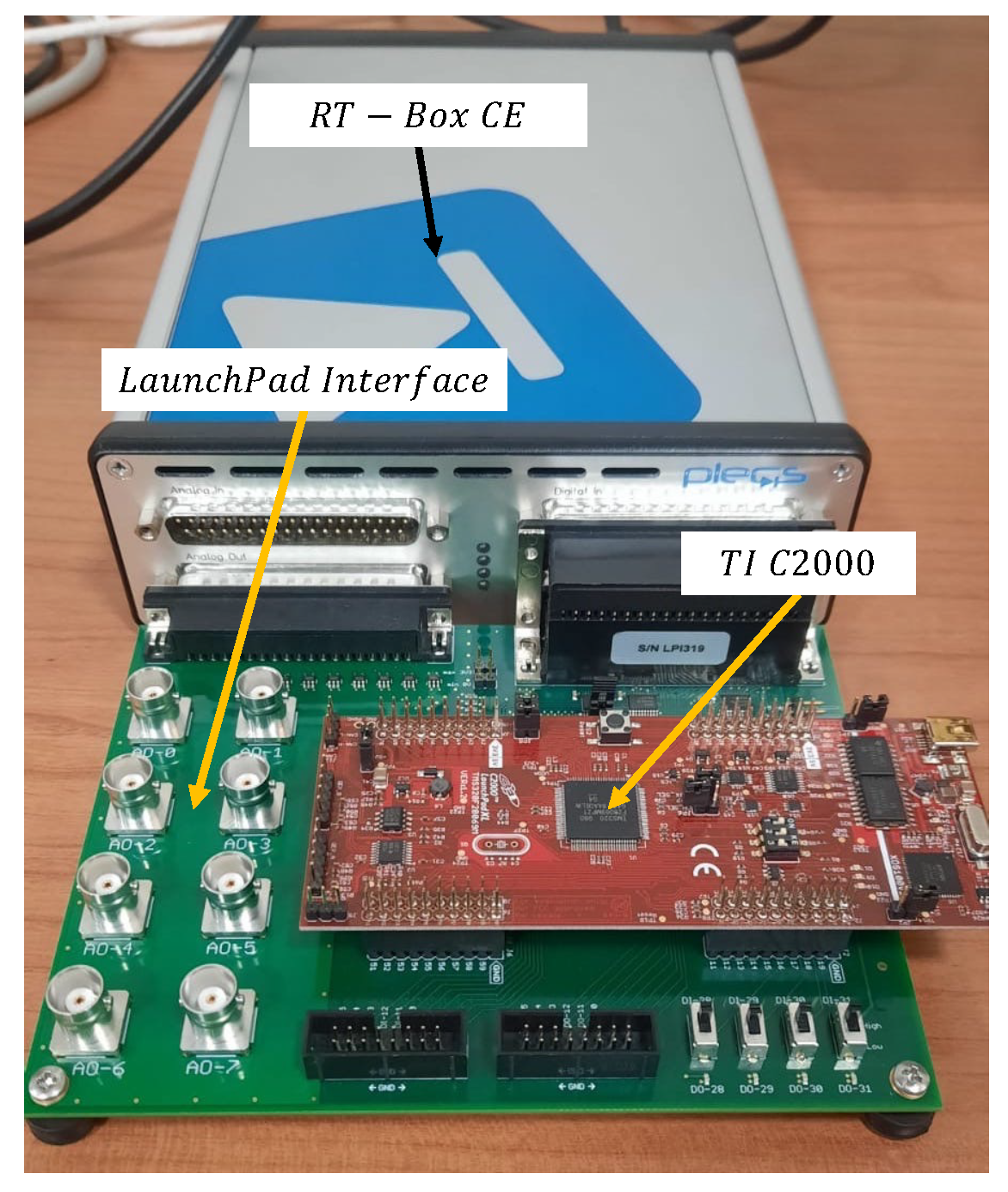
HIL verification was carried out in a Plexim RT-Box CE HIL, running a TI C2000 micro-controller as shown in Figure 11, various analog outputs signals were captured and visualized through an external oscilloscope using the RT-Box LaunchPad Interface.

Offline simulation and HIL validation consider the same scenario for analysis purposes. Step-type changes are applied for the required torque at the HEV drivetrain, in such way that the electric machine goes from operating in motor mode to generator mode and vice versa, changing the direction of the power flow in order to reach MEOP of the combustion engine.

6.1. Simulation Results

The first simulation results presented are the torques at the drive train and the emissions of the ICE in the critical portion of the driving cycle. In Figure 12, the EM changes its operating point allowing the ICE to work at its MEOP, regardless of drive cycle torque demand. Furthermore, in Figure 13, the instantaneous sfc with and without the optimization strategy are shown. The optimization strategy moves the sfc to the MEOP, reducing gas emissions to its minimum. For the case without the optimization strategy, the instantaneous sfc reflects a high fuel consumption exhaling a greater amount of CO${}_2$ into the atmosphere.

According to EPA [31], the CO${}_2$ emissions per gallon of gasoline of a passenger vehicle are 8887 g/gal, equivalent to 2.34 kg/L. Considering a 73 kW vehicle on highway, the CO${}_2$ emissions of the HEV with and without the optimization strategy are in

Table 4. CO${}_2$ emissions on Highway.

Engine Condition	Specific Fuel Consumption	CO${}_2$ Emissions
	[g/kWh]	[kg/h]
100% load	212.0	51.0
75% load	211.4	50.7
50% load	215.1	51.7
25% load	223.3	53.6
Emission reduction strategy	211.1	50.7

. For the emissions without the optimization strategy only the ICE delivers power due to the highway operation, different engine load conditions were taken into account. For a near constant speed on highway the engine at high loads remains close to the MEOP, therefore the decrease in emissions does not seem much. However, emissions are mainly reduced in transients periods of acceleration and deceleration where the sfc of the engine moves away from the MEOP.

The second simulation results present a dynamic operation under two different scenarios. A high torque step from 60 Nm to 174 Nm was applied to vehicle drivetrain. After the high torque demand took place, an opposite direction high torque was performed from 120 Nm to −40 Nm. The two sudden step changes change the EM operating mode between Motor and Generator; and vice versa. Figure 14 shows the dynamic response of the vehicle, the EM currents and the dc-link voltages. The performance of the optimization strategy is observed. The combustion engine torque converges to the MEOP, when increasing the required torque the electrical motor changes the operation region from generator to motor, supplying torque such that the torque developed by the combustion engine reaches MEOP and stays in its vicinity. On the other hand, the dc-voltage stays near invariant when the load increased due to effectiveness of the Buck-Boost voltage optimization algorithm and the MPC voltage balance strategy. The maximum voltage ripple is about 5% and the balance is such that its difficult to differentiate both voltages since they are superimposed assuring voltage balancing, with near zero voltage drift. The MPC algorithm is controlling both, the stator currents and the voltage balance of the dc-link capacitors successfully.

6.2. Hardware-in-the-Loop Validation

In the HIL validation the same scenario was taken into account. The whole system is virtualized and waveforms of interest are observed through an oscilloscope from the Launchpad Interface, the HIL set up is shown in Figure 15 for the stator currents $\alpha -\beta$ Figure 15a and torques at the drivetrain Figure 15b.

For the real-time Hardware-In-the-Loop simulation, the previous scenario of step up and step down torque was taken into account. The torques at the drive train, stator currents, and dc-link voltages for the step-up scenario are in Figure 16, while for the step-down, the same waveforms are shown in Figure 17. The torque of the combustion engine reaches the MEOP in a high magnitude abrupt torque demand operation, guaranteeing a minimum CO${}_2$ emission, as shown in the offline simulation, validating all the results obtained previously. The waveforms of the currents exhibit a sinusoidal pattern, the amplitude change is almost instantaneous due to the fast response of the control algorithm, the phase change of the currents follows the same behavior as the offline simulation. Finally, the voltages of the DC link capacitors present low ripple without voltage imbalance between them, validating the results obtained previously.

7. Discussion

The optimization strategy ensures the ICE developed torque operating within minimum emissions operational region. On the other hand, the electric drive is capable to operate in both motor and generator regions. In the motor operation region the electromechanical torque is used to move the combustion engine operation point into it’s minimum emissions zone, while in the generator operational region the residual torque of the combustion engine is used as regeneration. The MPC strategy ensures optimum performance in both motor and generator operation regions, ensuring full current reference tracking capability, simultaneously, balance the voltage of the T-type dc-link capacitors, reducing voltage drift. The Buck-Boost voltage optimization algorithm ensure a near constant fed to the dc-link, decreasing the total ripple of the voltages, hence on the current as well.

Finally, the results were validated using HIL real-time simulation modelling the entire system and its control, the similitude between the offline and the HIL simulation validates the optimization strategies proposed.

8. Conclusions

Emissions were reduced with the optimization algorithm implemented on a tandem HEV drive, thus ensuring the Internal Combustion Engine on its most fuel efficient operational point, reducing total CO${}_2$ emissions. This fact also proves the versatility and capability of the MPC constraints to deal with the optimization problem. The unbalance of the T-type dc-link voltages was solved by including the prediction of the capacitors voltages in the cost function, thus the torque and voltage balancing are controlled by the MPC algorithm. The Buck-Boost optimization algorithm sets the dc-link fed voltage near constant, providing high-quality dc supply to the inverter stage. Results were validates by means of HIL real-time simulation, where both HEV and controllers were discrete implemented using a dedicated external microprocessor TI C2000. Hardware in the Loop real-time simulation provides near real setup implementation to test the effectiveness of the overall control scheme. MPC has proven to be a powerful and versatile control strategy to deal with multi-objective control problems, as presented in this work, being capable to ensure full electric drive control, with dc-link voltage balancing capability and also ensuring minimum emissions operation of the internal combustion engine, becoming a very interesting alternative to classic control approach for its application on Hybrid Electric and Full Electric Vehicles.

References

- Sthel, M.S.; Tostes, J.G.R.; Tavares, J.R. Current energy crisis and its economic and environmental consequences: Intense human cooperation. Nat. Sci. 2013, 5, 244–252. [Google Scholar] [CrossRef]
- Yong, J.Y.; Ramachandaramurthy, V.K.; Tan, K.M.; Mithulananthan, N. A review on the state-of-the-art technologies of electric vehicle, its impacts and prospects. Renew. Sustain. Energy Rev. 2015, 49, 365–385. [Google Scholar] [CrossRef]
- Du, J.; Ouyang, M. Review of Electric Vehicle Technologies Progress and Development Prospect in China. World Electr. Veh. J. 2013, 6, 1086–1093. [Google Scholar] [CrossRef]
- Un-Noor, F.; Padmanaban, S.; Mihet-Popa, L.; Mollah, M.; Hossain, E. A Comprehensive Study of Key Electric Vehicle (EV) Components, Technologies, Challenges, Impacts, and Future Direction of Development. Energies 2017, 10, 1217. [Google Scholar] [CrossRef]
- Chan, C.C.; Chau, K.T. Modern Electric Vehicle Technology; Oxford University Press: New York, NY, USA, 2001; p. 318. [Google Scholar]
- Chau, K.T. Electric Vehicle Machines and Drives Design, Analysis and Application; John Wiley and Sons, Inc.: Hoboken, NJ, USA, 2015. [Google Scholar]
- Chau, K.T.; Jiang, C.; Han, W.; Lee, C.H.T. State-of-the-art electromagnetics research in electric and hybrid vehicles (invited paper). Prog. Electromagn. Res. 2017, 159, 139–157. [Google Scholar] [CrossRef]
- Lopes, J.A.P.; Soares, F.J.; Almeida, P.M.R. Integration of Electric Vehicles in the Electric Power System. Proc. IEEE 2011, 99, 168–183. [Google Scholar] [CrossRef]
- Dyke, K.J.; Schofield, N.; Barnes, M. The Impact of Transport Electrification on Electrical Networks. IEEE Trans. Ind. Electron. 2010, 57, 3917–3926. [Google Scholar] [CrossRef]
- Liu, C.; Chau, K.T.; Wu, D.; Gao, S. Opportunities and Challenges of Vehicle-to-Home, Vehicle-to-Vehicle, and Vehicle-to-Grid Technologies. Proc. IEEE 2013, 101, 2409–2427. [Google Scholar] [CrossRef]
- Emadi, A.; Williamson, S.; Khaligh, A. Power electronics intensive solutions for advanced electric, hybrid electric, and fuel cell vehicular power systems. IEEE Trans. Power Electron. 2006, 21, 567–577. [Google Scholar] [CrossRef]
- Li, Y.; Yu, G.; Liu, J.; Deng, F. Design of V2G auxiliary service system based on 5G technology. In Proceedings of the 2017 IEEE Conference on Energy Internet and Energy System Integration (EI2), Beijing, China, 26–28 November 2017; IEEE: Piscataway, NJ, USA, 2017. [Google Scholar] [CrossRef]
- Bonetto, R.; Sychev, I.; Zhdanenko, O.; Abdelkader, A.; Fitzek, F.H. Smart Grids for Smarter Cities. In Proceedings of the 2020 IEEE 17th Annual Consumer Communications & Networking Conference (CCNC), Las Vegas, NV, USA, 10–13 January 2020; IEEE: Piscataway, NJ, USA, 2020. [Google Scholar] [CrossRef]
- Livint, G.; Horga, V.; Ratoi, M.; Albu, M. Control of Hybrid Electrical Vehicles. In Electric Vehicles—Modelling and Simulations; InTech: London, UK, 2011. [Google Scholar] [CrossRef]
- Mashadi, B. Vehicle Powertrain Systems; Wiley: Hoboken, NJ, USA, 2012. [Google Scholar]
- Gao, D.W.; Mi, C.; Emadi, A. Modeling and Simulation of Electric and Hybrid Vehicles. Proc. IEEE 2007, 95, 729–745. [Google Scholar] [CrossRef]
- Hu, X.; Zhang, X.; Tang, X.; Lin, X. Model predictive control of hybrid electric vehicles for fuel economy, emission reductions, and inter-vehicle safety in car-following scenarios. Energy 2020, 196, 117101. [Google Scholar] [CrossRef]
- Oncken, J.; Chen, B. Real-Time Model Predictive Powertrain Control for a Connected Plug-In Hybrid Electric Vehicle. IEEE Trans. Veh. Technol. 2020, 69, 8420–8432. [Google Scholar] [CrossRef]
- Zhang, F.; Hu, X.; Liu, T.; Xu, K.; Duan, Z.; Pang, H. Computationally Efficient Energy Management for Hybrid Electric Vehicles Using Model Predictive Control and Vehicle-to-Vehicle Communication. IEEE Trans. Veh. Technol. 2021, 70, 237–250. [Google Scholar] [CrossRef]
- Vu, T.M.; Moezzi, R.; Cyrus, J.; Hlava, J.; Petru, M. Parallel Hybrid Electric Vehicle Modelling and Model Predictive Control. Appl. Sci. 2021, 11, 10668. [Google Scholar] [CrossRef]
- Serpi, A.; Porru, M. An MPC-based Energy Management System for a Hybrid Electric Vehicle. In Proceedings of the 2020 IEEE Vehicle Power and Propulsion Conference (VPPC), Gijon, Spain, 18 November–16 December 2020; IEEE: Piscataway, NJ, USA, 2020. [Google Scholar] [CrossRef]
- Kouro, S.; Malinowski, M.; Gopakumar, K.; Pou, J.; Franquelo, L.G.; Wu, B.; Rodriguez, J.; Pérez, M.A.; Leon, J.I. Recent Advances and Industrial Applications of Multilevel Converters. IEEE Trans. Ind. Electron. 2010, 57, 2553–2580. [Google Scholar] [CrossRef]
- Tran, H.N.; Nguyen, T.D. Predictive voltage controller for T-type NPC inverter. In Proceedings of the 2016 IEEE Region 10 Conference (TENCON), Singapore, 22–25 November 2016; IEEE: Piscataway, NJ, USA, 2016. [Google Scholar] [CrossRef]
- Xing, X.; Chen, A.; Zhang, Z.; Chen, J.; Zhang, C. Model predictive control method to reduce common-mode voltage and balance the neutral-point voltage in three-level T-type inverter. In Proceedings of the 2016 IEEE Applied Power Electronics Conference and Exposition (APEC), Long Beach, CA, USA, 20–24 March 2016; IEEE: Piscataway, NJ, USA, 2016. [Google Scholar] [CrossRef]
- US-Environmental Protection Agency (EPA). EPA Highway Fuel Economy Test Cycle (HWFET). Available online: https://dieselnet.com/standards/cycles/hwfet.php#:~:text=Time%2Dspeed%20data%20points%20%7C%2010,CFR%20600%2C%20subpart%20B%5D%20 (accessed on 30 December 2022).
- Hayes, J.G.; Goodarzi, G.A. Electric Powertrain Energy Systems, Power Electronics and Drives for Hybrid, Electric and Fuel Cell Vehicles; Wiley & Sons, Incorporated, John: Hoboken, NJ, USA, 2017; p. 560. [Google Scholar]
- US-Environmental Protection Agency (EPA). Data on Cars Used for Testing Fuel Economy. Available online: https://www.epa.gov/compliance-and-fuel-economy-data/data-cars-used-testing-fuel-economy (accessed on 30 December 2022).
- Pietracho, R.; Kasprzyk, L.; Burzynski, D. Electrical propulsion systems in vehicles—An overview of solutions. In Proceedings of the 2019 Applications of Electromagnetics in Modern Engineering and Medicine (PTZE), Janow Podlaski, Poland, 9–12 June 2019; IEEE: Piscataway, NJ, USA, 2019. [Google Scholar] [CrossRef]
- Maciejowski, J.M. Predictive Control with Constraints; Prentice Hall: Hoboken, NJ, USA, 2002; p. 352. [Google Scholar]
- Mayne, D.; Rawlings, J.; Rao, C.; Scokaert, P. Constrained model predictive control: Stability and optimality. Automatica 2000, 36, 789–814. [Google Scholar] [CrossRef]
- US-Environmental Protection Agency (EPA). Greenhouse Gas Eissions from a Typical Passenger Vehicle. Available online: https://www.epa.gov/greenvehicles/greenhouse-gas-emissions-typical-passenger-vehicle#:~:text=typical%20passenger%20vehicle%3F-,A%20typical%20passenger%20vehicle%20emits%20about%204.6%20metric%20tons%20of,8%2C887%20grams%20of%20CO2 (accessed on 23 February 2023).
Figure 1.
HEV configuration.
Figure 2.
Specific fuel consumption of a HEV and power flow direction.
Figure 3.
T-type fundamental cell.
Figure 4.
Switching states and voltage vectors of the three-phase T-type inverter.
Figure 5.
Buck-Boost Converter.
Figure 6.
Specific fuel consumption of the ICE.
Figure 7.
Buck-Boost voltage optimization strategy flowchart.
Figure 9.
Overall optimization strategy and control scheme.
Figure 10.
Critical speed and torque points.
Figure 11.
RT-Box CE with the Launchpad Interface.
Figure 12.
Torque at the HEV drivetrain.
Figure 13.
Instantaneous sfc with and without the optimization strategy.
Figure 14.
Dynamic operation of Torques at the drive train, currents, and dc-voltages.
Figure 15.
(a) Stator currents HIL validation. (b) Torques from Minimum emission optimization algorithm HIL validation.
Figure 16.
HIL dynamic response against step up high torque demand. (a) Torques at the drivetrain. (b) Currents. (c) dc-Link voltages.
Figure 17.
HIL dynamic response against step down high torque demand. (a) Torques at the drivetrain. (b) Currents. (c) dc-Link voltages.