Article

Multi-Inverter Resonance Modal Analysis Based on Decomposed Conductance Model

State Key Laboratory of Alternate Electrical Power System with Renewable Energy Sources, School of Electrical and Electronic Engineering, North China Electric Power University, Beijing 102206, China
*
Author to whom correspondence should be addressed.
Electronics 2023, 12(5), 1251; https://doi.org/10.3390/electronics12051251
Submission received: 1 February 2023 / Revised: 28 February 2023 / Accepted: 2 March 2023 / Published: 5 March 2023
(This article belongs to the Special Issue Application of Power Electronics Technology in Energy System)

Abstract

:
The Norton equivalent model based on the transfer function and the frequency domain analysis method for inverter resonance analysis lacks a comprehensive analysis of the resonant characteristics, and more information about the resonant key components and the degree of participation cannot be obtained. In this paper, a decomposed conductance model is proposed to characterize the resonance characteristics of the multi-inverter grid-connected system and the effect of the equivalent control link of the inverter on the resonance in more detail by combining the modal analysis method and the sensitivity analysis method. Firstly, based on αβ coordinates, the conductance division is carried out for the dual-loop inverter control link with the voltage external loop and current internal loop using capacitor-current feedback damping, and the inverter model based on the decomposition conductance is derived. The mathematical model of the multi-inverter grid-connected system is then established. Secondly, the resonance characteristics of the system are analyzed by combining the modal and frequency domain analysis methods when the number of inverters, inverter parameters, and grid-side impedance are changed. Thirdly, the degree of involvement of the system components, especially the equivalent control link of the inverter in resonance conditions, is determined in combination with the proposed model and the sensitivity analysis method, which is the basis for proposing an effective suppression strategy. Finally, a simulation model is built to verify the proposed method and the analysis results.

1. Introduction

With the increasing proportion of new energy sources, the high proportion of electronic devices in power systems will be realized in the near future [1,2]. As an important interface between new energy and the power grid, the inverter has also caused much concern [3].
Nowadays, it is more and more common for multi-inverters to be connected to the power grid together [4]. As the number of grid-connected inverters increases, the interactive coupling between the grid-connected inverters and the power grid becomes more sophisticated [5,6], while the operating characteristics of the inverters have a greater impact on the stability of the power grid [7]. In [8,9], the dynamic and power losses of the converter were decreased by using the switched capacitor structure. In [10], an inverter topology is proposed to decrease the leakage current, which can increase efficiencies. In [11], the impedance analysis method was introduced to the grid-connected inverter system, where the power grid is equated as a series of an ideal voltage source and impedance and the grid-connected inverter is modeled as a series of a current source and impedance, which is used for correlation analysis of the system’s harmonic stability. In [12], the method is extended to a multi-inverter grid-connected system by considering the output conductance of other inverters and the conductance of the grid passive components as a whole for stability analysis; however, this method requires detailed transfer function models of the components, which can be quite computationally complicated with higher inverter dimensions [13,14]. In [15], the resonant stability domain criterion considering the influence of grid impedance and grid background harmonics and its optimal design scheme were established, and in [16], the relationship among the number of inverters connected to the power grid, filter parameters, and grid impedance was studied, and the larger the grid equivalent impedance and the more inverters connected in parallel, the more the resonant frequency of the system decreased.
In [17], a multi-inverter homodyne equivalence model was developed to quantify the degree of interaction between the original system and the added inverters, and this model was used to evaluate the effect of the interaction on the damping characteristics. In [18], a mechanical conductance model of a multi-virtual synchronous motor grid-connected system is constructed based on the active-frequency control loop to study the power-frequency oscillation characteristics under different parameters. In [19], a harmonic model of a large PV field station was established with the underground cables, field station transformers, and other equipment taken into account, and it was concluded that the LCL filter and the cables would each produce two resonant bands. However, the above literature still analyzes the system using the traditional Norton equivalent model, which is difficult to comprehensively reflect the response characteristics of the inverter and the grid.
In [20], modal analysis was applied to the resonance characteristics analysis of power systems, which can determine important information such as the resonance center and the participation of components in the resonance, effectively solving the problems of complex calculation processes and the low amount of response information of traditional spectrum analysis. In [21,22,23], resonant modal analysis was carried out for multi-inverter grid-connected systems, and the impedance model of the system was established to study the resonant interaction between the inverter and the power grid. However, there are few studies on the effective suppression of resonance by analyzing the degree of involvement of the key components of the system in resonance.
In this paper, based on the αβ coordinates, the conductance division of the double-loop inverter control link with capacitor-current feedback damping is carried out, and the inverter impedance model based on the decomposition conductance method is proposed. The mathematical model of the multi-inverter grid-connected system is established based on the decomposition conductance model. Also, the resonance characteristics of the system are analyzed by combining the modal and frequency domain analysis methods when the number of inverters, inverter parameters, and grid-side impedance are changed, and then the degree of participation of each component of the system in resonance is determined by sensitivity analysis and an effective suppression strategy is proposed. Finally, a simulation model was built to verify the resonance characteristics of the system.

2. Modal Analysis Method

The modal analysis method is a method introduced by dynamics and extended to the resonance analysis of electrical power systems. Assuming that the system occurs in parallel resonance and the resonant frequency is f, then the nodal voltage equation of the system is given in (1).
U f = Y f 1 I f
where Uf is the node voltage vector, Yf is the node derivative matrix with resonant frequency f, and If is the node current vector.
The decomposition of the nodal derivative matrix is given in Equation (2).
Y f = L Λ T
where L is the left eigenvector matrix, T is the right eigenvector matrix, and Ʌ is the diagonal matrix of eigenvalues. Equation (3) can be obtained from (1) and (2).
U f = L Λ 1 T I = L Λ 1 V
T U f = Λ 1 T I = J
where V is the modal voltage vector and J is the modal current vector, which are related as in Equation (5):
[ U f 1 U f 2 U f n ] = [ λ f 1 1 0 0 0 λ f 2 1 0 0 0 λ f n 1 ] [ J f 1 J f 2 J f n ]
[ U f 1 U f 2 U f n ] = λ m 1 [ L 1 m T m 1 L 1 m T m 2 L 1 m T m n L 2 m T m 1 L 2 m T m 2 L 2 m T m n L n m T m 1 L n m T m 2 L n m T m n ] [ I f 1 I f 2 I f n ]
The reciprocal of the eigenvalue is defined as the modal impedance of the system, and the smallest eigenvalue corresponds to the critical mode of the system. The resonance position can be judged based on the modal impedance because a very small modal current can also produce a large modal voltage. It can be seen that the modal impedance in this mode is much larger than the other modal impedances with a critical mode m from Equation (6).
The modal resonance can be characterized by the diagonal elements of the matrix of the above equation for its observability and excitability, which can also be called the participation factor, and the center of resonance can be determined by the calculation of the participation factor.

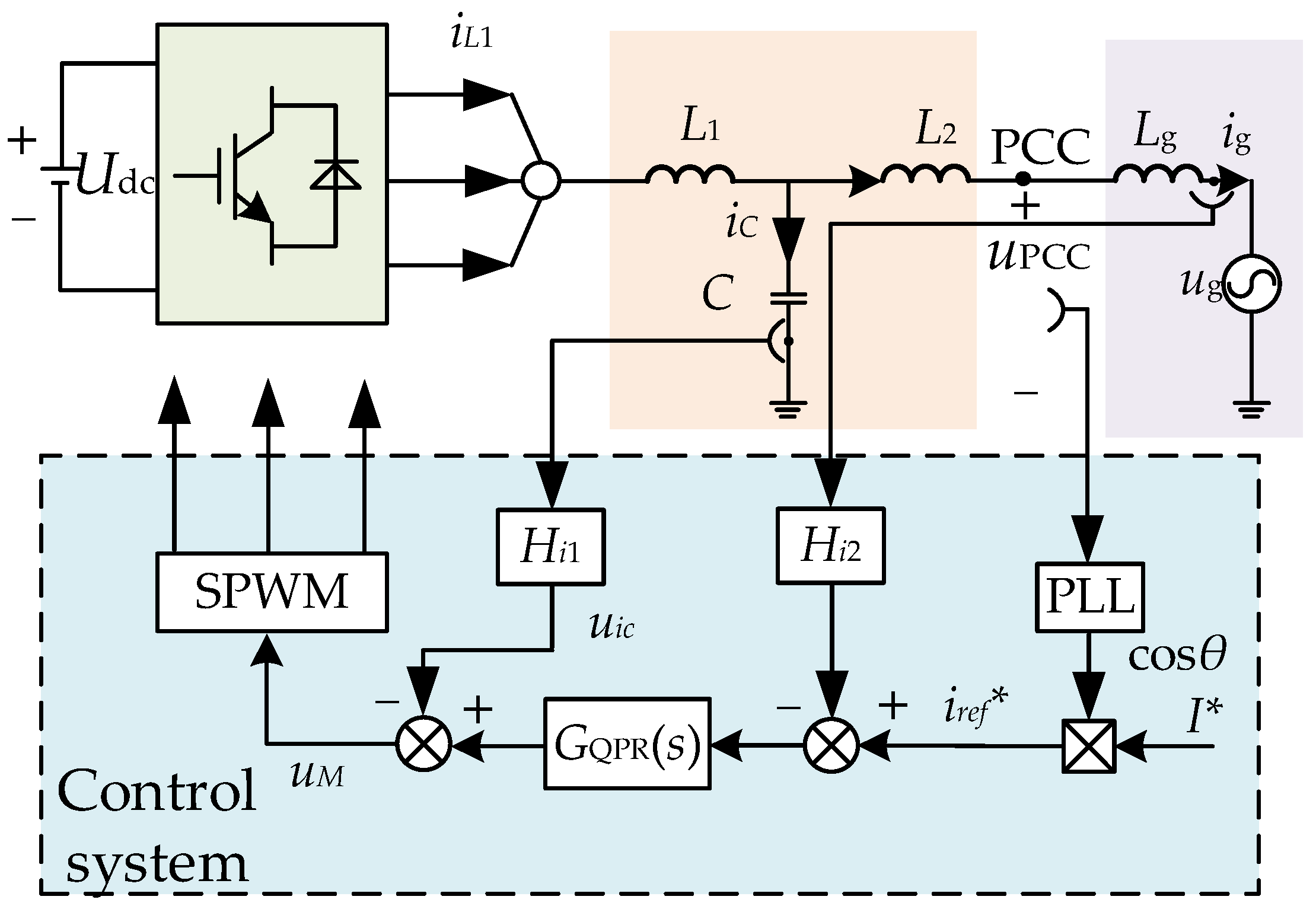
3. Single Inverter Modeling Based on Decomposed Conductance Model

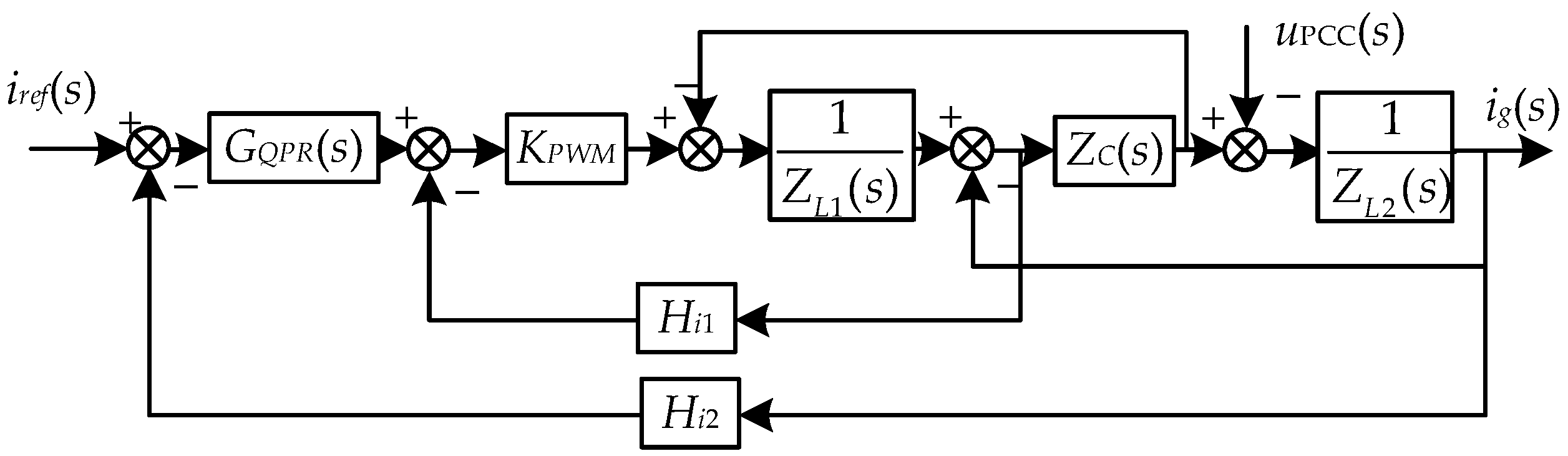
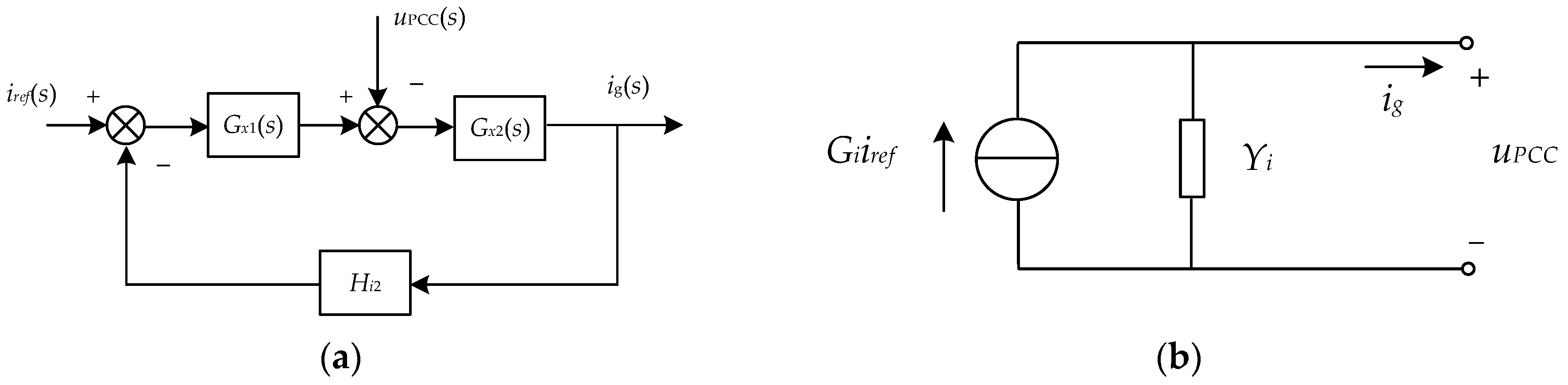
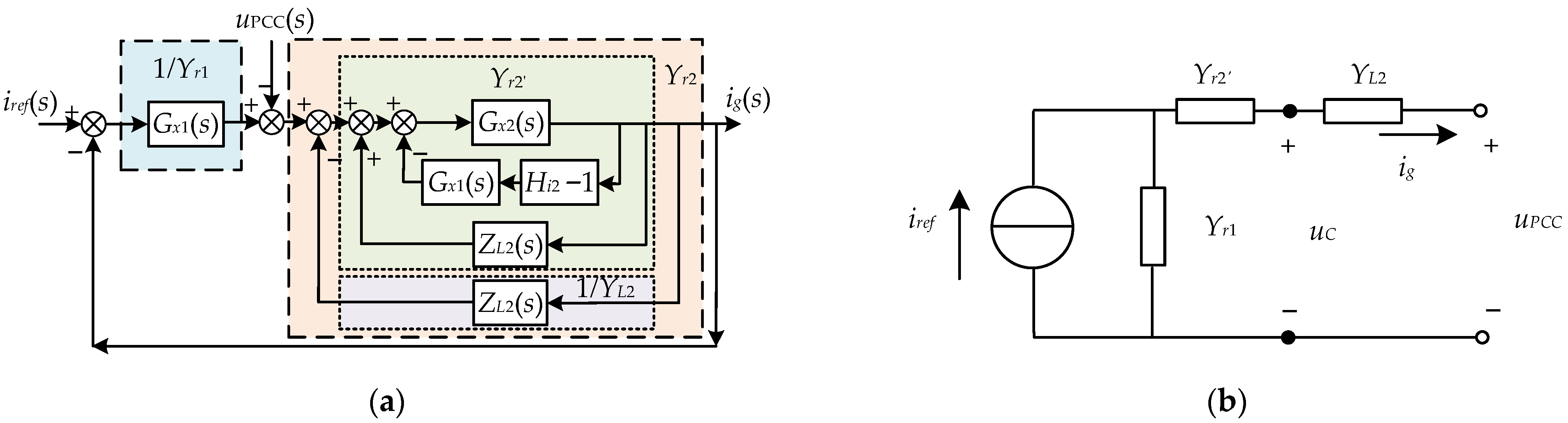
3.1. Norton Equivalent Modeling

The grid-connected structure of the three-phase inverter is shown in Figure 1. The inverter is connected to the power grid through the point of common coupling (PCC). The parameters in Figure 1 are explained as follows: iL is the inverter-side output current, iC is the filter capacitor current, ig is the grid-connected current, and ug is the grid voltage. L1 is the filter inverter-side inductance, L2 is the filter grid-side inductance, C is the filter capacitor, and ZL1(s), ZL2(s), and ZC(s) are their corresponding transfer functions. Lg is the power grid-side reactance in Equation (7).
Z L 1 ( s ) = s L 1 , Z C ( s ) = 1 / ( s C ) , Z L 1 ( s ) = s L 2
The control mathematical model of the inverter is shown in Figure 2. From the Bode diagram of the open-loop transfer function using damping control and undamped control in Figure 3, it can be seen that the damping control has a higher stability margin. To avoid the analysis error caused by the phase-locked loop [21], the control with αβ coordinate system is used, and the active damping control with capacitor current feedback is used to increase the system damping [24]. Where KPWM is the inverter equivalent link, Hi1 is the capacitor current feedback coefficient, and Hi2 is the grid-connected current feedback coefficient.
G Q P R ( s ) = k p + k r ω i s s 2 + 2 ω i s + ω 0 2
The quasi-proportional resonance controller GQPR(s) is used as the current loop modulator in Equation (8), in order to have a better tracking effect of the AC current in αβ coordinate system.
The establishment of the Norton Equivalence Model is shown in Figure 4. To better analyze the system, the control mathematical model of the inverter is equivalently transformed based on Mason’s formula. Gx1(s) and Gx2(s) are the transformed equivalent links in Figure 4a.
G x 1 ( s ) = K P W M G Q P R ( s ) Z C ( s ) Z L 1 ( s ) + Z C ( s ) + H i 1 K P W M
G x 2 ( s ) = Z L 1 ( s ) + Z C ( s ) + H i 1 K P W M { Z L 1 ( s ) Z L 2 ( s ) + H i 1 K P W M Z L 2 ( s ) + [ Z L 1 ( s ) + Z L 2 ( s ) ] Z C ( s ) }
The inverter Norton two-port equivalent model is derived as shown in Figure 4b, where the controlled excitation current source Gi(s)iref(s) is connected in parallel with the conductance Yi(s) to the PCC and then to the power grid, and there are:
i g ( s ) = G i ( s ) i r e f ( s ) Y i ( s ) u P C C ( s )
G i ( s ) = K P W M G Q P R ( s ) A ( s )
Y i ( s ) = s 2 L 1 C + s C H i 1 K P W M + 1 A ( s )
A ( s ) = s 3 L 1 L 2 C + s 2 L 2 C H i 1 K P W M + s ( L 1 + L 2 ) + H i 2 K P W M G Q P R ( s )

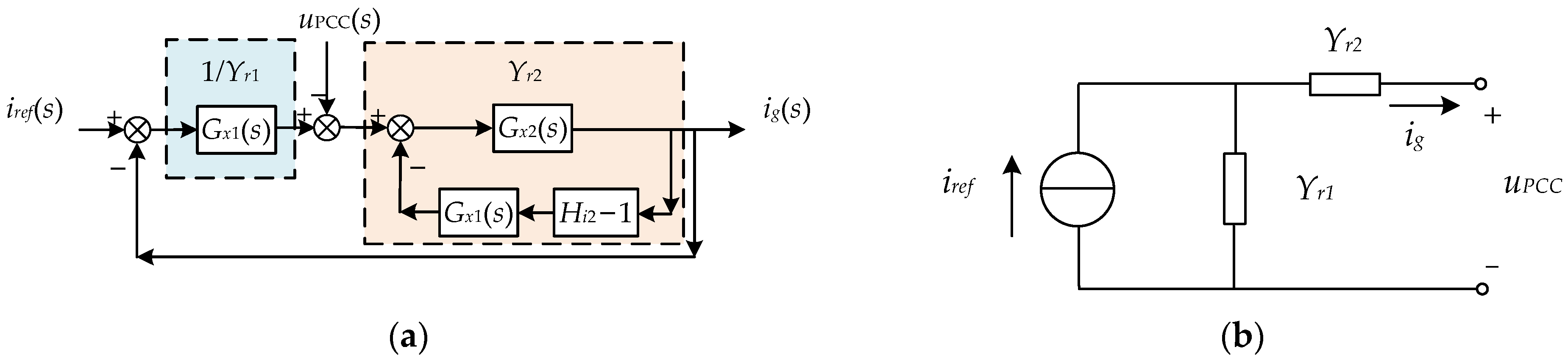
3.2. Decomposition Conductance Modeling

The excitation source iref is equated to the input quantity in the control in order to facilitate the analysis of the effect of iref on the inverter’s grid-connected output current [25]. The control structure of Figure 3 is adjusted by dividing the conductance [18] to separate the antecedent coefficients of iref in the preliminary Norton circuit in Figure 5a, and the two-port equivalent model under double-decomposition conductance is derived based on the divided control structure with Yr1 and Yr2 in Equation (15) as the first and second decomposition conductance, respectively, in Figure 5b.
{ Y r 1 = 1 G x 1 ( s ) = s 2 L 1 C + s C H i 1 K P W M + 1 K P W M G Q P R ( s ) Y r 2 = G x 2 ( s ) 1 + G x 1 ( s ) G x 2 ( s ) ( H i 2 1 ) = s 2 L 1 C + s C H i 1 K P W M + 1 [ s 3 L 1 L 2 C + s 2 L 2 C H i 1 K P W M + s ( L 1 + L 2 ) + ( H i 2 1 ) K P W M G Q P R ( s ) ]
Although the above adjustment can achieve the desired analytical effect, the first and second decomposed derivatives are only equivalent transformations of the control and have no practical physical meaning. Yr2 can be further decomposed into YL2 and Yr2′ in Equation (16), where Zr2, ZL2, and Zr2′ are the reciprocals of Yr2, YL2, and Yr2′, respectively.
Z r 2 = 1 Y r 2 = [ s 3 L 1 L 2 C + s 2 L 2 C H i 1 K P W M + s ( L 1 + L 2 ) + ( H i 2 1 ) K P W M G Q P R ( s ) ] s 2 L 1 C + s C H i 1 K P W M + 1 = s L 2 + s L 1 + ( H i 2 1 ) K P W M G Q P R ( s ) s 2 L 1 C + s C H i 1 K P W M + 1 = Z L 2 + Z r 2 = 1 Y L 2 + 1 Y r 2
The further divided control structure and the two-port equivalent model are shown in Figure 6a,b. Yr1, Yr2′, and YL2 are the first, second, and third decomposed conductors, respectively, and the middle node of conductors Yr2′ and YL2 is the midpoint of the LCL filter. The midpoint voltage corresponds to the voltage uC of the filter capacitor, so that the model has a clear physical meaning, and the multi-inverter system model will be established based on this proposed decomposed conductance model for subsequent analysis and verification.

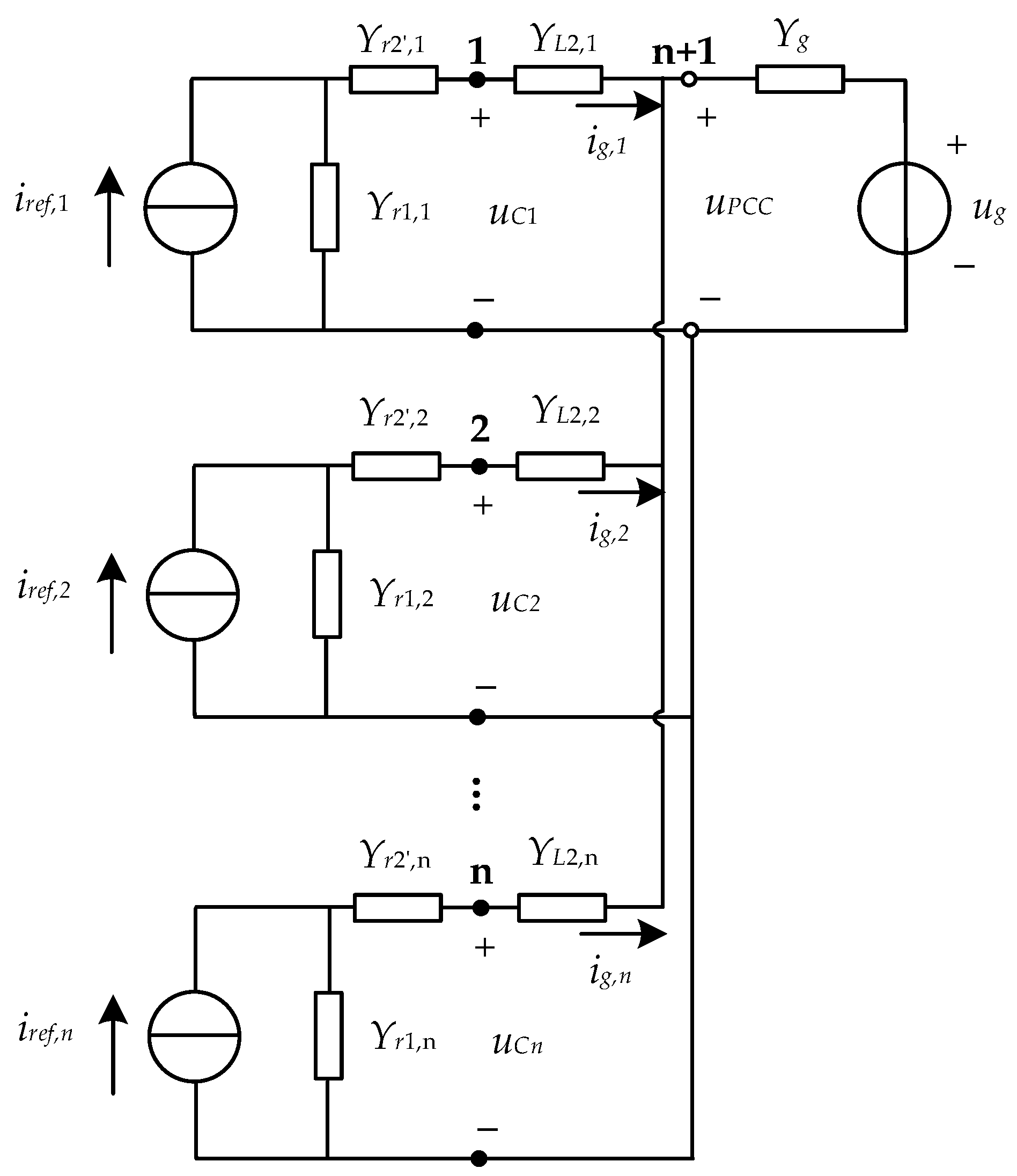
4. Multi-Inverter System Modeling Based on a Decomposed Conductance Model

An equivalent model of the multi-inverter grid-connected system is established, as shown in Figure 7, based on the above two-port equivalent model under the triple decomposition conductance of the single inverter with the power grid side impedance consideration. Clusters of inverters with the number of n are connected to the power grid through PCC, and the grid impedance is expressed by the pure inductive conductance Yg.
The nodes are set in sequence for n inverters, which are numbered, and PCC is numbered n + 1 in Figure 7. The node derivative matrix of the system satisfies the following node voltage equation, as shown in Equation (17).
[ Y 11 0 0 Y 1 ( n + 1 ) 0 Y 22 0 Y 2 ( n + 1 ) 0 0 Y n n Y n ( n + 1 ) Y ( n + 1 ) 1 Y ( n + 1 ) 2 Y ( n + 1 ) n Y ( n + 1 ) ( n + 1 ) ] [ U 1 U 2 U n U P C C ] = [ M 1 i r e f , 1 M 2 i r e f , 2 M 3 i r e f , 2 U g Y g ]
where the matrix elements of the mth inverter satisfy Equation (18).
{ Y m m = Y r 1 , m | | Y r 2 , m + Y L 2 , m   Y m ( n + 1 ) = Y ( n + 1 ) m = Y L 2 , m     Y ( n + 1 ) ( n + 1 ) = Y g + i = 1 n Y L 2 , i M m = Y r 1 , m | | Y r 2 , m / Y r 1 , m
Combining the nodal voltage matrix equation and Kirchhoff’s law, the mth inverter grid-connected current command is derived as shown in Equation (19).
i g , m = Y L 2 , m ( U m U P C C )
The mth node voltage equation is obtained from the node voltage matrix in Equation (20).
Y m m U m + Y m ( n + 1 ) U P C C = M m I r e f , m
Combining with Equation (11), the expression for the grid-connected current of the mth inverter is derived as shown in Equations (21)–(24).
i g , m = R m ( s ) i r e f , m ( s ) k = 1 , k m n P m , k ( s ) i r e f , k ( s ) S g m ( s ) u g ( s )
{ R m ( s ) = Y t e m p , m Y r 1 , m · Y g + i = 1 , i m n Y L 2 , i | | Y e q , i Y g + i = 1 n Y L 2 , i | | Y e q , i P m , k ( s ) = Y t e m p , m Y L 2 , k | | Y e q , k / Y r 1 , k Y g + i = 1 n Y L 2 , i | | Y e q , i , k [ 1 , n ] , k Z , k m S g m ( s ) = Y t e m p , m Y g ( s ) Y g + i = 1 n Y L 2 , i | | Y e q , i
Y t e m p , m = Y e q , m | | Y L 2 , m = Y L 2 , m · Y r 1 , m | | Y r 2 , m Y r 1 , m | | Y r 2 , m + Y L 2 , m
Y e q , m = Y r 1 , m | | Y r 2 , m
Yeq.m is characterized by the equivalent conductance of node m, (m = 1,..., n) on the left side, and Ytemp,m is characterized by the sum conductance of the impedances (equivalent impedance on the left side and impedance of the grid-side filter inductor to the PCC on the right side) on both sides of node m, which is the midpoint of the filter. It can be seen that in a multi-inverter grid-connected system, the grid-connected current of the inverter is affected by its own current command Rm(s), the coupling command Pm,k(s) with other inverters, and the power grid voltage disturbance command Sgm(s). It can be seen that all three command effects are present if grid impedance exists. The resonance of the system is analyzed by the amplitude and frequency response characteristics of each command.

5. Resonant Modal Analysis of a Multi-Inverter Grid-Connected System

The modal analysis method is more convenient than the traditional resonance analysis, and resonance information such as resonance distribution, resonance participation factor, and component sensitivity can be analyzed more comprehensively through the node derivative matrix.
According to the inverter parameters in Table 1, the grid-connected current transfer function derived above and the resonant mode analysis method are used to further compare and analyze the resonance characteristics of the system, as well as the interaction effects of the system. The detailed steps of the resonant modal analysis of a multi-inverter grid-connected system are shown in Figure 8.

5.1. Variation in the Number of Inverters n

The parameters of the grid-connected inverter are selected in Table 1. Only the number of grid-connected inverters n is changed in the following analysis. The magnitude and frequency response characteristic curves of the three commands—the grid-connected current inverter’s own current command Rm(s), the coupling command Pm,k(s) with other inverters, and the grid voltage disturbance command Sgm(s)—are plotted when n is changed, and the resonant modal analysis of the system is carried out to plot the modal impedance curve.
From Figure 9 and Figure 10, it can be obtained that there is only one resonant dominant mode with one resonant frequency if n = 1; when n ≥ 2, two resonant dominant modes are generated due to the interaction excitation between inverters and between inverters and the power grid, which excite low-frequency resonance and high-frequency resonance, respectively. When the number of inverters n (n ≥ 2) increases, the resonant frequency and peak of the high-frequency resonance generated by the system do not change with the increase in n. The resonant frequency of the low-frequency resonance generated by the system gradually shifts to the lower part with the increase of n, and its amplitude also decreases.
Meanwhile, it can be seen that the characteristics of the inverter’s own current command Rm(s) and the coupling command Pm,k(s) of other inverters contain low-frequency and high-frequency characteristics. While the grid voltage disturbance command Sgm(s) can only reflect the low-frequency characteristics because the interaction between the inverters and the power grid cannot yet excite the high-frequency resonance. The resonance characteristics of both low frequency and high frequency can only be generated by multi-source excitation between inverters. The participation factor in the resonant modal analysis method can well reflect the degree of excitation and contribution of each node to various resonant parts. The participation factor of each node with a different number of inverters is calculated, as shown in Table 2. In the low-frequency resonance part, both the inverter and the grid have excitation to it, and the participation factor shows that the inverter is more excitable than the grid; in the high-frequency resonance part, the inverter mainly excites the high frequency, while the participation factor of PCC to the high-frequency part is always 0, so there is no excitability; as the number of inverters increases, the participation factor of the inverter to the low-frequency part decreases, and the excitability to the low-frequency part decreases, while its participation to the high-frequency part increases, so the inverter is more excitable to the high-frequency part.
In Figure 10, it can be seen that Rm(s) can reflect the other two command characteristics. Therefore, the subsequent section only quantitatively analyzes Rm(s).
In this paper, the multi-inverter system at the same connection point is considered, and the inverters of the same manufacturer with the same model parameters are used to ensure cost. Using the inverter models in Table 1, the frequency domain analysis of the inverter’s own coupling command Rm(s) and the resonant mode analysis of the system node conduction matrix are used to further analyze the degree of influence on the resonance characteristics of the system when the grid impedance, the inverter controller parameters, and the inverter filter parameters are varied.

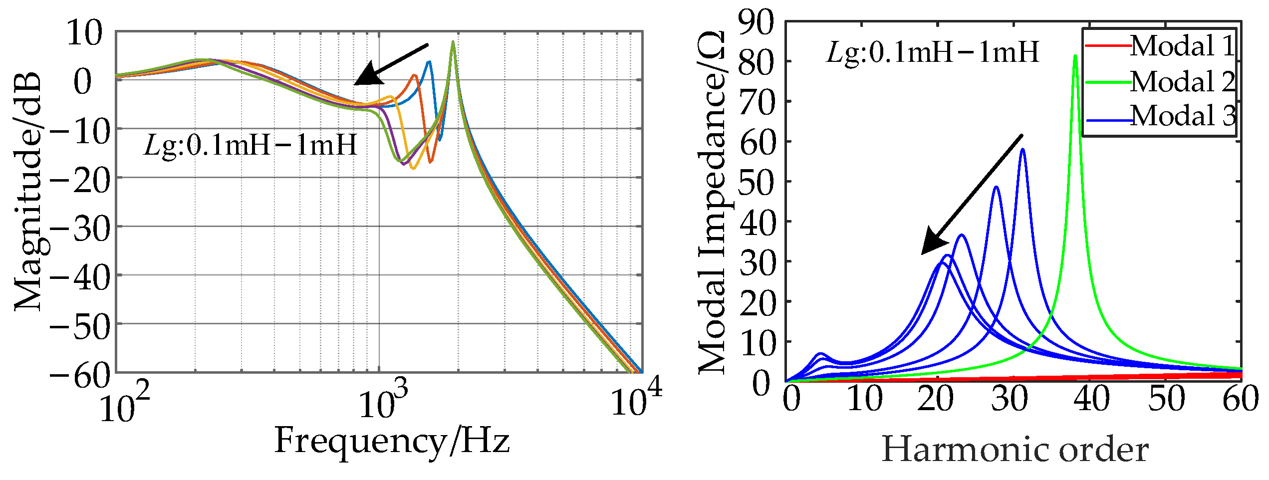
5.2. Impact of Grid Impedance Fluctuations

The system with the number of inverters n = 2 is selected, and the parameters other than the grid impedance are fixed. In Figure 11, the grid impedance Lg is increased from 0.1 mH to 1 mH by ignoring the influence of grid resistance, and it is known from Figure 11 (left) that in the low-frequency resonance part, the modal resonance frequency moves to a lower value with the increase of grid impedance, and the modal impedance, that is, the resonance peak, decreases; in the excitation of high-frequency resonance, the resonance frequency as well as the peak do not change because the grid-side impedance does not participate in the excitation of high-frequency resonance, the frequency domain also verifies the above-mentioned analysis in Figure 11 (right).

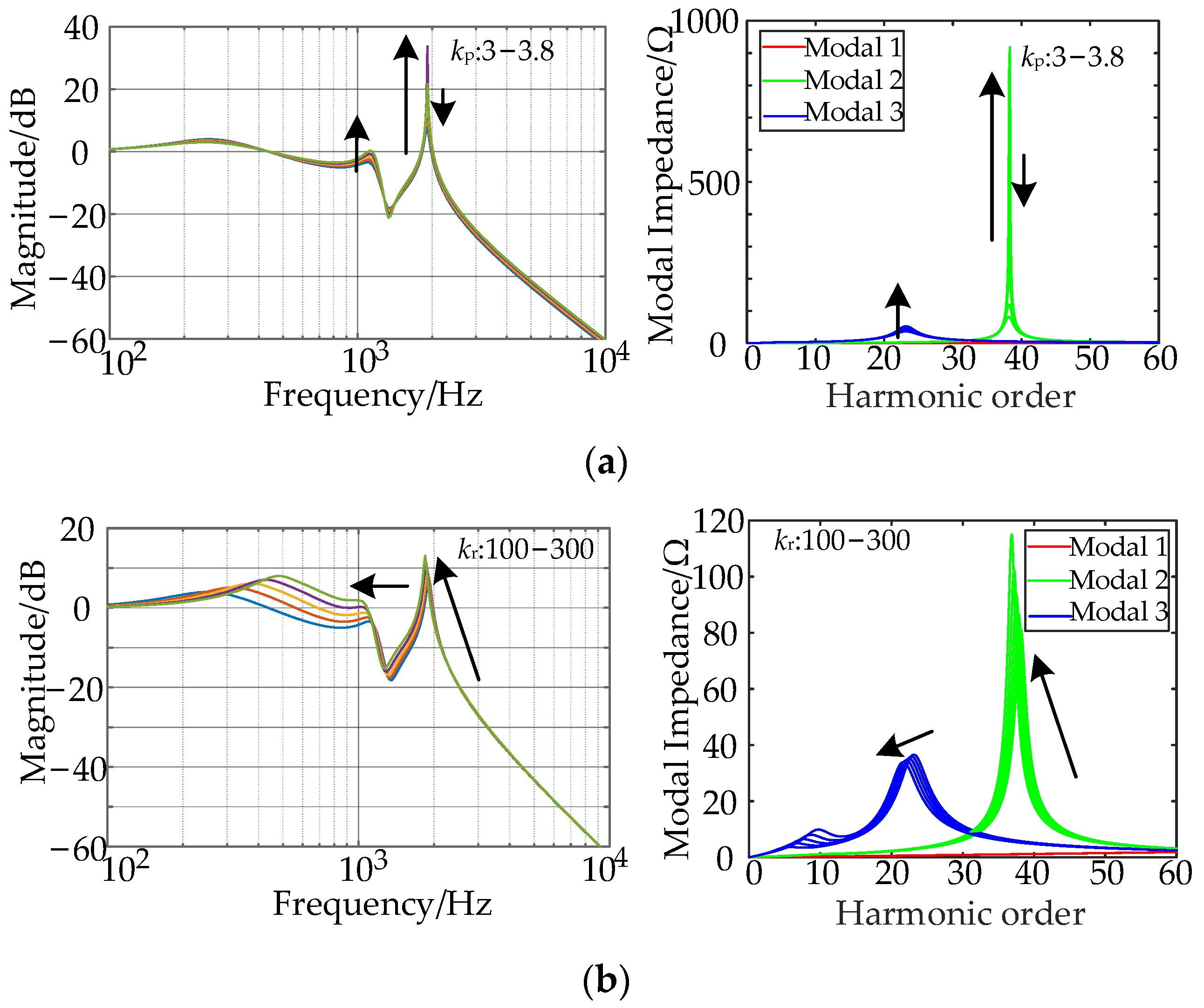
5.3. Impact of Changes in Inverter Control Parameters

The parameters of the quasi-proportional resonance controller are changed to observe its effect on the resonance characteristics of the system. Let kp increase from 3 to 3.8, and it can be found that the resonant frequency of the low-frequency part, as well as the high-frequency part of the mode, does not change, while the resonant mode impedance of the low-frequency part increases with the increase of kp, and the high-frequency part increases in the interval of 3–3.6 and decreases in the interval of 3.6–3.8, and the high-frequency resonance risk is exacerbated, which is also a consistent conclusion in the frequency domain analysis in Figure 12a. From Figure 12b, let kr increase from 100 to 300; at this time, the low-frequency and the high-frequency resonant parts are affected. In the low-frequency resonant part, the mode resonant frequency and mode impedance both move to the low frequency with the increase of kr; in the high-frequency resonant part, the mode resonant frequency decreases and the resonant mode impedance increases with the increase of kr. In addition, the frequency domain analysis also verifies the accuracy of the modal analysis regulation.

5.4. Impact of LCL Filter Parameter Changes

The LCL filter parameters are varied to further observe the effect on the resonant characteristics of the system. By increasing the inverter-side inductor L1 from 0.8 mH to 1.6 mH, it can be seen in Figure 13a that when L1 is increased, the resonant frequency of the low-frequency resonant part shifts to the low frequency, but its corresponding resonant mode impedance increases; the resonant frequency of the high-frequency resonant part decreases; the modal impedance, however, increases. As shown in Figure 13b, when L2 increases, the resonant frequency and resonant mode impedance of the low-frequency part and high-frequency resonant part decrease; when the filter capacitor C increases in Figure 13c, the mode regulation of low-frequency and high-frequency resonance is the same, and its resonant frequency and resonant mode impedance decrease; meanwhile, the frequency domain analysis also verifies the mode analysis regulation when L1 and L2 are changed. When C is changed, although the resonance peak corresponding to the frequency domain analysis has a tendency to increase slightly, its spike state tends to smooth out, and the risk of resonance decreases. The modal impedance reflects the degree of resonance intensity and does not have a practical meaning, so it is consistent with the results of the modal analysis.

5.5. Sensitivity Analysis

The participation factor of the modal analysis method can calculate the excitability and observability of the system nodes for the resonance, while the modal sensitivity calculation can further clarify the influence of the critical components on the resonance characteristics, which can also provide guidance for the suppression of resonance. Define the sensitivity matrix in Equation (25):
S λ = l k t k
For a component connected only in parallel at node i, it takes the form of the conductance expression Yp = G + jB and has a relationship in Equation (26):
λ k Y p = l i k t k i = S λ , i i
The expression of the sensitivity of the eigenvalue and the electron-energy part of the conductance is as shown in Equations (27) and (28).
| λ k | G = d | λ k | d F F G = S r , i j λ r + S i , i j λ i λ r 2 + λ i 2
| λ k | B = d | λ k | d F F B = S r , i j λ i S i , i j λ r λ r 2 + λ i 2
For the component connected in parallel between loops i and j, its impedance expression form is used as Zp = R + jX, and its corresponding sensitivity is solved by converting the form of the conductance to the impedance form, then Equations (29)–(33) can be obtained.
λ k Y p = S λ , i i S λ , j i S λ , i j + S λ , j j
λ k G = μ , λ k B = ν
{ G R = X 2 R 2 R 2 + X 2 , G X = 2 R X R 2 + X 2 B R = 2 R X R 2 + X 2 , B X = R 2 X 2 R 2 + X 2
| λ k | R = | λ k | G G R + | λ k | B B R = μ ( X 2 R 2 ) + 2 ν R X ( R 2 + X 2 ) 2
| λ k | X = | λ k | G G X + | λ k | B B X = μ ( X 2 R 2 ) 2 μ R X ( R 2 + X 2 ) 2
In addition, the sensitivity values reflect the relationship between the components and the eigenvalues in the critical resonant modes. However, the sensitivity values are not comparable to each other, so normalization is done. For the system components α normalized sensitivity is shown in Equation (34).
| λ k | α = | λ k | / λ k α / α = λ k α · α λ k
The sensitivity of the inverter-grid-connected system with n = 2 is calculated as an example. At this time, the resonant frequencies of the system are 23.1 pu and 38.1 pu. The calculation is performed in two cases, one without the decomposed conductance model and one with the decomposed conductance model, and the normalized sensitivity of the system components at each resonant frequency is calculated. As shown in Figure 14a, the sequence numbers 1 to 9 represent the real and imaginary parts of Yg, impedance ZL21~ZL22, and the real and imaginary parts of the left side equivalent conductors of inverter node 1 and inverter node 2, respectively, and the sequence numbers 1 to 13 in Figure 14b represent the real and imaginary parts of Yg, impedance ZL21~ZL22, the real and imaginary parts of conductors Yr1,1~Yr1,2, impedance Zr2′,1~Zr2′,2 real and imaginary parts. A positive normalized value indicates that increasing its value increases the eigenvalue and reduces the modal impedance. A negative normalized value indicates that decreasing its value increases the eigenvalue and decreases the modal impedance. It is obvious that Yg has a negative sensitivity value only at low frequencies, and increasing Lg decreases the modal impedance, which is consistent with the previous analysis, while the high-frequency part, which is mainly influenced by the interaction between inverters, has a greater impact on the high-frequency resonance of its components. The sensitivity analysis without the decomposition method only roughly indicates the global excitability of the inverter, and the low-frequency part is mainly excited by the grid impedance Yg and the equivalent conductance of the inverter, and the high-frequency part is mainly caused by the excitation of ZL2 and the equivalent conductance of the inverter; while the sensitivity analysis of the decomposition of the components using the decomposition conductance model plays a role in refining the analysis, it can be seen that the low-frequency part, except for the excitation effect of Yg, Yr1, Zr2′ all produce a certain excitation effect; in the high-frequency part, all the components except Yg have a certain excitation, among which the component Yr1 and Zr2′ play a major role in the resonance of the high-frequency part, and according to the participation factor, it is also known that the inverter itself is more likely to excite a resonant band with h = 38.1 pu. Therefore, the suppression of Yr1 as well as Yr2′ is more effective for suppressing high-frequency resonance. If Yr1 is suppressed, it is feasible to take corresponding resonance suppression measures between iref(s) and uPCC(s), as the control structure of Yr1 in the inverter can be known; if Yr2′ is suppressed, it is effective to take suppression measures between uPCC(s) and ug(s), as its structure can be known. This gives guidance on resonance suppression, which in turn allows adjustment of critical components that are more involved in reducing the effect of harmonic resonance.

6. Simulation Verification

Based on the simulation platform, two inverter-grid-connected systems are built, and their parameters are referred to in Table 1.
The test currents containing the 23rd and 38th harmonics are injected at the inverter node and the PCC node, and the voltage spectra of UPCC at the PCC node and U1 at the inverter 1 node are observed as shown in Figure 15. It can be seen in Figure 15a that the PCC node cannot yet excite the high-frequency resonance when the 38th harmonic current is injected, and its corresponding participation factor is 0, while the inverter node can well observe that the high-frequency resonance is excited in Figure 15b, which is also consistent with changing the participation factor of the node. When the 23rd harmonic current is injected, both the PCC and the inverter node can excite the low-frequency resonance, and the corresponding participation factors are 0.2270 and 0.3865, respectively, which are consistent with the excitation degree of the low-frequency part in Figure 15.
To verify the correctness of the above modal analysis and spectral analysis results, a typical scenario is selected for simulation to verify the effects on the resonance characteristics of the system when the grid impedance Lg, the inverter-side inductance L1, and the control parameter kr are changed, respectively.
The relationship between the fluctuation of the grid impedance Lg and the resonance characteristics of the system is verified. Fixing other parameters of the system and keeping the number of inverters connected to the grid at two, test currents of the 20th, 32nd, and 38th harmonics are injected into the system at Lg = 0.1 mH and 1 mH, and the corresponding node voltage spectrum changes are shown in Figure 16.
From the spectrum analysis results, it can be seen that when the grid impedance increases, the resonant frequency and harmonic content of the high-frequency part remain unchanged, the resonant frequency of the low-frequency part shifts to the lower part, and the harmonic content at resonance decreases, which is consistent with the results of the modal analysis as well as the frequency domain analysis.
Then, the relationship between the variation of the inverter-side inductor L1 and the resonant characteristics of the system is further verified. In the simulation scenario with two inverters grid-connected, the 22nd, 26th, 38th, and 40th harmonic test currents are injected into the system at L1 = 0.8 mH and 1.6 mH, and the corresponding inverter node voltage spectrum changes are shown in Figure 17a,b.
It can be seen from the spectrum change patterns that when the inductance L1 of the inverter side increases, the resonant frequency of the low-frequency resonant part shifts from the 26th to the 22nd; the resonant frequency of the high-frequency part shifts from the 40th to the 38th; and the resonant frequencies all shift to the low, which is consistent with the results of the modal analysis as well as the frequency domain analysis.
In the previous analysis of the effect of controller parameters, the influence of kp fluctuation on the resonance characteristics of the system was more obvious, so the variation of kp was taken for verification. In the simulation scenario with two inverters grid-connected, test currents of the 23rd and 38th harmonics are injected into the system at kp = 3 and 3.8, respectively, and the corresponding inverter node voltage spectrum changes are shown in Figure 18a,b.
It can be seen from the spectrum change patterns that when the inverter current controller parameter kp is increased, the resonant frequencies of the low-frequency resonance and high-frequency parts do not change, and the resonant amplitude of the high-frequency part increases significantly, and the harmonic content increases, which exacerbates the resonance risk, in accordance with the results of the modal analysis as well as the frequency domain analysis.
The reasonableness of the sensitivity analysis is verified in a scenario where two inverters are grid-connected. Taking the high-frequency resonance part as an example, the analytical structure in the previous section shows that taking resonance suppression measures between iref(s) and uPCC(s) is effective; therefore, this part uses PCC voltage feedforward as shown in Figure 19 to suppress the system resonance. It should be noted in particular that resonance suppression by means of PCC voltage feedforward has been used in [26], but the innovative focus of this paper is not to propose a new suppression method but to quantify the degree of contribution of the system components to resonance by means of sensitivity analysis so that the key components of resonance can be identified for effective resonance suppression. After calculation and testing, Gf = 0.2 is used in the simulation, and the detailed procedure is not repeated.
In Figure 20, the simulation result shows that when the 23rd and 38th harmonic currents are injected at the grid side, the comparison of harmonic voltage amplitudes before and after the inverter adopts the suppression strategy shows that the 23rd harmonic voltage decreases from 1.66 V to 1.41 V and the 38th harmonic voltage decreases from 7.04 V to 5.04 V. The harmonic voltage amplitude is reduced after adopting the suppression strategy, and the effect on high-frequency resonance is more obvious, which verifies the effect from the perspective of the feasibility of suppression from the perspective of sensitivity analysis.

7. Conclusions

The multi-inverter grid-connected system has the characteristics of high order and strong coupling, and the resonance problem generated by it has been widely discussed. In this paper, for the multi-inverter grid-connected system, first the traditional Norton’s equivalent model is improved, and then a multi-inverter grid-connected equivalent model based on the decomposition conductivity model is proposed. Secondly, the resonance characteristics of the system are studied by combining the frequency domain analysis method, the modal analysis method, and sensitivity analysis. Finally, the accuracy of the analysis is verified by simulation, and the following conclusions are drawn.
  • The modal analysis method is easier to calculate than the frequency domain analysis method, which can reflect the resonance information of the multi-inverter system well and can better reflect the observability and excitable degree of resonance of each node of the system.
  • The harmonic resonance of the multi-inverter grid-connected system is affected by the interaction between the inverter and the grid. When the grid impedance is taken into account, two kinds of resonance bands, low-frequency and high-frequency, are generated with the increase of the inverter, and the fluctuation of the grid impedance Lg only affects the low-frequency resonance, while the high-frequency resonance is not affected by it, so the interaction between the grid and the inverter only affects the low-frequency resonance.
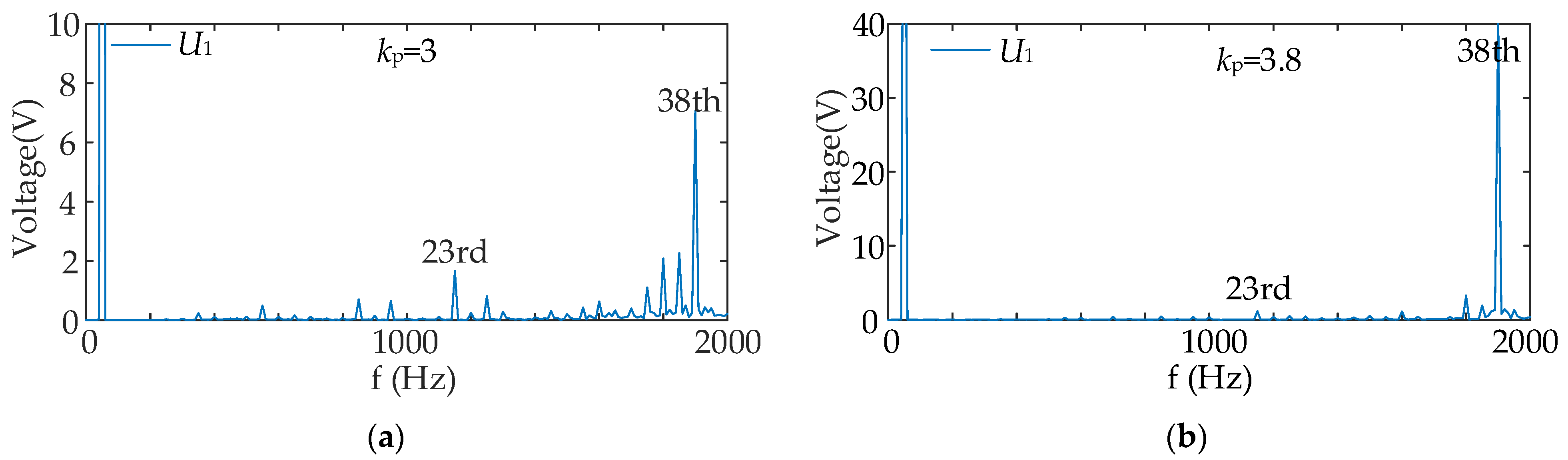
  • The inverter LCL filter parameters and controller parameter fluctuations will have an impact on the low-frequency and high-frequency resonance, where the LCL filter parameter fluctuations have a more significant impact on the resonance. In addition, kp has a more pronounced effect on the high-frequency resonant part.
  • The multi-inverter grid-connected equivalent model based on the decomposition conductance model can refine the influence of each equivalent control link of the inverter on the resonance characteristics of the system through sensitivity analysis and quantify the contribution of the decomposition conductance, in which the first decomposition conductor Yr1 and the second decomposition conductor Yr2′ contribute to the high-frequency resonance to a greater extent.
In this paper, the proposed decomposed conductance model can further quantify the contribution degree of each equivalent control link of the inverter to each resonance band through the conductance division of the control links of the inverter and provide guidance on the direction of resonance suppression; subsequently, it is necessary to add nonlinear factors to be considered together to further carry out relevant research on global resonance suppression measures. In addition, studies on dynamic losses, power losses, and the energy efficiency of converters are also required for further work.

Author Contributions

Conceptualization, L.C., Y.X. and S.T.; methodology, L.C. and Y.X.; software, L.C. and T.W.; validation, L.C., T.W. and S.S.; formal analysis, L.C. and S.T.; investigation, L.C. and Y.X.; resources, Y.X. and S.S.; data curation, Y.X. and S.S.; writing—original draft preparation, L.C. and Y.X.; writing—review and editing, L.C. and Y.X. All authors have read and agreed to the published version of the manuscript.

Funding

This research received no external funding.

Acknowledgments

We appreciate our reviewers and editors for their precious time.

Conflicts of Interest

The authors declare no conflict of interest.

References

  1. Sun, J.; Wu, T.; Ren, J.; Li, M.; Jiang, H. Control and research based on improved LADRC in wind power inverter systems. Electronics 2022, 11, 2833. [Google Scholar] [CrossRef]
  2. Hosseinzadeh, N.; Aziz, A.; Mahmud, A.; Gargoom, A.; Rabbani, M. Voltage stability of power systems with renewable-energy inverter-based generators: A Review. Electronics 2021, 8, 115. [Google Scholar] [CrossRef]
  3. Rocabert, J.; Luna, A.; Blaabjerg, F.; Rodríguez, P. Control of power converters in AC microgrids. IEEE Trans. Power Electron. 2012, 27, 4734–4749. [Google Scholar] [CrossRef]
  4. Agorreta, J.L.; Borrega, M.; López, J.; Marroyo, L. Modeling and control of n-paralleled grid-connected inverters with LCL filter coupled due to grid impedance in PV plants. IEEE Trans. Power Electron. 2011, 26, 770–785. [Google Scholar] [CrossRef]
  5. Wang, X.; Blaabjerg, F. Harmonic stability in power electronic-based power systems: Concept, modeling, and analysis. IEEE Trans. Smart Grid 2019, 10, 2858–2870. [Google Scholar] [CrossRef] [Green Version]
  6. Rygg, A.; Molinas, M.; Chen, Z.; Xu, C. A modified sequence-domain impedance definition and its equivalence to the dq-domain impedance definition for the stability analysis of AC power electronic systems. IEEE J. Emerging Sel. Top. Power Electron. 2016, 4, 1383–1396. [Google Scholar] [CrossRef] [Green Version]
  7. Bakhshizadeh, M.K.; Wang, X.; Blaabjerg, F.; Hjerrild, J.; Kocewiak, L.; Bak, C.L.; Hesselbek, B. Couplings in phase domain impedance modeling of grid-connected converters. IEEE Trans. Power Electron. 2016, 31, 6792–6796. [Google Scholar]
  8. Qi, Q.; Ghaderi, D.; Guerrero, J.M. Sliding mode controller-based switched-capacitor-based high DC gain and low voltage stress DC-DC boost converter for photovoltaic applications. Int. J. Electr. Power Energy Syst. 2021, 125, 106496. [Google Scholar] [CrossRef]
  9. Bulut, K.; Ertekin, D. A novel switched-capacitor and fuzzy logic-based quadratic boost converter with mitigated voltage stress, applicable for DC micro-grid. Electron. Eng. 2022, 104, 4391–4413. [Google Scholar]
  10. Ghaderi, D.; Bayrak, G.; Guerrero, J.M. Grid code compatibility and real-time performance analysis of an efficient inverter topology for PV-based microgrid applications. Int. J. Electr. Power Energy Syst. 2021, 128, 106712. [Google Scholar] [CrossRef]
  11. Sun, J. Impedance-based stability criterion for grid-connected inverters. IEEE Trans. Power Electron. 2011, 26, 3075–3078. [Google Scholar] [CrossRef]
  12. Wang, X.; Blaabjerg, F.; Liserre, M.; Chen, Z.; He, J.; Li, Y. An Active Damper for stabilizing power-electronics-based AC systems. IEEE Trans. Power Electron. 2014, 29, 3318–3329. [Google Scholar] [CrossRef]
  13. Cao, W.; Ma, Y.; Wang, F. Sequence-impedance-based harmonic stability analysis and controller parameter design of three-phase inverter-based multibus AC power systems. IEEE Trans. Power Electron. 2017, 32, 7674–7693. [Google Scholar] [CrossRef]
  14. Wen, B.; Boroyevich, D.; Burgos, R.; Mattavelli, P.; Shen, Z. Inverse Nyquist stability criterion for grid-tied inverters. IEEE Trans. Power Electron. 2017, 32, 1548–1556. [Google Scholar] [CrossRef]
  15. Liu, F.; Zhang, Z.; Ma, M.; Wang, M.; Deng, J.; Zhang, J.; Zhan, M. LCL Filter design method based on stability region and harmonic interaction for grid-connected inverters in weak grid. Proc. CSEE 2019, 39, 4231–4242. [Google Scholar]
  16. Nie, C.; Lei, W.; Wang, Y.; Wang, H.; Feng, G. Resonance analysis of multi-paralleled converter systems and research on optimal virtual resistor damping methods. Proc. CSEE 2017, 37, 1467–1478. [Google Scholar]
  17. Liao, S.; Chen, Y.; Wu, W.; Wang, L.; Xu, Q. Closed-loop interconnected model of multi-inverter-paralleled system and its application to impact assessment of interactions on damping characteristics. IEEE Trans. Smart Grid 2023, 14, 41–53. [Google Scholar] [CrossRef]
  18. Qin, B.; Xu, Y.; Yuan, C.; Jia, J. A Unified method of frequency oscillation characteristic analysis for multi-VSG grid-connected system. IEEE Trans. Power Deliv. 2022, 37, 279–289. [Google Scholar] [CrossRef]
  19. Liu, Q.; Liu, F.; Zou, R.; Li, Y. Harmonic resonance characteristic of large-scale PV plant: Modelling, Analysis, and Engineering Case. IEEE Trans. Power Deliv. 2022, 37, 2359–2368. [Google Scholar] [CrossRef]
  20. Xu, W.; Huang, Z.; Cui, Y.; Wang, H. Harmonic resonance mode analysis. IEEE Trans. Power Deliv. 2005, 20, 1182–1190. [Google Scholar] [CrossRef]
  21. Hong, L.; Shu, W.; Wang, J.; Mian, R. Harmonic resonance investigation of a multi-inverter grid-connected system using resonance modal analysis. IEEE Trans. Power Deliv. 2019, 34, 63–72. [Google Scholar] [CrossRef]
  22. Wu, J.; Chen, T.; Han, W.; Zhao, J.; Li, B.; Xu, D. Modal analysis of resonance and stable domain calculation of active damping in multi-inverter grid-connected systems. J. Power Electron. 2018, 18, 185–194. [Google Scholar]
  23. Liu, Y.; Shuai, Z.; Li, Y.; Cheng, Y.; Shen, Z. Harmonic resonance modal analysis of multi-inverter grid-connected systems. Proc. CSEE 2017, 37, 4156–4164+4295. [Google Scholar]
  24. Pan, D.; Ruan, X.; Bao, C.; Li, W.; Wang, X. Capacitor-current-feedback active damping with reduced computation delay for improving robustness of LCL-type grid-connected inverter. IEEE Trans. Power Electron. 2014, 29, 3414–3427. [Google Scholar] [CrossRef]
  25. Yu, C.; Zhang, X.; Liu, F.; Li, F.; Xu, H.; Cao, R.; Ni, H. Modeling and resonance analysis of multiparallel inverters system under asynchronous carriers conditions. IEEE Trans. Power Electron. 2017, 32, 3192–3205. [Google Scholar] [CrossRef]
  26. Wang, X.; Ruan, X.; Liu, S.; Tse, C.K. Full feedforward of grid voltage for grid-connected inverter with LCL filter to suppress current distortion due to grid voltage harmonics. IEEE Trans. Power Electron. 2010, 25, 3119–3127. [Google Scholar] [CrossRef]
Figure 1. A structure diagram of an LCL inverter.
Electronics 12 01251 g001
Figure 2. Mathematical model of capacitive current feedback active damping control method.
Electronics 12 01251 g002
Figure 3. The Bode diagram of the open-loop transfer function using damping control and conventional undamped control.
Electronics 12 01251 g003
Figure 4. The establishment of the Norton Equivalence Model: (a) Equivalent transformation of the mathematical model; (b) The Norton two-port equivalent model.
Electronics 12 01251 g004
Figure 5. The establishment of the double-decomposed conductance model: (a) the double-decomposed conductance small signal model; (b) the two-port equivalent model under the double-decomposed conductance.
Electronics 12 01251 g005
Figure 6. The establishment of the triple decomposed conductance model: (a) The triple decomposition conductance small signal model; (b) The two-port equivalent model under triple decomposition conductance.
Electronics 12 01251 g006
Figure 7. The equivalent model of a multi-inverter grid-connected system.
Electronics 12 01251 g007
Figure 8. The specific process of resonant mode analysis.
Electronics 12 01251 g008
Figure 9. The modal impedance curve when n is changed: (a) n = 1; (b) n = 2; (c) n = 3; (d) n = 4.
Electronics 12 01251 g009
Figure 10. The characteristics of the amplitude-frequency response of each command of the inverter’s grid-connected current.
Electronics 12 01251 g010
Figure 11. The resonance characteristic curve changes when Lg is changed.
Electronics 12 01251 g011
Figure 12. The resonance characteristics curve when the inverter controller parameters are changed: (a) kp; (b) kr.
Electronics 12 01251 g012
Figure 13. The resonance characteristics curve when the LCL parameters are changed: (a) L1; (b) L2; (c) C.
Electronics 12 01251 g013
Figure 14. The results of the sensitivity analysis comparison are: (a) the sensitivity without the decomposed conductance model; (b) the sensitivity using the decomposed conductance model.
Electronics 12 01251 g014
Figure 15. The node voltage spectrum at n = 2: (a) UPCC; (b) U1.
Electronics 12 01251 g015
Figure 16. The node voltage spectrum when Lg is varied: (a) Lg = 0.1 mH; (b) Lg = 1 mH.
Electronics 12 01251 g016
Figure 17. The node voltage spectrum when L1 is changed: (a) L1 = 0.8 mH; (b) L1 = 1.6 mH.
Electronics 12 01251 g017
Figure 18. The node voltage spectrum when L1 is changed: (a) kp = 3; (b) kp = 3.8.
Electronics 12 01251 g018
Figure 19. The resonance suppression strategy with PCC voltage feedforward.
Electronics 12 01251 g019
Figure 20. The comparison of the harmonic voltage of Inverter 1 before and after adopting the resonance suppression strategy.
Electronics 12 01251 g020
Table 1. The parameters of the grid-connected inverter.
ParametersSymbolValue
Power grid voltageUg/V220
Power grid impedanceLg/mH0.5
Inverter-side inductorL1/mH1.2
Grid-side inductanceL2/mH0.3
Filter CapacitorC/μF28
Quasi-proportional resonance controller parameterskp3
ki100
ωi/rad·s−15
Capacitive current feedback coefficientHi13
Grid-connected current feedback coefficientHi21
Table 2. The participation factor of each node when the number of grid-connected inverters is changed.
nFrequency/puNode
12345
223.10.38650.38650.2270
38.10.50000.50000
321.50.27110.27110.27110.1867
38.10.66670.66670.66670
420.60.21060.21060.21060.21060.1578
38.10.74800.74970.74140.74140
Disclaimer/Publisher’s Note: The statements, opinions and data contained in all publications are solely those of the individual author(s) and contributor(s) and not of MDPI and/or the editor(s). MDPI and/or the editor(s) disclaim responsibility for any injury to people or property resulting from any ideas, methods, instructions or products referred to in the content.

