A Prognosis Technique Based on Improved GWO-NMPC to Improve the Trajectory Tracking Control System Reliability of Unmanned Underwater Vehicles

Abstract

The dynamics model of the unmanned underwater vehicle (UUV) system is highly nonlinear, multi-degree-of-freedom, strongly coupled, and time-varying. Its motion control has been a complex problem due to the unknown information about and the uncertainty of the working environment. To improve the performance and reliability of UUV trajectory tracking control, a trajectory tracking method based on nonlinear model predictive control is designed, and an improved gray wolf optimization (IGWO) is proposed for the optimization of nonlinear model predictive control. The convergence factor of IGWO is designed as a nonlinear attenuation function, and the memory function is added to the position update equation to enhance the effect of trajectory tracking control. Through the simulation in the ROS environment, the influence of the convergence factor on the convergence rate of trajectory tracking error and tracking control performance is obtained. By comparing the tracking effects of several groups of reference trajectories, it is shown that the proposed method is universally applicable and effective to the trajectory tracking control of UUV. Compared with traditional gray wolf optimization (GWO), SQP, and other optimization algorithms, the reliability of the proposed method for UUV trajectory tracking control is demonstrated.

1. Introduction

Unmanned underwater vehicles (UUVs) can perform several more complex tasks, including exploration of the marine environment and extraction of underwater resources, as well as military exploration and surveillance missions in particular sea areas [1]. Trajectory tracking control, as one of the critical technologies of UUVs, is an essential prerequisite for accomplishing specific tasks [2]. For this reason, the study of trajectory tracking control for UUVs in marine missions is very important.

Common UUV trajectory tracking control methods for complex and unknown marine environments include PID control, sliding mode control, fuzzy control, adaptive control, predictive control, etc. [3]. Carlos et al. used the proposed two-level nonlinear PID to complete the depth-tracking control of an underwater glider [4]. Adrian et al. proposed a strategy based on the combination of integral sliding mode control technology and a super twist controller, which has achieved good results in the three-dimensional trajectory tracking control of a four-degree-of-freedom underwater vehicle [5]. Yin et al. solved the problem of dynamic trajectory tracking of UUV using the variable fuzzy predictive control method [6]. Compared with these methods, model predictive control (MPC) has an advantage in solving multi-input and multi-output motion control problems with constraints. Its ability to model prediction for the future is an effect that cannot be achieved by traditional control methods [7].

For such a highly nonlinear, multi-degree-of-freedom, strongly coupled, and the time-varying system as UUV, the design of its nonlinear model predictive control (NMPC) is faced with many problems. It is mainly reflected in the fact that, for complex UUV system models, it is easy to have insufficient search ability and unstable accuracy in predicting future states [8]. Due to the severe influence of the underwater environment, the UUV underwater exploration task’s path is often complex, requiring a lot of calculation and time to solve optimization problems [9]. Houska et al. proposed an automatically generated microsecond NMPC real-time iterative algorithm. The algorithm reduces the number of iterations by decreasing the accuracy of the optimization solution at the beginning. However, this has some degree of impact on global optimization performance [10]. Zhang applied a robust linearized MPC to ensure the stability of surface ships in a disturbing environment [11]. Clearly, for highly nonlinear and disturbed UUV control systems, the linearization technique is minimal when the reference trajectory changes substantially, and it is easy to cause a significant overshoot [12,13]. Liu et al. studied an improved NMPC method, using a nonlinear disturbance observer (NDOB) to estimate the environmental disturbance, which enhanced the robustness of the controller. To improve the control performance of USV trajectory tracking, the event-triggering mechanism reduces the calculation speed of NMPC in trajectory tracking control, making it challenging to ensure real-time control [14]. Li et al. used the dynamic real-time optimization (DRTO) formula with closed-loop prediction to coordinate the distributed model predictive controller. It replaces MPC quadratic programming subproblem with an equivalent Karush Kuhn Tucker (KKT) first-order optimality condition, which improves the optimization speed. The control accuracy still needs to be effectively solved [15]. Shen et al. studied NMPC for autonomous underwater vehicle (AUV) trajectory tracking control and proposed an improved continuation/generalized minimum residual (C/GMRES) algorithm on the optimization algorithm [16]. This way, the contradiction between the short sampling period and the high requirement of online calculation can be alleviated. However, the stability of the numerical algorithm in the global optimization process has yet to be well improved, which needs to be further solved. Therefore, an urgent problem needing to be solved is how to make new attempts and improvements to the optimization algorithm of NMPC to alleviate the high requirements for online computing and improve the algorithm’s stability in the optimization process.

The research and development of UUV in the optimization algorithm of NMPC trajectory tracking control are mainly faced with real-time control performance and stability problems [17]. Currently, the heuristic swarm intelligence optimization algorithm is widely used to optimize various industrial sites [18]. Compared with other algorithms, it has a faster convergence speed and can reduce computational work. However, it also needs more stability and can guarantee the optimal solution. Compared with other population intelligence algorithms, GWO has the advantages of fast convergence speed, strong robustness, and high accuracy. Recently, it has been widely used in various optimization strategy problems [19]. However, GWO also has the issues of slow convergence speed and access to falls into local optimal solutions [20]. Many researchers have also proposed many improved GWO algorithms for this purpose. Mittal et al. adjusted the parameters of the convergence factor by using the exponential decay function and proposed an enhanced GWO algorithm to improve the optimization performance of the GWO algorithm [21]. Wen et al. combined the decay function with the logarithmic function and proposed a nonlinear decay convergence factor adjustment based on the particle swarm algorithm method [22,23]. Chu et al. presented adaptive nonlinear model predictive control technology and designed a trajectory tracking controller for AUV. By establishing the RBF neural network prediction model, the adaptive GWO algorithm is used to solve the optimization problem. However, the convergence speed in the optimization process needs to be balanced on the whole, which is easy to make the optimization fall into the local optimum and reduce the control accuracy [24]. Although the above research aims to balance global exploration and local exploitation in the optimization solution process, they overemphasize the ability in one aspect. This causes the decay rate of the convergence factor to be relatively fast or slow in the whole world, which makes it difficult to effectively balance the searchability and convergence rate of the optimization and does not provide the best solution for the decay form of the convergence factor. Therefore, it is necessary to propose new solutions to better balance the global exploration and local exploitation capabilities in GWO. It is essential to improve the real-time performance of nonlinear model predictive control efficiency and ensure the global exploration accuracy of control.

This paper studies the trajectory tracking control method of UUV based on NMPC. Based on the above problems, the contributions made in this paper are summarized as follows:

• The NMPC method is applied to the trajectory tracking control of UUV, and the nonlinear model predictive controller is designed. By predicting the state of the established model at each sampling time point in the future, the tracking effect of the determined trajectory is improved.
• An improved nonlinear convergence factor GWO is proposed and applied to the designed NMPC to improve the optimization performance of the NMPC and ensure the stability of the trajectory tracking control effect.
• The designed NMPC is transplanted in the ROS-based UUV simulation environment. In a simulation environment, the trajectory tracking tests are carried out on different reference trajectories in the built experimental simulation environment to verify the effectiveness of the proposed trajectory tracking method of the UUV.

The main structure of this paper is as follows: The problems studied in this paper are introduced in Section 2, including the kinematic and dynamic models of the underwater vehicle and the trajectory tracking. The design process of the NMPC is described in Section 3. The simulation experiment carried out under the UUV environment is shown in Section 4, including the construction of the test environment and the results of optimization and tracking. The last part synthesizes the consequences related to the simulation experiments and the further work that can be carried out in the future.

2. Problem Description

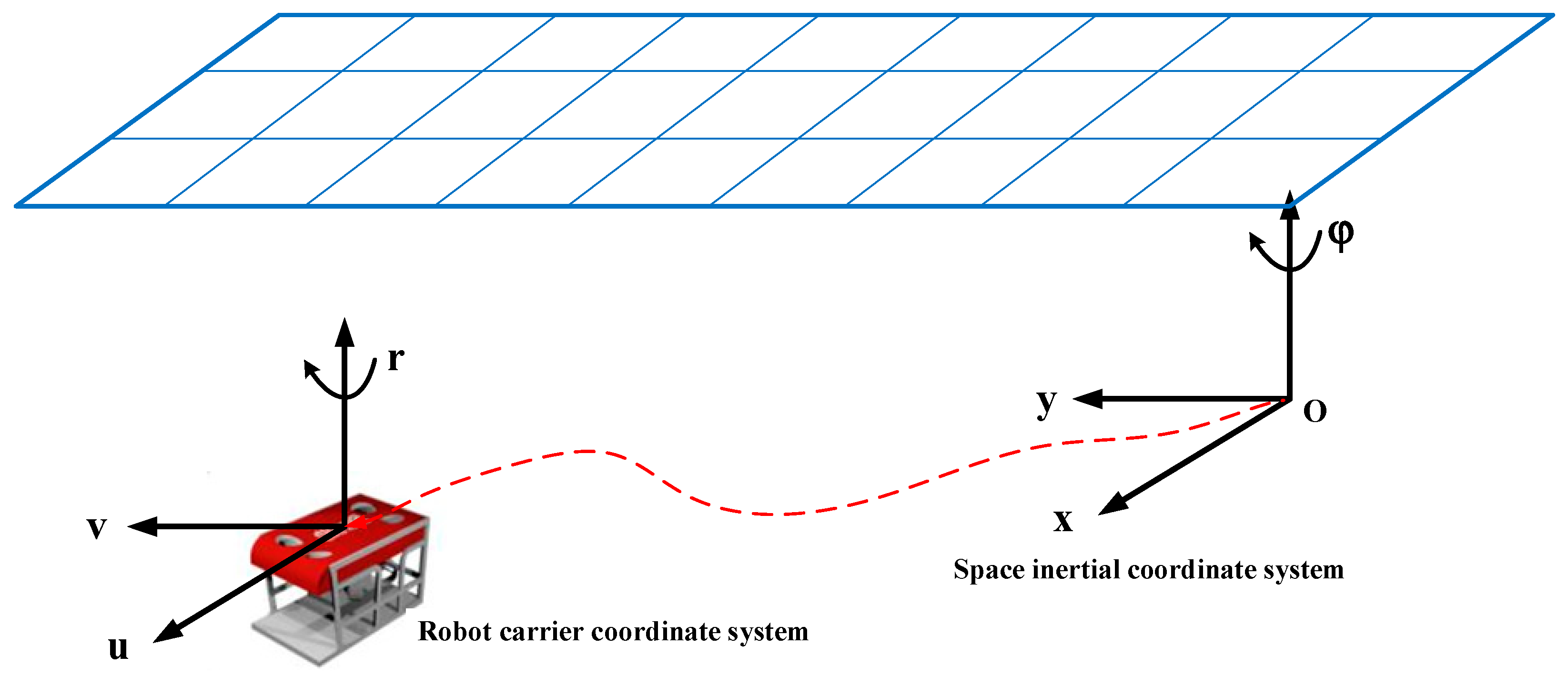
The control objectives of UUV in the motion process include the robot’s position, posture, velocity, and angular velocity [24], involving six degrees of freedom of motion control. These control variables are often artificially decoupled into two types in engineering applications: horizontal plane control and vertical plane control. This paper mainly studies the trajectory tracking of the horizontal plane control; thus, the model is simplified to a three-degree-of-freedom model in the horizontal plane. As shown in Figure 1, the three-degree-of-freedom model of the UUV and its coordinate system are described.

According to the Newton–Euler equations of motion for a rigid body in a fluid [25], the dynamic equations of motion of UUV in the established coordinate system can be derived:

$$M\dot{\mathrm{v}}+C\left(\mathrm{v}\right)\mathrm{v}+D\left(\mathrm{v}\right)\mathrm{v}+g\left(\eta \right)=\tau$$

(1)

where $\eta ={\left[x,y,\phi \right]}^T$ denotes the position and orientation of UUV in an inertial coordinate system. $\nu ={\left[u,v,r\right]}^T$ indicates the velocity of UUV in the moving coordinate system. $\tau ={\left[F_u,F_v,F_r\right]}^T$ denotes the thrust force. $M=diag\left(M_x,M_{y,}{M}_{\psi }\right)$ represents the UUV inertia matrix, including the additional mass. The additional mass represents the additional inertial force generated by the change of fluid velocity around the vehicle. $D\left(\nu \right)=diag\left(X_u,Y_v,N_r\right)+diag\left(D_u\left|u\right|,D_v\left|v\right|,D_r\left|r\right|\right)$ is the damping matrix, the restoring force $g\left(\eta \right)=0$. The Coriolis matrix is expressed as:

$$C\left(\nu \right)=\left[\begin{array}{ccc}0& 0& -M_{y}v\\ 0& 0& M_{x}u\\ M_{y}v& -M_{x}u& 0\end{array}\right]$$

(2)

Expanding the element expression in dynamic Equation (1), we have:

$$\dot{u}=\frac{M_y}{M_x}vr-\frac{X_u}{M_x}u-\frac{D_u}{M_x}u\left|u\right|+\frac{F_u}{M_x}$$

(3)

$$\dot{v}=-\frac{M_x}{M_y}ur-\frac{Y_v}{M_y}v-\frac{D_v}{M_y}v\left|v\right|+\frac{F_v}{M_y}$$

(4)

$$\dot{r}=\frac{M_x-M_y}{M_{\psi }}uv-\frac{N_r}{M_{\psi }}r-\frac{D_r}{M_{\psi }}r\left|r\right|+\frac{F_r}{M_{\psi }}$$

(5)

The kinematics equation of UUV under the established coordinate system can be described as [26]:

$$\dot{\eta }=J\left(\eta \right)\mathrm{v}$$

(6)

According to the conversion relationship between the UUV carrier coordinate system and the inertial coordinate system, the velocity conversion matrix of the UUV three-degree of freedom model in the horizontal plane can be established. The definition is as follows:

$$J\left(\eta \right)=\left[\begin{array}{ccc}cos\phi & -sin\phi & 0\\ sin\phi & cos\phi & 0\\ 0& 0& 1\end{array}\right]$$

(7)

Expanding the element expression of kinematic Equation (5), we have:

$$\dot{x}=u cos\phi -v sin\phi$$

(8)

$$\dot{y}=u sin\phi +v cos\phi$$

(9)

$$\dot{\phi }=r$$

(10)

Binding the dynamic equations and kinematic equations together, the control system model is established as follows:

$$\dot{x}=\left[\begin{array}{c}J\left(\eta \right)v\\ M^{-1}\left(u-Cv-Dv-g\right)\end{array}\right]=f\left(x,\mathsf{\tau }\right)$$

(11)

where $x={\left[x,y,\phi ,u,v,r\right]}^T$, represents the state volume of the UUV. $\mathsf{\tau }={\left[F_u,F_v,F_r\right]}^T$, represents the amount of control over the horizontal motion of the UUV.

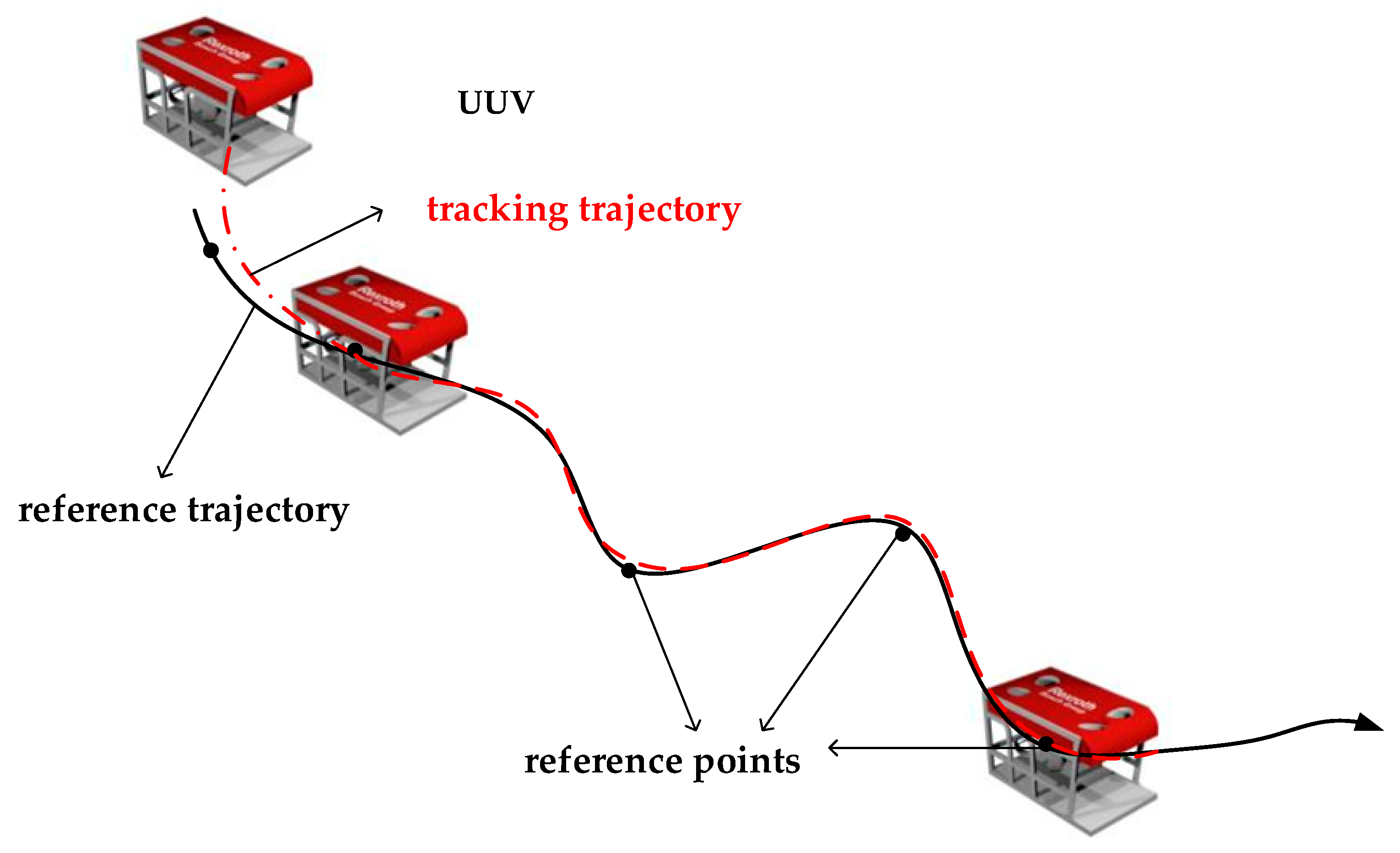
The trajectory tracking process of the UUV studied in this paper is shown in Figure 2 below.

In the inertial coordinate system, the UUV starts from its initial position. A given reference path consisting of N discrete reference points $s_1,s_2,\dots s_N$ should not only meet the physical property constraints of the UUV itself, but also meet the kinematic equations. For which the reference points $s_t={[x_R\left(t\right),y_R\left(t\right)]}^T$, all should satisfy the following differential relation [27,28]:

$${\dot{x}}_R=u_{R}cos{\psi }_R-v_{R}sin{\psi }_R$$

$${\dot{y}}_R=u_{R}sin{\psi }_R+v_{R}cos{\psi }_R$$

(12)

$${\dot{\psi }}_R=r_R$$

where $x_R$, $y_R$ and ${\phi }_R$ indicate the coordinate position and heading angle of the reference point in the space inertial coordinate system, respectively. $u_R$, $v_R$ and $r_R$ represent the linear velocity and angular velocity of the reference point of the robot carrier coordinate system, respectively.

By transforming the solution based on Equation (8), the real-time state quantities can be expressed in terms of position points $x_R$ and $y_R$ in the horizontal plane as:

$$\left\{\begin{array}{c}{\psi }_R=\mathrm{atan}2\left({\dot{y}}_R,{\dot{x}}_R\right)\\ u_R=\sqrt{{\dot{x}}_R^2+{\dot{y}}_R^2}\\ v_R=0\\ r_R=\left({\dot{x}}_R{\ddot{y}}_R-{\dot{y}}_R{\ddot{x}}_R\right)/\left({\dot{x}}_R^2+{\dot{y}}_R^2\right)\end{array}\right.$$

(13)

The function of the NMPC trajectory tracking controller designed in this paper is to solve the corresponding control law for each sampling time, so that the actual state of UUV at each time can track the reference state as much as possible. Considering that UUV is affected by hydrodynamics and hydrodynamic effects in the ROS environment, the controller optimizes the control objective function through improved IGWO. Thus, the current control quantity can be determined, and the control law can be automatically adjusted to change the UUV’s motion state; thus, it can always move on the desired trajectory.

3. Controller Design

In this section, an NMPC controller for trajectory tracking control of UUV is designed, which improves the iterative calculation rate and real-time control by enhancing the traditional optimization algorithm. The control stability and accuracy of the system model are compensated by strengthening the optimal global exploration and local exploitation ability. At the same time, the improved optimization method can realize the controller algorithm’s online parameter adjustment to meet the UUV’s control requirements in the experimental environment to improve the comprehensive control performance of the controller.

3.1. Nonlinear Model Predictive Controller

In the NMPC proposed in this paper, the UUV system model is nonlinear; therefore, the corresponding predictive model is also nonlinear. However, similar to the traditional MPC, its core is to optimize the control variables for each sampling period, starting from the system’s current state. The objective function is optimized through the improved optimization algorithm in the finite prediction time domain to obtain an optimal control law, and the first control quantity of the sequence is applied to the controlled UUV system.

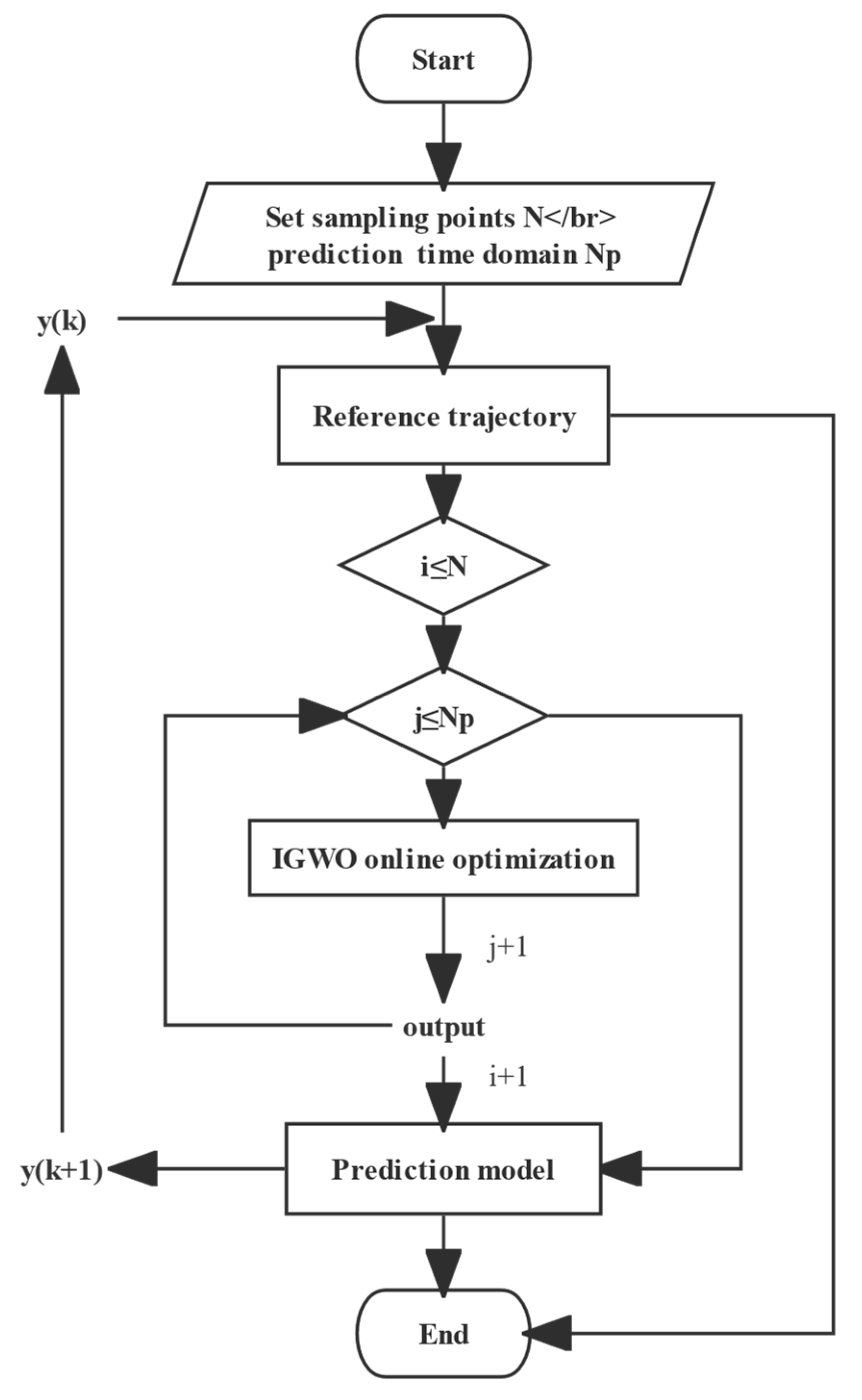
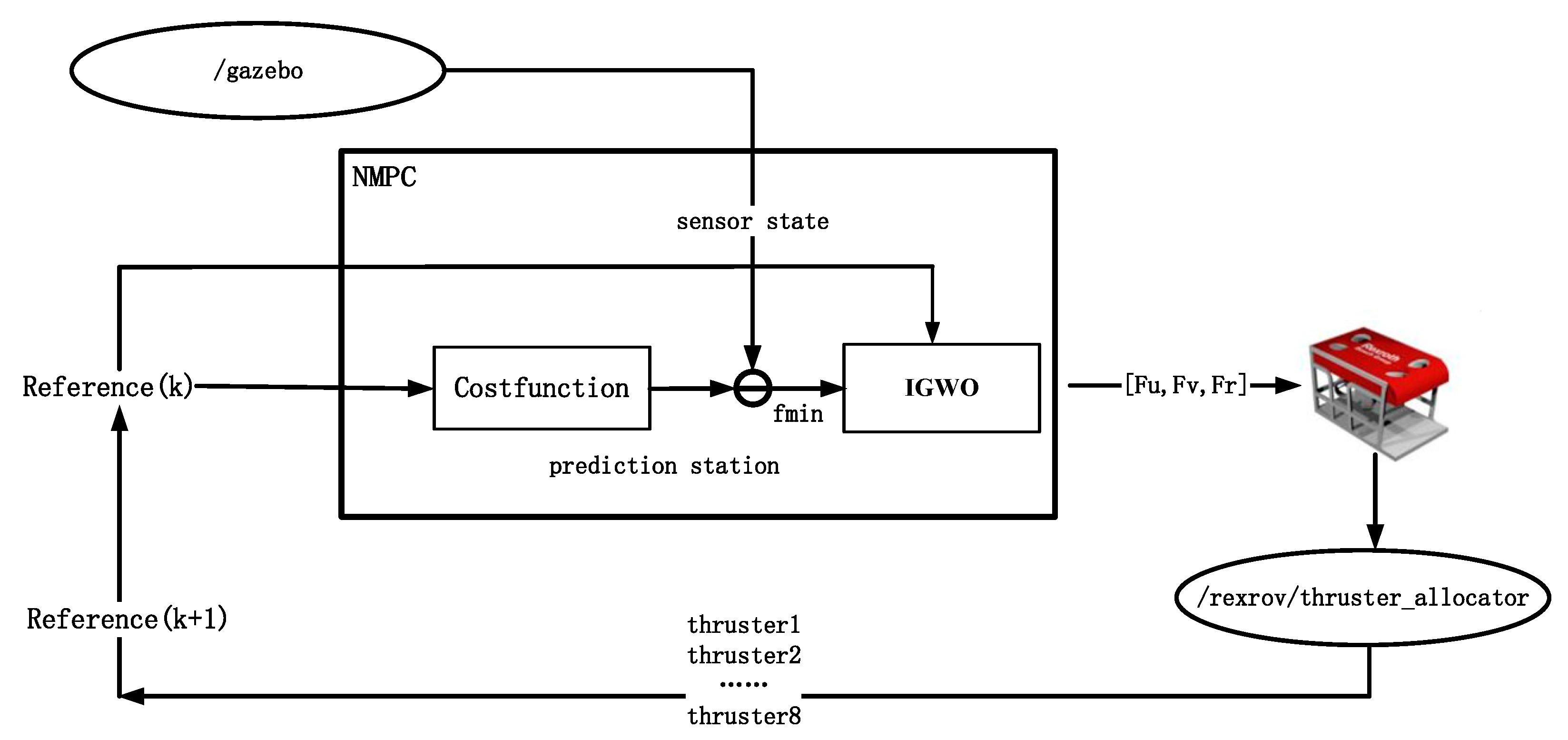
The NMPC framework built in this paper is shown in Figure 3. The process includes the generation of reference trajectory, rolling optimization, model prediction, and introduction of the control law. At each sampling time, the controller performs rolling optimization in a finite time domain for a given reference trajectory to obtain the optimal control output u at the corresponding time. Then, this is applied to the UUV system and the corresponding prediction model to obtain the system’s current output and prediction output, denoted as $P\left(k\right)$ and $P_m\left(k\right)$, respectively. The deviation $e\left(k\right)$ between them is fed back to the objective function of the optimizer through the predictor. On the other hand, the system output $P_p\left(k+1\right)$ acquired through the sensor is taken as the following initial information and transmitted to the optimizer, etc., until the whole process is completed.

The flow chart of the controller proposed in this paper is shown in Figure 4 below:

3.2. Objective Function and Constraints

The corresponding model parameters of the UUV can be obtained through model analysis. Combined with the dynamic model (1), the matrix expansion in the equation is solved to collate the expressions for the linear velocity of the vehicle in each axis direction and the angular velocity of rotation around each axis. Given the robot’s initial position, the velocity vector of three degrees of freedom in the horizontal direction at each time in the prediction time domain is recorded as $\mathbf{y}\left(k\right)$, i.e., $\mathbf{y}\left(k\right)={[u\left(k\right),v\left(k\right),r\left(k\right)]}^T$. It can be expressed as Formula (10):

$$\left\{\begin{array}{l}u\left(k\right)=\left(\frac{F_u\left(k\right)}{M_x}+\frac{M_y}{M_x·u\left(k-1\right)·r\left(k-1\right)}-\frac{X_u}{M_x·u\left(k-1\right)}-\frac{D_u}{M_x·u\left(k-1\right)\left|u\left(k-1\right)\right|}\right)·T+u\left(k-1\right)\\ v\left(k\right)=\left(\frac{F_v\left(k\right)}{M_y}+\frac{M_x}{M_y·v\left(k-1\right)·r\left(k-1\right)}-\frac{Y_v}{M_y·v\left(k-1\right)}-\frac{D_v}{M_x·v\left(k-1\right)\left|v\left(k-1\right)\right|}\right)·T+v\left(k-1\right)\\ r\left(k\right)=\left(\frac{F_r\left(k\right)}{M_{\theta }}+\frac{M_x-M_y}{M_{\theta }·v\left(k-1\right)·u\left(k-1\right)}-\frac{N_r}{M_{\theta }·r\left(k-1\right)}-\frac{D_r}{M_{\theta }·r\left(k-1\right)\left|r\left(k-1\right)\right|}\right)·T+r\left(k-1\right)\end{array}\right.$$

(14)

where $k=1,2,3\dots ,N$, N is the predicted time domain. $X_u, Y_v$ and $N_r,$ respectively, represent the linear damping coefficients of the linear velocity along the x and y axes and the angular velocity in the Z-axis rotation direction. $D_u, D_v$ and $D_r$ represent the quadratic damping coefficients of the linear velocity along the x and y axes and the angular velocity along the Z-axis, respectively. $M_x, M_y$ and $M_{\theta }$ represent the components of the inertia matrix in the x and y directions and the z-axis rotation direction, respectively, recorded as: $M_x=m-X_{\dot{u}},M_y=m-Y_{\dot{v}},M_{\theta }=I_z-N_{\dot{r}}$, where m is the mass of the vehicle, $I_z$ is the inertial rotation corresponding to the z-axis in the inertial coordinate system, $X_{\dot{u}}, Y_{\dot{v}}$ and $N_{\dot{r}}$ are recorded as additional mass components along the x and y axes and the direction of rotation along the z-axis, respectively.

Combining the velocity solution formula in Formula (10), the velocity prediction vector $\mathbf{y}\left(k\right)={[u\left(k\right),v\left(k\right),r\left(k\right)]}^T$ corresponding to each sampling time in the prediction time domain can be obtained. On this basis, the positional vector $\mathbf{x}\left(k\right)={[x\left(k\right),y\left(k\right),\psi \left(k\right)]}^T$ of UUV in the prediction time domain is obtained from the kinematic equations. Thus, the state variables corresponding to each sampling time in the prediction time domain of the UUV are obtained, denoted as $\mathit{U}\left(k\right)={\left[x\left(k\right),y\left(k\right),\psi \left(k\right),u\left(k\right),v\left(k\right),r\left(k\right)\right]}^T$.

The minimum value of the quadratic objective function is usually used to express the optimization performance index at moment k. The expressions are as follows:

$$\underset{{}_{\Delta u(k)}}{\min }\hspace{1em}J=\left\{Q\cdot {\displaystyle \sum _{p=1}^N\Delta \mathbf{x}}(k+p|k)\cdot \Delta \mathbf{x}{(k+p|k)}^T+R\cdot {\displaystyle \sum _{p=0}^{N_u-1}\Delta \mathbf{y}(k+p|k)}\cdot \Delta \mathbf{y}{(k+p|k)}^T\right\}$$

(15)

$$s.t.\begin{array}{c}\Delta {\mathbf{x}}_{min}\le \Delta \mathbf{x}\left(k+p|k\right)\le \Delta {\mathbf{x}}_{max}p=0,1,2,\dots ,N_u-1\\ \Delta {\mathbf{y}}_{min}\le \Delta \mathbf{y}\left(k+p|k\right)\le \Delta {\mathbf{y}}_{max}p=0,1,2,\dots ,N_u-1\\ \Delta U_{min}\le \Delta U\left(k+p|k\right)\le \Delta U_{max}p=0,1,2,\dots ,N\end{array}$$

where $\Delta \mathbf{x}\left(k+p|k\right)$ is the difference between the reference pose and the corresponding predicted pose state of the model in the unit prediction time domain. $\Delta \mathbf{y}\left(k+p|k\right)$ is the difference between the corresponding velocity at the reference point and the predicted velocity of the model. $\Delta U\left(k+p|k\right)$ is the control increment corresponding to the control variable at any sampling moment in the predicted time domain. $\Delta {\mathbf{x}}_{min},\Delta {\mathbf{x}}_{max },\Delta {\mathbf{y}}_{min},\Delta {\mathbf{y}}_{max },\Delta U_{min}$ and $\Delta U_{max }$ denote the upper and lower limits corresponding to $\Delta \mathbf{x}\left(k+p|k\right),\Delta \mathbf{y}\left(k+p|k\right)$ and $\Delta U\left(k+p|k\right)$, respectively. Among the above constraints, $\Delta \mathbf{x}\left(k+p|k\right)$ and $\Delta \mathbf{y}\left(k+p|k\right)$ are soft constraints, the constraint range mainly reflects the accuracy of control effect. According to the specific test environment and task requirements, it is enough to meet the required constraints as much as possible. However, $\Delta U\left(k+p|k\right)$ is limited by the control performance of different UUVs and needs to be strictly controlled within the rated control range. $N$ and $N_u$ denote the prediction time domain and control time domain, respectively. $Q$ is the weight coefficient of attitude state quantity and $R$ is the weight coefficient of velocity state quantity. The larger the corresponding weighting coefficient, the more significant the proportion in the objective function. When the objective function is optimized, the impact on the results will be more pronounced, thus indicating that the corresponding control state is valued more in the control effect.

3.3. IGWO with Nonlinear Convergence Factor for NMPC Optimization

This section will introduce the proposed theoretical elements for improving GWO. We first submit the motivation and principle of algorithm improvement. Secondly, optimizing the above objective functions on the NMPC controller designed by the improved IGWO is introduced.

3.3.1. IGWO with Nonlinear Convergence Factor

The grey wolf optimization algorithm (GWO) is a population-based optimization algorithm proposed by Mirjalili et al. [19]. Inspired by the lifestyle of the gray wolf population, the algorithm simulates the social leadership and hunting behavior of gray wolves. In the GWO, the most suitable solution in the population is named alpha (α) wolf, the second and third best solutions are called beta (β) wolf and delta (δ) wolf, respectively, and in addition, all other individuals in the population are noted as omega (ω). The corresponding mathematical model can be established according to the encirclement mechanism of the gray wolf population chasing prey during hunting:

$$\overrightarrow{X}\left(t+1\right)=\overrightarrow{X_p}\left(t\right)-\overrightarrow{A}·\left|\overrightarrow{C_1}·\overrightarrow{X_p}\left(t\right)-\overrightarrow{X}\left(t\right)\right|$$

(16)

where $\overrightarrow{X}$ denotes the position coordinates of the gray wolf. t denotes the current number of iterations. $\overrightarrow{X_p}$ denotes the position vector of the prey. $\overrightarrow{A}=2\overrightarrow{a}·\overrightarrow{r_1}-\overrightarrow{a}$ and $\overrightarrow{C}=2·\overrightarrow{r_2}$ denote the coefficient vectors. $\overrightarrow{r_1}$ and $\overrightarrow{r_2}$ are random vectors in the range [0,1], and $\overrightarrow{a}$ decays linearly from 2 to 0 during the iterations as follows:

$$\overrightarrow{a}\left(t\right)=2-\frac{2t}{Maxiter}$$

(17)

where t denotes the number of current iterations, and Maxiter denotes the total number of iterations.

The specific locations of the other wolves in the population were updated according to the locations of α, β and δ wolves as follows:

$$\left\{\begin{array}{c}\overrightarrow{X_1}=\overrightarrow{X_{\alpha }}-\overrightarrow{A_1}·\left|\overrightarrow{C_1}·\overrightarrow{X_{\alpha }}-\overrightarrow{X}\right|\\ \overrightarrow{X_2}=\overrightarrow{X_{\beta }}-\overrightarrow{A_2}·\left|\overrightarrow{C_2}·\overrightarrow{X_{\beta }}-\overrightarrow{X}\right|\\ \overrightarrow{X_3}=\overrightarrow{X_{\delta }}-\overrightarrow{A_3}·\left|\overrightarrow{C_3}·\overrightarrow{X_{\delta }}-\overrightarrow{X}\right|\end{array}\right.$$

(18)

$$\overrightarrow{X}\left(t+1\right)=\frac{\overrightarrow{X_1}\left(t\right)+\overrightarrow{X_2}\left(t\right)+\overrightarrow{X_3}\left(t\right)}{3}$$

(19)

where $\overrightarrow{A_1}$, $\overrightarrow{A_2}$ and $\overrightarrow{A_3}$ are equivalent to $\overrightarrow{A}$, and $\overrightarrow{C_1}$, $\overrightarrow{C_2}$ and $\overrightarrow{C_3}$ are equivalent to $\overrightarrow{C}$.

All population-based optimization algorithms aim to achieve a balance between global exploration and local exploitation in the process of finding the global optimal solution. The traditional GWO algorithm has a convergence factor that decays linearly from 2 to 0 during iteration. The transition between global exploration and local exploitation is generated adaptively with the iterative process [27]. Half of the iterations are used for global exploration $\left(\left|\overrightarrow{a}\right|\ge 1\right)$, and the other half for local exploitation $\left(\left|\overrightarrow{a}\right|\le 1\right)$. However, considering that the search process of the GWO algorithm is nonlinear and highly complex, the linear decay process of the convergence factor needs to reflect the actual search process well.

This paper proposes a new IGWO algorithm based on a nonlinear decay function to adjust the system convergence factor. On the one hand, inspired by the characteristics of the cosine function, a new strategy of nonlinear adjustment of convergence factor $\overrightarrow{a}$ is proposed. On the other hand, inspired by the particle swarm optimization algorithm, a location update strategy based on memory guidance is proposed from the global optimal location and the individual historical optimal location.

The proposed adjustment strategy for the nonlinear convergence factor $\overrightarrow{a}$ in this paper is taken as:

$$\overrightarrow{a}=\frac{1}{2}\left({\overrightarrow{a}}_{initial}-{\overrightarrow{a}}_{final}\right)+cos\left(\pi \times \frac{t}{Maxiter}\right)$$

(20)

where ${\overrightarrow{a}}_{initial}$ and ${\overrightarrow{a}}_{final}$ are the initial and final values of $\overrightarrow{a}$, respectively, which take the values of 2 and 0 in this paper.

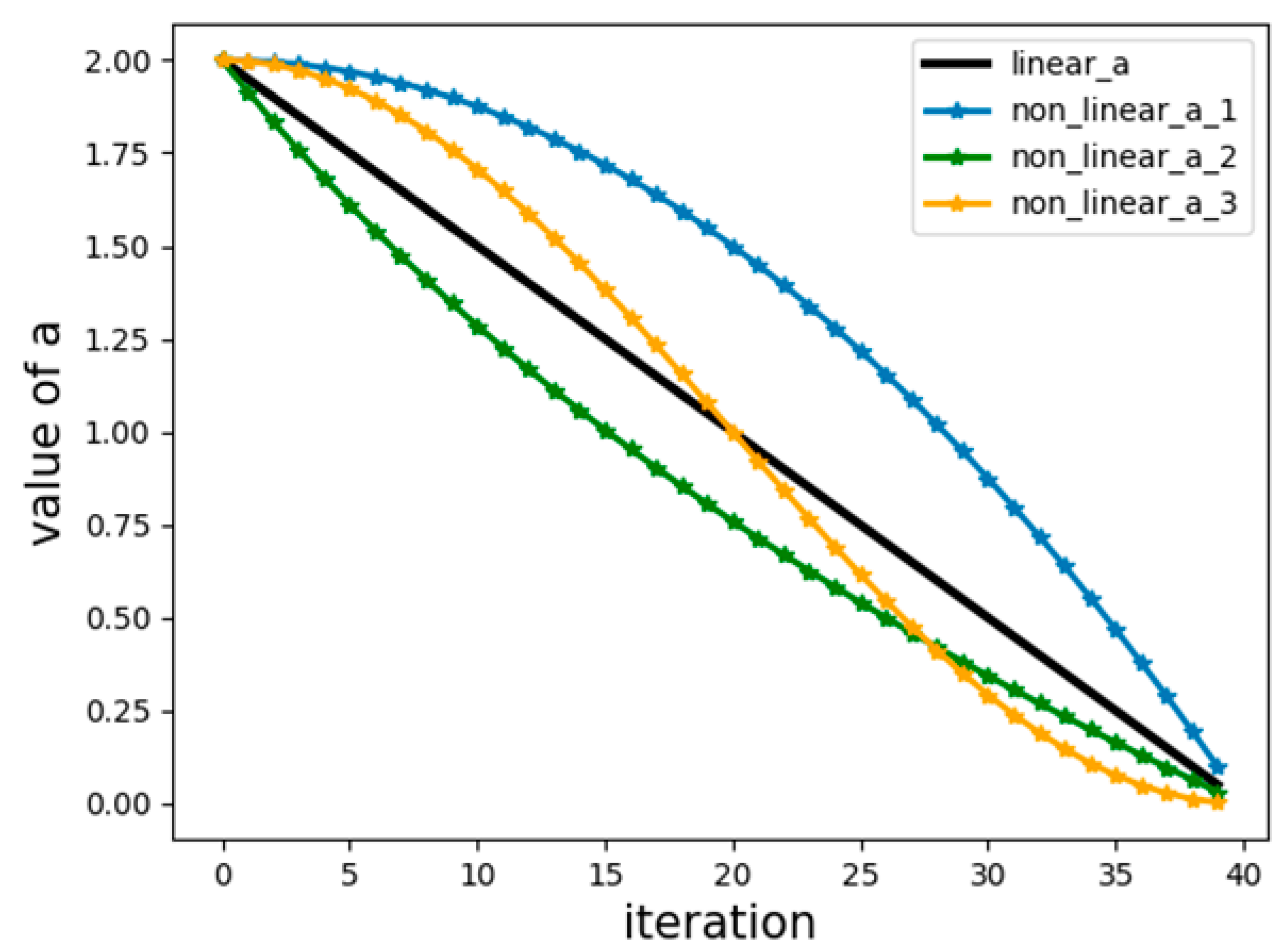
A comparison of the decay curves of $\overrightarrow{a}$ linear decreasing strategy, several other nonlinear decreasing strategies, and the nonlinear decreasing strategy proposed in this paper is given in Figure 5.

It can be seen from Figure 5 that, compared with the original linear decline strategy, the first half of “non_linear_a_1” has a slow decay rate, and the second half has a fast decay rate, which places more emphasis on local exploitation. In contrast, “non_linear_a_2” is just the opposite, placing more emphasis on global exploration. The improved strategy combines their advantages of them, reducing the decay speed of the first half and accelerating the decay speed of the second half, respectively, as shown in “non_linear_a_3”. The improved decay strategy balances global exploration and local exploitation and increases global exploration ability and convergence speed in the later period.

In the location update equation of the traditional GWO algorithm, information about the current position of alpha (α) wolf (global optimal solution), beta (β) wolf, and delta (δ) wolf agents are shared with the next generation of agents. As a result, the lack of diversity among agents causes the iterative process to fall into a local optimum easily. The individual historical best information is not systematically utilized in the algorithm. Therefore, GWO is a population-based memoryless stochastic optimization technique. In this paper, we propose a new memory-guided location update criterion based on the global best (${\overrightarrow{X}}_{gbest})$ location and individual historical best location (${\overrightarrow{X}}_{pbest}$).

The memory-guided location update equation proposed in this paper is calculated as follows:

$$\overrightarrow{X}\left(t+1\right)=w·\frac{\overrightarrow{X_1}+\overrightarrow{X_2}+\overrightarrow{X_3}}{3}+c_1·r_1·\left({\overrightarrow{X}}_{pbest}-\overrightarrow{X}\right)+c_2·r_2·\left({\overrightarrow{X}}_{gbest}-\overrightarrow{X}\right)$$

(21)

where t is the current iteration number. $r_1$ and $r_2$ are both random numbers uniformly distributed between [0,1]. $c_1$ and $c_2$ denote the individual learning factor and global learning factor, both between [0,1], which take the value of 0.5 in this paper. ${\overrightarrow{X}}_{pbest}$ and ${\overrightarrow{X}}_{gbest}$ denote the local optimal solution and the global optimal solution in the iterative process. w denotes the inertia weight, similar to the particle swarm algorithm, the size of w decreases linearly from the initial value ($w_{initial}$) to the final value ($w_{final}$), and the values taken in this paper are 0.9 and 0.1, respectively, and the calculation formula is as follows.

$$w=\frac{Maxiter-t}{Maxiter}\times \left(w_{initial}-w_{final}\right)+w_{final}$$

(22)

3.3.2. IGWO Optimizes the Objective Function

The improved IGWO is mainly used to optimize the objective function proposed previously. Given the gray wolf population and the maximum number of iterations to the NMPC controller, they are recorded as SearchAgentsNum and Maxiteration, respectively. The initial state of the objective function is marked as the initial position of the wolf population. The top three wolves with the best fitness are searched iteratively by inputting all gray wolf populations into the objective function for calculation. Since the objective function constructed above mainly represents the performance of position error on UUV trajectory tracking, when the objective function value reaches the minimum, the alpha (α) wolf in the corresponding population can be regarded as the current optimal solution. This way, the controller compares the maximum number of iterations, synthesize the results of multiple iterations, and selects an optimal result from the historical optimal solution and the current optimal solution as the output.

Algorithm of the whole optimization solution process is as follows (Algorithm 1).

Algorithm 1. Pseudo code IGWO to optimize the objective function

Input SearchAgentsNum, MaxIteration, ObjectiveFunction

Initialize grey wolf population, and $\overrightarrow{a}$, $\overrightarrow{A}$ and $\overrightarrow{C}$

Update the position of the initial gray wolf population

While (num < SearchAgentsNum) Calculate the fitness of gray wolf individuals according to the ObjectiveFunction,   and preserve the top three wolves with the best fitness as alpha (α), beta (β) and   delta (δ)

While (iteration < MaxIteration)   Update the current position of Grey Wolf   Update $\overrightarrow{a}$, $\overrightarrow{A}$ and $\overrightarrow{C}$   Calculate the fitness of all gray wolves   Update fitness and position of alpha (α), beta (β) and delta (δ)

Output position of alpha (α)

3.4. Stability Analysis of NMPC

As a control algorithm for rolling optimization solutions in the finite time domain, NMPC has been successfully applied in the industry since the late 1980s. The stability of model predictive control has been gradually proved, and ideas on different bases have emerged. This paper mainly adopts adding terminal constraints [29,30].

Here we consider a general model of controlled object:

$$x\left(k+1\right)=f\left(x\left(k\right),u\left(k\right)\right)$$

(23)

where $x\left(k\right)$ represents the state quantity of the robot at time k; $u\left(k\right)$ represents the control amount at time k.

The control function of each cycle is to solve the following optimization proposition:

$$V(k)={\displaystyle \sum _{i=1}^{N}l(\widehat{x}(k+i|k),\widehat{u}(k+i-1|k))}$$

(24)

where N represents the prediction time domain, and $\ell \left(x,u\right) \ge 0$, when and only when $x=0$, $u=0$, $\ell \left(x,u\right)=0$ is true. We can set up a nonlinear predictive control terminal constraint set optimization method, and introduce new variables into the optimization problem to reduce the conservatism of solving terminal constraint conditions. In addition, it can theoretically ensure that a wider range of terminal constraint sets ${\chi }_f$ can be obtained [31]. The terminal constraint set is guaranteed to be a positive invariant set under the effect of terminal control law. For general MPC, it is equivalent to the zero point as the end point; thus, we may add a terminal constraint here:

$$\widehat{x}(k+N|k)=0$$

(25)

For simplicity, it may be assumed that the control time domain and prediction time domain are equal and set to N, and it should be noted that $x$ and $u$ here are both constrained, that is:

$$\widehat{u}(k+i|k)\in U,\widehat{x}(k+i|k)\in X$$

(26)

where $U$ and $X$ are non-empty sets containing distant points. At the same time, we assume that $u=0$ and $x=0$ are an equilibrium state of the system, that is $0=f\left(0,0\right)$. And at each moment, the corresponding optimal sequence is obtained by solving: $\left\{u^0\left(k+i|k\right):i=0,1,2,\dots ,N-1\right\}$, only the first control action $u^0\left(k|k\right)$ is applied to the object. Then suppose that the optimization proposition of each cycle has a feasible solution and can be solved to obtain the global optimum, then we can assume that the system is stable at $u=0$ and $x=0$.

The proof of stability here adopts the traditional Lyapunov stability proof in the control theory, that is, to find a Lyapunov function of the system, which is positive definite, and its reciprocal is negative definite (the function value decreases). The idea here is to take the optimal value ($V^0\left(k\right)$) of the objective function of the optimization proposition in each period as the Lyapunov function. The positive definiteness of $V^0\left(k\right)$ has been explained in the previous assumptions. What we need to prove now is the negative definiteness of its reciprocal, that is, $V^0\left(k+1\right)\le V^0\left(k\right)$. As the same as other stability-proof methods, it is assumed that the model is unbiased and does not consider noise interference. Therefore, the predicted system state is consistent with the actual object state, if $u\left(k+i\right)=\hat{u}\left(\left.k+i\right|k\right)$ then $x\left(k+i\right)=\hat{x}\left(\left.k+i\right|k\right)$. Thus, they are:

$$\begin{array}{ll}{V}^0\left(k+1\right)& =\underset{u}{\min }{\displaystyle \sum _{i=1}^N\ell \left(x\left(k+i+1\right),u\left(k+i\right)\right)}\\ & =\underset{u}{\min }\left\{{\displaystyle \sum _{i=1}^N\ell \left(x\left(k+i\right),u\left(k+i-1\right)\right)-}\ell \left(x\left(k+1\right),u\left(k\right)\right)+\ell \left(x\left(k+1+N\right),u\left(k+N\right)\right)\right\}\\ & =-\ell \left(x\left(k+1\right),u\left(k\right)\right)+\underset{u}{\min }\left\{{\displaystyle \sum _{i=1}^N\ell \left(x\left(k+i\right),u\left(k+i-1\right)\right)}+\ell \left(x\left(k+1+N\right),u\left(k+N\right)\right)\right\}\\ & \le -\ell \left(x\left(k+1\right),u^0\left(k\right)\right)+V^0\left(k\right)+\underset{u}{\min }\left\{\ell \left(x\left(k+1+N\right),u\left(k+N\right)\right)\right\}\end{array}$$

(27)

We can ensure that $\underset{u}{\min }\left\{\ell \left(x\left(k+1+N\right),u\left(k+N\right)\right)\right\}=0$ based on the above formula, according to the terminal constraint in Equation (20) above. At the same time, according to $\ell \left(x\left(k+1\right),u\left(k\right)\right)\ge 0$, we prove that $V^0\left(k+1\right)\le V^0\left(k\right)$. Therefore, $V^0\left(k\right)$ is a Lyapunov function of the original system, and the Lyapunov stability of the original system at the origin can be verified. From this, we can preliminarily analyze that the stability of NMPC is reliable.

4. Simulation Analysis

The system model of the UUV is constructed according to the kinematics and dynamics model of the underwater vehicle. The NMPC controller is built according to the system model of the vehicle in the ROS environment and is verified in the UUV simulator environment.

4.1. Simulation Environment of Trajectory Tracking Control Based on ROS

The UUV simulator is an extension of underwater scenes developed on the open-source robot simulator Gazebo [32]. The plug-in developed is used to simulate underwater statics and hydrodynamic effects, thrusters, sensors and external interference, etc. Combined with the controller, the multi-machine cooperation of the UUV and the simulation of various underwater tasks can be realized [33]. The object of the study is the simulation vehicle “rexrov” provided by the uuv simulator.

The architecture of the NMPC constructed under the UUV simulator is shown in Figure 6, and its specific implementation process is as follows:

(1)

The NMPC predicts the state in the prediction time domain according to the reference point information and subscribes to the sensor data published by the “/gazebo” node.

(2)

In order to ensure the accuracy of the NMPC, the error between the prediction state and the feedback state is adaptively adjusted through the established objective function.

(3)

In the NMPC optimization stage, the improved IGWO algorithm is used to optimize the objective function to obtain the corresponding control law, which is released to “/rexrov/thruster_allocator” node as the actual output.

(4)

The node obtains the control signal of each thruster through the power distribution equation of UUV to control the UUV to move to the next position. Scroll the loop until the whole trajectory tracking process is completed.

In Figure 6, the marine environment node, data acquisition node, thrust distribution node, and controller node are started simultaneously in the ROS environment. Through the publication and subscription of the corresponding topic messages between nodes, the closed-loop control of the NMPC controller on the trajectory tracking task is completed. Given a reference trajectory message, the trajectory tracking control simulation of the UUV underwater can be implemented.

4.2. Tracjectory Tracking Comparison Results and Analysis

To verify the general applicability of the NMPC for trajectory tracking control, two reference trajectories are used to test the tracking effectiveness of the controller.

The first trajectory (case I) is a quadratic trajectory in the horizontal plane:

$$s_1\left(t\right)=\left\{\begin{array}{c}x=0.5t\\ y=0.1·{\left(0.5t\right)}^2\end{array}\right.$$

The second trajectory (case II) is a sine function trajectory:

$$s_2\left(t\right)=\left\{\begin{array}{c}x=0.5t\\ y=2·sin\left(0.5t\right)\end{array}\right.$$

The simulated trajectory tracking control effects for the two cases are shown in Figure 7 and Figure 8.

In Figure 7 and Figure 8, the whole moving process is relatively stable and meets the tracking control of the corresponding trajectory. The designed NMPC can generally meet the tracking control effect for different expected trajectories in the presence of hydrodynamic effects and current disturbances. The tracking errors are shown in Figure 9.

According to Figure 9, for different reference trajectories, when the average optimization time in case I reaches about 2 s, the tracking error of track tracking control in the x-direction is basically stable at about 0.25 m. When the average optimization time in case II reaches about 1 s, the tracking error of track tracking control in the x-direction is basically stable at about 0.3 m. Secondly, although there are different error fluctuations with the change of the track in the x and y directions, according to the test data statistics, the mean square deviation of tracking error in the x and y directions in case I is 0.043 m and 0.129 m, respectively, and the mean square deviation of tracking error in the x and y directions in case II is 0.017 m and 0.213 m, respectively. Within a certain allowable range of error, it basically meets the stability requirements of control performance.

To further analyze the control performance of the designed NMPC controller under different trajectory tracking controls, the tracking effect of UUV on the XOY plane under 10 groups of reference trajectories (including the above two groups of cases) is tested. Figure 10 shows the tracking effects of the other groups of cases. At the same time, the tracking error of UUV in horizontal x and y coordinates is analyzed. On the one hand, the trajectory tracking error reflects the accuracy of UUV in trajectory tracking control. On the other hand, for real-time optimal control, such as trajectory tracking control, the current state will affect the next state; thus, the control tracking error range is significant. Each group of tests was independently conducted 50 times. The absolute value and covariance of the maximum tracking error in the x and y directions of the 50 trials were averaged to obtain the following test record tables. The average of the absolute value of the maximum tracking error in each direction is shown in

Table 1. Table of maximum absolute tracking error in each direction.

Reference Tracking	Max Error-X 1	Max Error-Y 2
$s_1\left(t\right)=\left\{\begin{array}{c}x=0.5t\\ y=0.1·{\left(0.5t\right)}^2\end{array}\right.$	0.383	0.348
$s_2\left(t\right)=\left\{\begin{array}{c}x=0.5t\\ y=2·sin\left(0.5t\right)\end{array}\right.$	0.403	0.384
$s_3\left(t\right)=\left\{\begin{array}{c}x=0.5t\\ y=\sqrt{{7.5}^2-\left({\left(0.5t-7.5\right)}^2\right)}\end{array}\right.$	0.398	0.221
$s_4\left(t\right)=\left\{\begin{array}{c}x=0.5t\\ y=0.5t+sin\left(0.5t\right)\end{array}\right.$	0.381	0.378
$s_5\left(t\right)=\left\{\begin{array}{c}x=0.5t\\ y=0.5t+cos\left(0.5t\right)\end{array}\right.$	0.376	0.269
$s_6\left(t\right)=\left\{\begin{array}{c}x=0.5t\\ y=0.5t-sin\left(0.5t\right)\end{array}\right.$	0.328	0.367
$s_7\left(t\right)=\left\{\begin{array}{c}x=0.5t\\ y=0.5t-cos\left(0.5t\right)\end{array}\right.$	0.338	0.379
$s_8\left(t\right)=\left\{\begin{array}{c}x=0.5t\\ y=0.5t·sin\left(0.5t\right)\end{array}\right.$	0.326	0.362
$s_9\left(t\right)=\left\{\begin{array}{c}x=0.5t\\ y=0.5t·cos\left(0.5t\right)\end{array}\right.$	0.348	0.383
$s_{10}\left(t\right)=\left\{\begin{array}{c}x=0.5t\\ y=\ln \left(0.5t\right)-0.5t+1\end{array}\right.$	0.228	0.394

¹ Maximum absolute error of tracking error in x direction; ² maximum absolute error of tracking error in y direction.

. The average value of covariance in each direction is shown in

Table 2. Table of tracking error covariance in each direction.

Reference Tracking	Cov Error-X 1	Cov Error-Y 2
$s_1\left(t\right)=\left\{\begin{array}{c}x=0.5t\\ y=0.1·{\left(0.5t\right)}^2\end{array}\right.$	0.043	0.129
$s_2\left(t\right)=\left\{\begin{array}{c}x=0.5t\\ y=2·sin\left(0.5t\right)\end{array}\right.$	0.017	0.213
$s_3\left(t\right)=\left\{\begin{array}{c}x=0.5t\\ y=\sqrt{{7.5}^2-\left({\left(0.5t-7.5\right)}^2\right)}\end{array}\right.$	0.042	0.193
$s_4\left(t\right)=\left\{\begin{array}{c}x=0.5t\\ y=0.5t+sin\left(0.5t\right)\end{array}\right.$	0.004	0.144
$s_5\left(t\right)=\left\{\begin{array}{c}x=0.5t\\ y=0.5t+cos\left(0.5t\right)\end{array}\right.$	0.011	0.235
$s_6\left(t\right)=\left\{\begin{array}{c}x=0.5t\\ y=0.5t-sin\left(0.5t\right)\end{array}\right.$	0.037	0.135
$s_7\left(t\right)=\left\{\begin{array}{c}x=0.5t\\ y=0.5t-cos\left(0.5t\right)\end{array}\right.$	0.051	0.198
$s_8\left(t\right)=\left\{\begin{array}{c}x=0.5t\\ y=0.5t·sin\left(0.5t\right)\end{array}\right.$	0.009	0.228
$s_9\left(t\right)=\left\{\begin{array}{c}x=0.5t\\ y=0.5t·cos\left(0.5t\right)\end{array}\right.$	0.134	0.139
$s_{10}\left(t\right)=\left\{\begin{array}{c}x=0.5t\\ y=\ln \left(0.5t\right)-0.5t+1\end{array}\right.$	0.002	0.147

¹ Average covariance of tracking error in x direction; ² average covariance of tracking error in y direction.

.

4.3. Comparison and Analysis of NMPC Optimization Algorithms

In addition to verifying the universal applicability of the designed NMPC controller on different reference trajectories, this paper also compares the NMPC tracking effect of the improved IGWO with the SQP optimization algorithm, traditional GWO algorithm, and the sparrow algorithm (SSA). Figure 11 and Figure 12, respectively, show the tracking effect diagram and the tracking error diagram in the x and y directions of the controller of each algorithm when the expected trajectory is sinusoidal (case II).

According to Figure 11, the IGWO can control the decay rate of the convergence factor from fast to slow, which increases the global exploration ability in the early stage and improves the convergence rate in the later stage. By observing the first peak of the function in the figure, it can be seen that the transition of the tracking path of the IGWO controller at the peak of the function is smoother, reducing the path fluctuation caused by local optimization, and making the UUV more adaptive when the course changes sharply. From the perspective of global trajectory tracking effect, the tracking effect of the IGWO controller is less volatile and the control effect is more stable than other algorithm controllers.

To better analyze the performance of the improved algorithm in tracking error, the maximum tracking error and tracking error covariance of the above algorithms in all directions are recorded in

Table 3. Table of tracking error covariance in each direction of algorithms.

Optimization Algorithm	Cov Error-X 1	Cov Error-Y 2
IGWO	0.0173	0.213
GWO	0.0284	0.224
SSA	0.0534	0.249
SQP	0.0398	0.255

¹ Average covariance of tracking error in x direction; ² average covariance of tracking error in y direction.

and

Table 4. Table of maximum absolute tracking error in each direction of algorithms.

Optimization Algorithm	Max Error-X 1	Max Error-Y 2
IGWO	0.343	0.384
GWO	0.472	0.783
SSA	0.515	0.467
SQP	0.524	0.778

¹ Maximum absolute error of tracking error in x direction; ² maximum absolute error of tracking error in y direction.

respectively:

By analyzing the data in Figure 12 and the above tables, it can be seen that the tracking control of the IGWO algorithm in the x-direction can reach a stable error range faster, which only takes about 1 s on average, whereas the SQP algorithm takes about 2 s, and the GWO algorithm takes about 2.5 s. Secondly, the error range of the IGWO is more stable in both the x direction and the y direction. The average covariance of tracking error in x-direction is 0.0173 m, whereas the average covariance of tracking error in the direction of SQP, GWO and SSA are 0.0398 m, 0.0184 m and 0.0534 m, respectively. Compared with other algorithms in tracking error fluctuations in the x and y directions, the maximum absolute tracking error of the IGWO in the x direction is much smaller, only 0.343 m, whereas the maximum absolute tracking error of GWO, SQP and SSA in this direction is 0.472 m, 0.515 m and 0.524 m, respectively. The maximum absolute tracking error of the IGWO in the y direction is also much smaller, only 0.384 m, whereas the absolute value of the maximum tracking error of SQP and GWO in this direction is 0.778 m and 0.783 m. It can be seen that the improved algorithm is relatively more stable and accurate in the global track tracking effect.

In addition, the sampling time of the UUV controller and the data release frequency of the Gazebo in the UUV environment should be consistent as much as possible, which has strict requirements for the optimization speed of the controller. According to the experimental records, the IGWO-NMPC only needs to set the population number and maximum iteration number to 20 and 30 to satisfy the requirement. However, the GWO-NMPC satisfies the trajectory tracking requirement under the condition that the population number and maximum iteration number are 30 and 40, respectively. The population and maximum iteration numbers of SSA-NMPC under the exact requirement are 50 and 80, respectively. Moreover, the SQP optimization algorithm is difficult to adjust the algorithm’s parameters in different experimental environments; therefore, it is difficult to ensure the stability of the trajectory control effect. In this regard, the IGWO controller has a more robust global search ability and can reach the stable error range faster. Moreover, the optimization speed is faster and performs better in real-time control. It can perform online parameter adjustment under complex working conditions; thus, the tracking performance is better in harsh working conditions.

5. Conclusions

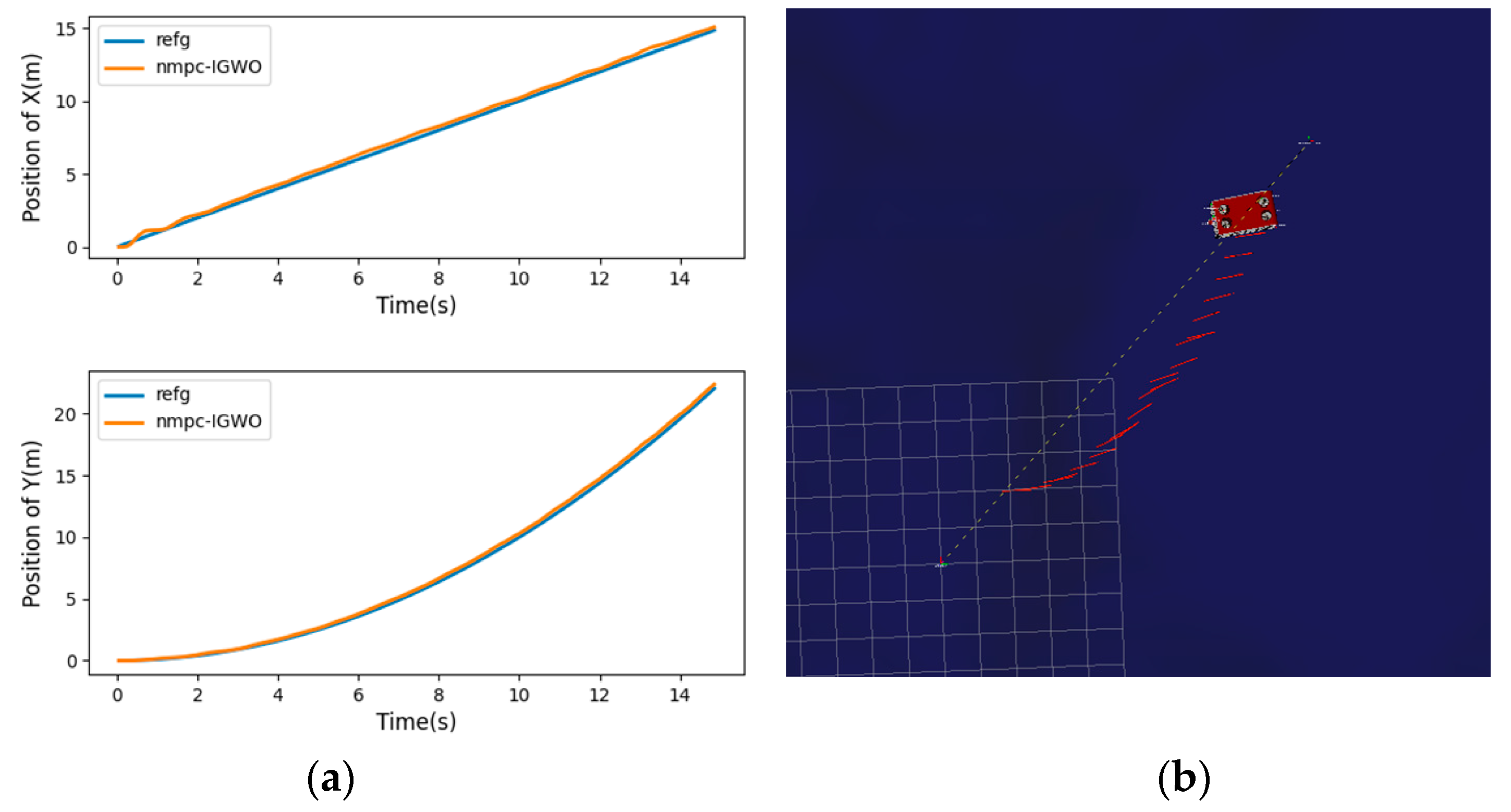
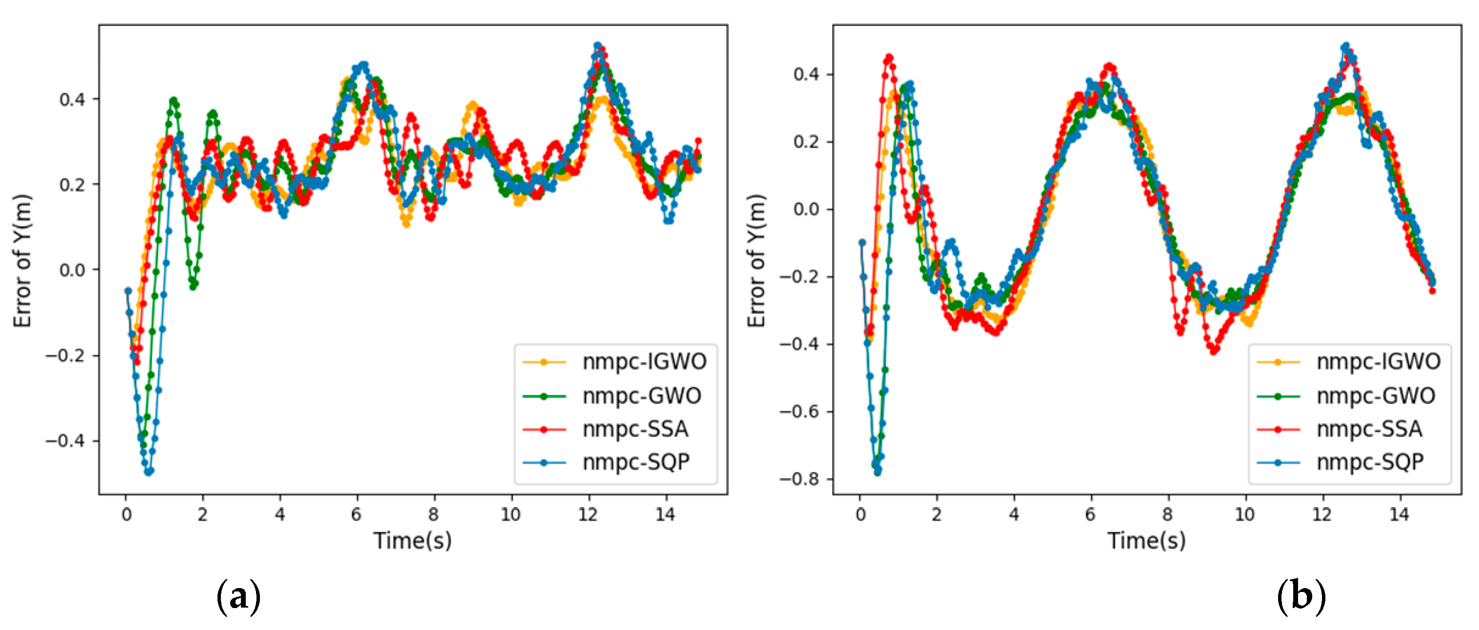
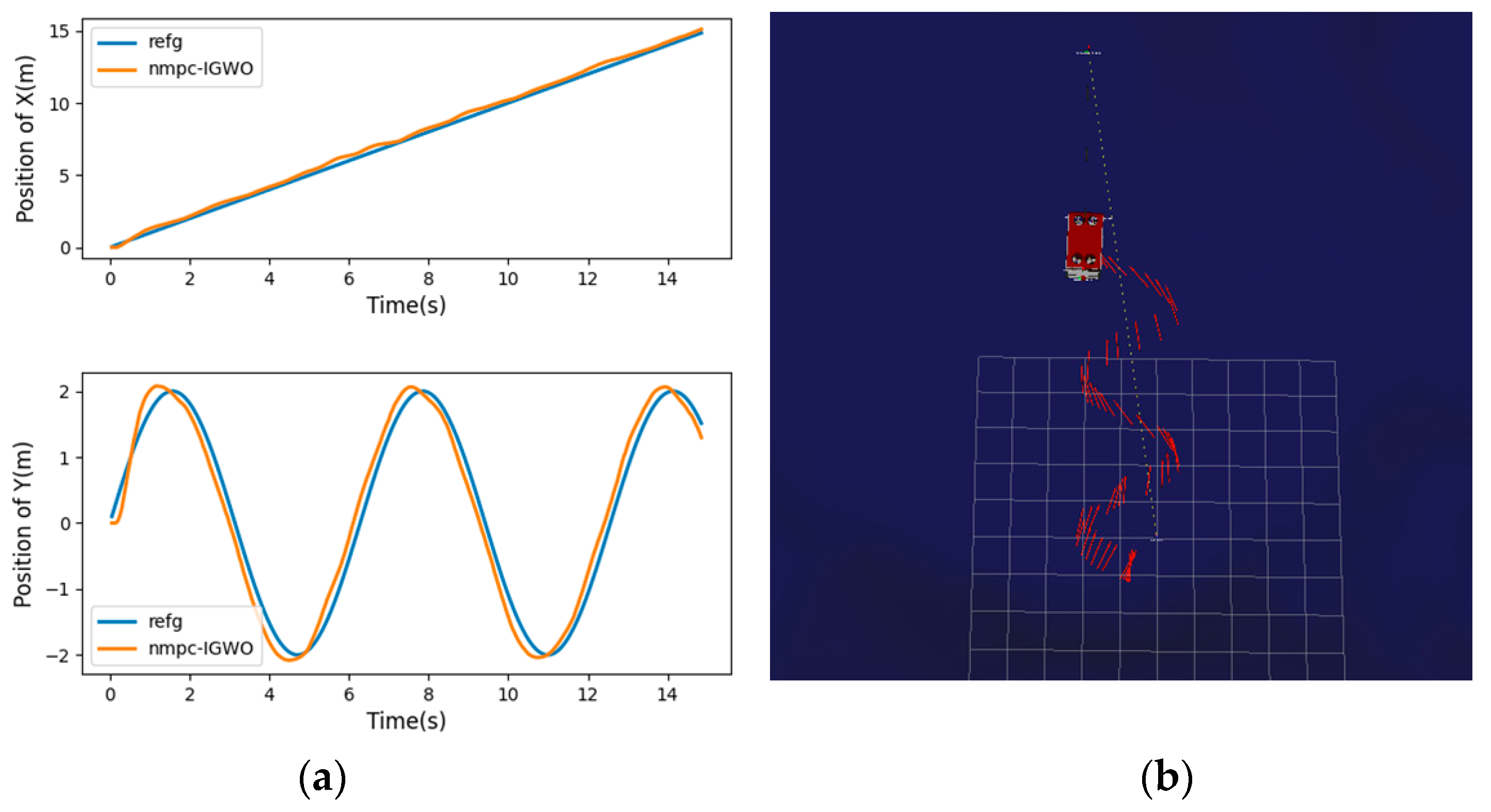
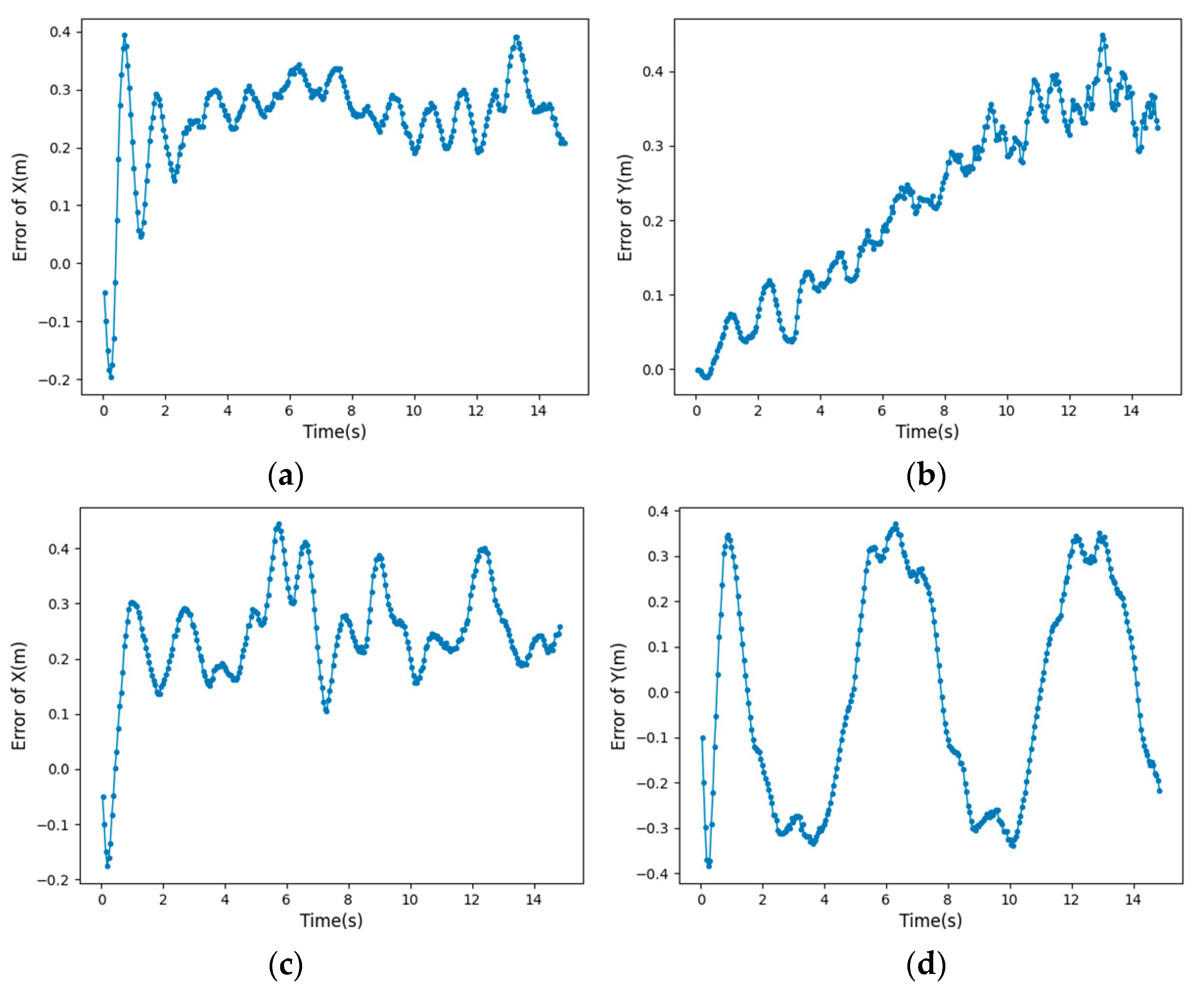
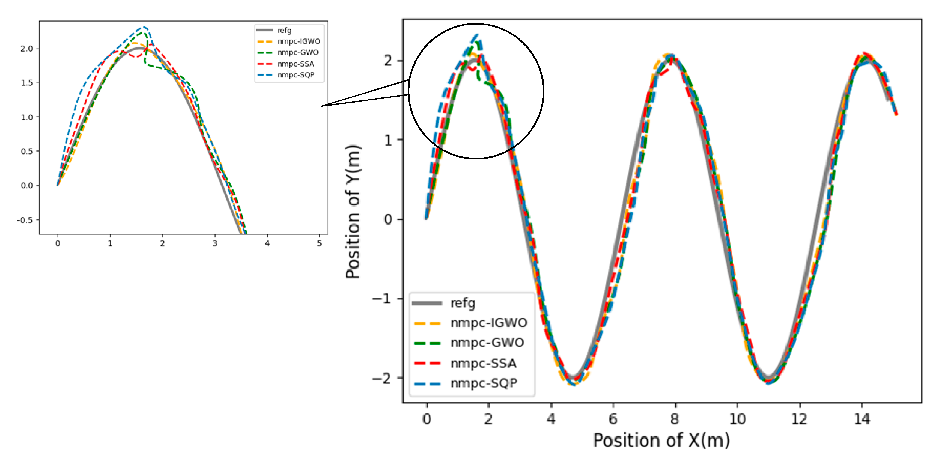
This paper proposes a new IGWO-NMPC trajectory tracking algorithm for UUVs, which combines NMPC with an improved GWO algorithm with nonlinear decay. The NMPC is used to adjust the prediction error of the UUV’s future state, and the decay rate of the convergence factor is controlled from fast to slow, which increases the global exploration ability in the early stage and improves the convergence rate in the later stage. It effectively reduces the fluctuation range of tracking error and the time required for stability. The problems such as the insufficient stability of the trajectory tracking controller of the UUV and the poor real-time performance of the NMPC are solved. The simulation experiments of tracking different trajectories show that the IGWO-NMPC has universal applicability and high tracking performance in trajectory tracking control.

In marine environment exploration and other tasks, the UUV is affected by the unknown underwater environment on the one hand, and on the other hand, UUV is a nonlinear system with multiple degrees of freedom and strong coupling, which makes the task execution difficult. As one of the key technologies of UUV, trajectory tracking control is widely used in the fields of autonomous operation and automatic control, and can effectively solve the exploration tasks in the unknown ocean field and other harsh environments that are not convenient for personnel to carry out. The research of this paper is devoted to designing a nonlinear model predictive controller, and proposes an improved optimization algorithm for the controller. It can more restore the control effect of UUV, and solve the problems such as the insufficient stability of the trajectory tracking controller of the UUV and the poor real-time performance of the NMPC. In addition, how to make new improvement attempts on the traditional framework and objective function of NMPC, and apply the improved trajectory tracking controller to the reliable vehicles. At the same time, explore how to combine with other decision-making technologies such as trajectory planning to realize the autonomous navigation control of UUV. And the experimental verification in underwater missions will be the goal of our future work.