Abstract
The fault detection method (FDM) plays a crucial role in controlling and operating microgrids (MGs), because it allows for systems to rapidly isolate and restore faults. Due to the fact that MGs use inverter-interfaced distributed production, conventional FDMs are no longer appropriate because they are dependent on substantial fault currents. This study presents a smart FDM for MGs based on the Hilbert–Huang transform (HHT) and deep neural networks (DNNs). The suggested layout aims to prepare the fast detection of fault kind, phase, and place data to protect MGs and restore services. The HHT pre-processes the branch current measurements obtained from the protective relays to extract the characteristics, and singular value decomposition (SVD) is used to extract some features from intrinsic mode functions (IMFs) that are obtained from HHT to use as input of DNNs. As part of the fault data development, all the information eventually enters the DNNs. Compared with prior studies, this suggested method provides considerably superior fault-type identification accuracy. It is also possible to determine new fault locations. A detailed assessment analysis of this suggested FDM was conducted on IEEE 34-bus and MG systems to demonstrate its effectiveness. The simulations indicated that the proposed method is effective for detecting precision, computing time, and robustness to measurement uncertainties.
1. Introduction
As energy demand increases, environmental concerns arise, and as fossil fuel reserves run out, renewable energy sources emerge as a solution. Consequently, microgrids (MGs) have been developed to integrate distributed energy sources into electrical networks [1]. Numerous studies have addressed or compensated for the intermittent nature of renewable energy resources. Other problems associated with MGs include the grid and MG faults. When the design of electrical systems is inadequate, faults seriously harm the electrical components and result in costly malfunctions. In most cases, protection against faults is controlled at the point of common coupling (PCC) through the static switch, allowing for the MG to be isolated from the main grid in the event of a fault. In fault detection methods (FDMs), the goal is to obtain data on the fault signal in various cases [2]. The aim is to implement methods for fault detection (FD) and diagnosis in real time by applying a relatively inexpensive controller that is highly reliable for static switches [3].
In terms of operational concerns, protecting MGs is a significant issue [4,5]. As renewable energy resources become more prevalent in current energy grids, MGs tend to be connected to inverter-interfaced distributed generations (IIDGs), including battery energy storage systems (BESSs) and photovoltaic (PV)-distributed generation (DG). Fault currents can overwhelm conventional protection relays for FDMs in distribution systems. Nevertheless, IIDGs produce small fault currents that prevent the activation of protective mechanisms [6]. Therefore, the MGs are not protected by such relays. In [7], the current and voltage dynamics of the MGs were thoroughly examined.
In general, there are three purposes of FDMs in an MG. In the event that a fault occurs, the FDM identifies the fault type (FT), fault phase in asymmetric FTs, and fault location (FL). In the first two cases, additional fault isolation procedures are possible, whereas in the subsequent case, service restoration is possible. Ref. [7] advocated integrating single-phase protection equipment to maintain sound phases during imbalanced short-circuit faults. A selective phase trip can be achieved using precise FT and phase data. Thus, the reliability of the systems is dramatically enhanced, and utility companies have increasingly adopted a protective approach. In addition, the exact diagnosis of FLs significantly decreases the work required for utility service restoration [8], which is particularly important when underground work is involved.
Information-based and digital signal processing methods have recently become increasingly popular for MG FTs and phase detection. For example, decision trees and random forests have been used extensively to diagnose faults in on-grid and off-grid MGs [6]. In addition, FDM was studied using support vector machines and the k-nearest neighbor method [4]. These data-based methods provide near real-time fault classification (FC), owing to their high computational capabilities. Moreover, digital signal processing methods, such as the discrete Fourier transform, wavelet transform (WT), and Hilbert–Huang transform (HHT), have been extensively used for preprocessing the input signal to extract the time-frequency features for evaluation [4,6,9]. Readers seeking more information on MG FDM surveys can find it in [6].
According to refs [10,11], HHT can be used to reduce the dimensionality of a signal and decompose it. In general, HHT involves two stages: Firstly, applying an information-driven decomposition method called empirical mode decomposition (EMD), and secondly, implementing Hilbert spectral analysis (HSA) on the decomposed signals, called intrinsic mode functions (IMFs). In addition to all of these features, EMD is able to offer numerous enhancements over Fourier analysis, including the ability to automatically and adaptively extract oscillations from each signal; furthermore, this is straightforward to execute; and in addition, it is robust enough to cope with all non-linear and non-stationary signals. Additionally, EMD effectively captures non-linear features of amplitude and frequency modulation at local time scales. During IMFs, Hilbert spectral assessments give frequency information that is crucial to assessing non-stationary signals.
The characteristics of static switch methods were examined, along with various algorithms and methods for FDMs. Ref [1] utilized an FPGA board for the FDMs and FLs of a static switch. Controlled by the six-layer adaptive network-based fuzzy inference system (ANFIS), the static switch next to the PCC is activated [1]. The WT was utilized in ref. [2] to adopt the features of the current waveform at the relaying spots, and a decision tree was then employed to conduct the FDM and FC. The HHT uses three machine learning schemes, such as support vector machine, naive Bayes classifier, and extreme learning machine, which were applied in ref. [3] to diagnose and discern faults by applying three-phase current waveforms at the goal buses of various MG feeders. Three switch technologies, IGBT-driven, SCR-driven, and circuit-breaker-driven switches, were examined in ref. [12]. A DSP was incorporated with a prototype switch to control the relays, datum acquisition, and communication. The Takagi–Sugeno–Kang fuzzy rule-driven method was examined in [13] to design a static switch. In [14], three deep neural networks (DNNs) were incorporated with WT to develop an FDM, FL, and FC layout of the MG, including numerous branch currents. However, the static switch has not been discussed. According to ref. [15], only the scheme components of three-phase voltage values are used to locate faults in smart grids. A graph analytic-driven algorithm identifies the faulty lines by contributing system topology and attributing affinity values to the quest space to identify the affected areas by the fault. Using a wavelet multiresolution evaluation of the associated scheme components, heuristic indices have been used to identify the faulty lines within the faulty areas.
Moreover, FDM, FC, and FL play critical roles in protecting the bulk/DC grid [16,17,18,19,20]. In [16], an FDM approach to transmission lines (TLs) was proposed according to the sum of the squared three-phase current and the moving mean method. A Petri net was examined in [17] to detect faults in energy transmission systems. The spatiotemporal data network according to phasor measurements for FDM in a transmission system was examined in [18]. A WT was used to diagnose faults in a DC MG [19]. A neural network (NN) and wavelet transform were examined in [21] to diagnose faults. A combination of ANFIS and Hilbert space according to the power setting was used to protect the MG [22]. In ref. [23], a new concrete characteristic-choosing approach is proposed to improve fault detection and cyber-attacks in power systems using mutual data.
However, MG–FDMs are lacking. Several studies do not include FT data; therefore, they cannot be effectively applied in the single-phase tripping paradigm. In addition, current research on FL detection (FLD) examines low-voltage DC MGs [24]. When AC distribution systems are used, FLD is usually accomplished using injection-driven or traveling-wave methods [8]. Many traveling-wave methods experience problems in detecting and discriminating reflected waves [24], and many require the synchronization of information through communication systems. They failed to demonstrate the effectiveness of FLD on islanded MG or loop/ring topologies. Injection-driven algorithms have been restricted to phase-to-ground faults and can merely be applied to radial grids [24].
The current study describes a smart FDM (SFDM), which uses HHT, singular value decomposition (SVD), and the latest advancements in DNNs, which are a category of information-based machine learning methods, to fill the knowledge gap for IIDG-equipped MGs. SVD is used to extract some features from IMFs and signal spectral energy that is obtained from the signal after it is processed by HHT to use as input of DNNs. Noise and power disturbances affect the HHT, but the DNN enhances the robustness through its ability to handle noisy information [25,26]. A diagram of the offered FDM is depicted in Figure 1. It uses the three-phase current magnitudes of a branch in a cycle gathered through a protection relay as the input information. Then, feature extraction was performed using HHT and SVD. Subsequently, the attributes and features (signal spectral energy and entropy of IMFs) were fed into three DNNs for fault-kind FC, fault-phase detection, and FLD. The fault data were then used to implement the subsequent protection and remedial control. This study makes the following contributions:
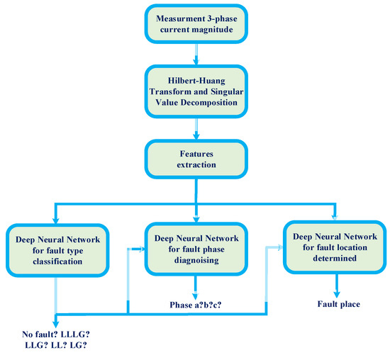
Figure 1.
A schematic of the MG–FDM.
- An FDM for AC MGs is proposed to provide precise and timely FT, phase, and place data;
- This study combined DNNs and HHT with SVD to solve the MG–FD problem from an information-based standpoint;
- Complete scenarios were performed to decompose the efficiency of the offered method and compare the outcomes with those of other methods.
This suggests that FDM is faster and more precise than the previous methods (type, phase, and place) because it does not rely on communication. Consequently, it adapts to various types of operations and topologies, including grid-connected, islanded, radial, and loop topologies. In addition, two traditional synchronous generators, as well as IIDGs, can handle energy dynamics.
Below is a summary of the remainder of the study. An analysis of the suggested layout is presented in Section 2. The HHT and SVD methods are presented in Section 3, and the FDM formulation is discussed in Section 4. Simulations are performed in Section 5 to demonstrate the effectiveness of the proposed method. Finally, Section 6 concludes the study.
2. Examined MG System
This study examines a revised MG system on the basis of the CERTS MG (CMG) [27] that is used in several prior studies on MG–FD, including ref. [4] and ref. [7]. Figure 2 shows that the installed MG runs at 480V, 60 Hz and supports loads in both non-islanded and islanded modes, depending on the status of the PCC switch. The elements in Figure 2 are described as follows: CB and R define the circuit breaker and relay, respectively. L and T define the load and transformer, respectively. Line defines the transmission line. The loop switch provides a means of operating the system in loop/radial networks. The offered method was tested on several types of DGs in MGs, including a BESS (DGBESS in Figure 2), a PV energy resource (DGPV), and a conventional diesel synchronous generator (DGSG). A current-controlled voltage resource inverter connects the DGBESS to the system, which is controlled by a frequency-controlled inverter in islanded operation. A current-controlled voltage resource converter connects the DGPV, maintaining its control method in islanded or grid-connected operations.
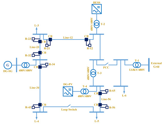
Figure 2.
An enhanced diagram of the CMG system.
Ref. [4] was used to determine the values of loads, transformers, and TLs, as depicted in Figure 2. There are four loads distributed with this network, namely 90 kW for all L_3 to L_6, as well as [45, 45, −40, −20] kVAr for L_3,L_4,L_5, and L_6 in nominal conditions, respectively. Lines [12, 23, 34, and 56] are of the [AWG2, AWG00, AWG2, and AWG2] with lengths of [68.58, 22.86, 68.58, 68.58] m, respectively.
Four power lines were investigated in this study, namely lines 12, 23, 34, and 56, as depicted in Figure 2. Due to the fact that the system consists of many DGs and that the MG operates in a loop topology, the two ends are protected by relays. By attaching a current transformer, the relays sampled the branch current magnitudes at a rate of 3.84 kHz, which is in agreement with the settings of this study.
3. Hilbert–Huang Transform
The HHT comprises HSA and EMD. The EMD is described as the basic part which divides the data set into smaller and restricted parts called IMFs. To obtain the instantaneous frequencies of the function, IMF Hilbert transforms were calculated [28,29].
3.1. Empirical Mode Decomposition
The sieving method extracts mono and symmetrical details from nonstationary and nonlinear signals. Sieving is the process of deleting the lowest frequency of information until only the highest is retained. IMFs were used to analyze the signals. When this satisfies the following two requirements, it displays an oscillating wave.
- For a data set, the number of zero crossings and extremes are assumed to vary or be equivalent to one;
- All points have a zero-average extent for the envelope defined by the local minimum and maximum.
To handle the IMF evaluation using EMD, the following steps were taken:
- 3.
- Explore the local maximum and minimum in the sample data, and build a pair of envelopes by connecting them using cubic splines;
- 4.
- Average was determined for the two envelopes. By subtracting it from the basic signal , the primary component is obtained as follows;
- 5.
- When satisfied the previous two requirements, it would be the initial IMF; otherwise, it would be the main function and stages ‘a’ to ‘c’ are repeated in order to obtain as follows:
- 6.
- When sifting is repeated times, the initial IMF is , ;
- 7.
- Leaving independent of and making it , as follows;
- 8.
- is regarded as the primary signal. Equation (1) to Equation (3) are repeated to calculate the next IMF.
The described process was repeated times, and similar IMFs were obtained. The stop criteria for the decomposition process would describe whether becomes a monotonic function that cannot be extracted by any further IMF.
3.2. Hilbert Transform
Due to the fact that IMFs are analytical subordinates, the Hilbert transform is used to create an instant frequency for all IMFs. The Hilbert transform for the time-domain signal is considered as the other time-domain signal, represented by , such that is considered as an analytical signal. The amplitude and phase are determined as follows:
The following formulas are used to determine the instant frequency and signal spectral energy in Equations (6) and (7), respectively:
3.3. Singular Value Decomposition
In this paper, SVD is used to extract some features from IMFs to use as input of DNNs. Singular value decomposition (SVD) would be a matrix decomposition way, breaking a matrix into three matrices. If and is the nonzero singular values of , based on [2], the SVD is as follows:
In which , and , Q shows a diagonal matrix, as follows:
Afterward, matrix diagonal elements ‘Q’ make , matrix ‘F’; thus, ‘Q’ would be
In which and shows the nonzero singular values for matrix .
3.4. Shannon Entropy
Using Shannon entropy in the time domain, the structure and pattern of examined information can be assessed. Therefore, wavelet entropy-driven signal evaluation is capable of indicating the frequency and time components of the signal.
Based on ref [30] and using , the likelihood would be
Lastly, the entropy has the following formulation:
4. DNN-Driven FD
DNNs are artificial NNs (ANNs) composed of several hidden layers of neurons placed between the inputs and outputs. A wide range of complex nonlinear systems have been modeled in engineering studies [25]. Furthermore, DNN computations only involve basic algebraic formulas, resulting in rapid calculations. Owing to this feature, a DNN can handle these issues in real time.
Due to the assumption that branch current measurements can provide an immediate indication of a system fault, a DNN-driven FDM has been suggested. This assumption has been widely accepted by researchers, as evidenced in [4,6,7], for example. Furthermore, the temporal dependency in the magnitudes of the sampled currents is also seen as a way to find faults. The following section constructs an SFDM using time-series branch current measurements, and the HHT characteristics elicited in Section 3.
Fault kind FC, fault phase detection, and FLD are the three parts of the FD subject. A DNN existed in each part. Figure 3 depicts the flow chart of the offered FDM. In the offered FDM, a protection relay in the MG is sampled in the three-phase branch current magnitudes at random intervals. HHT and SVD are used to process the results and extract their characteristics. These results and characteristics were later entered into an FC–DNN fault type. The FL was determined using the FLD–DNN when a fault was found. Moreover, when an unbalanced fault was detected, a fault-phase detection DNN was applied to extend the fault phase. Consequently, the gathered data are used in future decision-making procedures related to control operations, such as the recovery and isolation of faults.
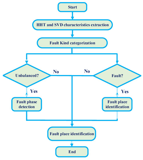
Figure 3.
The diagram of the offered SFDM.
The rest of this part introduces the method used to engender the three DNNs. Next, this section presents the architecture of the DNNs, the training information preparation process, and the training optimization formation.
4.1. Condensed Layer and GRU
This study mostly used a gated recurrent unit (GRU) to engender DNNs for handling the three parts of the MG–FD issue. GRU [31] is an updated version of an ANN, which is a widely employed data-mining and machine-learning method. Several fields have utilized ANNs owing to their non-model-dependent and computation-effective characteristics. An ANN simulates a control system model by examining the relationship between the inputs and outputs of a system.
By contrast, a conventional ANN ignores the time–domain relationship of the input information. GRU, as well as several DNNs, have been developed to combat such weaknesses. A GRU can maintain earlier data for future utilization and capture temporal dependencies in the input information through the introduction of extra recurring links in an NN’s hidden layers [31].
If is a time series, the GRU develops a sequence of output amounts based on the sequence of input amounts from to . This can be explained by the following architecture:
here, the element-wise product is denoted by , and the entire and matrices define the learning variables of the GRU. Equation (13) to Equation (16) show that GRU simulates the relation among output and input to by applying the learning variables whose amounts would not be known at first. In general, we use a pre-defined input, and the output information is used to tune such variables to show the relation. This procedure is known as training and is generally performed offline. Following training, it is possible to determine the expected output amount based on the number of learning variables, regardless of whether the real output can be predicted.
In addition to the GRU, the second crucial NN layer is a condensed or completely linked layer. The condensed layer (CL) contains many artificial neurons that calculate their output based on the input information as follows:
where is the input and is the output. The learning variables of the CL are and , and the activation function is represented by [26].
4.2. DNN Architecture
Three DNNs were used in the suggested SFDM for classifying FTs, identifying fault phases, and locating fault positions. GRU and standard completely interconnected neuron layers were used in each network. The models differed slightly due to their various outputs.
First, a fault-type FC–DNN was constructed. As inputs, the network uses three-phase current data and HHT-driven with SVD characteristics to determine whether a particular dynamic sequence represents the fault and FT. In accordance with earlier studies [4,6,7], the following FTs are considered: (i) single line-to-ground (LG), (ii) line-to-line (LL), (iii) two-line-to-ground (2LG), and (iv) three-lines to the ground (3LG). A total of four 0-1 indices represent the four FTs in the DNN output. Due to the fact that this DNN distinguishes between faults and sounds, an additional no-fault index is added to the output, increasing its length to five.
The DNN uses four GRU layers (GRULs) and three CLs to analyze the current data as well as HHT and SVD characteristics. In particular, the earliest GRUL maps the time series into the higher-dimensional domain, and the following two GRULs have been applied to extract the temporal dependencies of the input information. In the final layer of the GRU, the dependence is expressed as a one-dimensional vector, and the obtained HHT and SVD characteristics are integrated with it as input to the following condensed neuron layers. Finally, two CLs abstract the FT features, and the final layer transforms the abstracted characteristics into human-readable FTs. The greatest amount in the vector determines the FT. If the third element in the output vector is the greatest, this implies that a fault of the same kind is illustrated with the third output, such as 2LG, and occurred in the system. The next fault-phase detection DNN was applied to identify the fault phase for unbalanced faults (LG, LL, or 2LG). The DNN includes an output vector of length , where all the elements show the fault status of the phases. The fault phase is determined by the phase with the highest value in the output vector. The fault phases are those with the two greatest amounts in the cases of LL or 2LG faults. Finally, the FLD–DNN only produces one amount from the latest CL, representing the percentage location on the TL from the sampling protection relay. Figure 4 shows the final layers of the faulty line detection and FLD–DNNs.
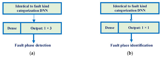
Figure 4.
The final condensed neuron layers of the faulty line detection and FLD–DNNs: (a) faulty phase detection; (b) FLD.
In the proposed DNN, three-phase current magnitudes are the sole inputs. It is possible that additional data, such as fault resistance, are accessible prior to identification in specific practical applications. As a result, these data serve as an updated input to the initial CL, so that the modeling is improved through the use of extra data.
4.3. Time-Series Simulation and Training
The DNNs created for the FD must be trained offline before the learning variables are used. Training information, including input-current magnitude measurements and output-fault data, is derived from historical information or by simulating various operating events over time. The input current magnitude measurements were as follows:
The current magnitude measurements of phases , , and are shown by , , and in the cycle, respectively. As the fault data are presented in the three DNNs, various outputs , and must be created for the three DNNs.
Based on a set of R training information , the learning variables in the DNNs were trained using several gradient descent algorithms [25]. Similar to FT, FC is a multinomial FC subject, and the multinomial cross-entropy loss function (LF) is used for optimization purposes. Similarly, the binary LF of the cross-entropy is allocated to the faulty line detection DNN owing to the poly-tagged FC feature. The LF of the FL–DNN is the LF of the average squared error [26].
It is possible to train hundreds of thousands of variables by using the proposed DNN framework. In the absence of overfitting, the simultaneous adjustment of their amounts is impossible [32]. As a result, a useful method, named “dropout,” has been used for addressing the problem [33]. Using this method, the output amounts of a neuron are adjusted to zero in a random manner using consumer-described likelihood. This prevents the network from excessively depending on certain neurons to generate outputs, because the dropped neurons do not participate in the computation. Thus, it is possible to extract additional robust characteristics during the learning process [32]. The “dropout” method would be exclusively used in the training procedure. The network output is generated if all neurons contribute to the developed variables [33].
This study employed an HHT, SVD, and DNN to construct an AC MG–FD model. With DNN, variable adjustment, a prolonged procedure, is performed offline, which makes it superior to the existing computing methods. Online tests involve minimal linear algebraic computations, which makes them computationally effective. Meanwhile, the HHT with SVD used in this study lacks a pre-processing stage to reduce the test time. Part 5-A illustrates that under normal conditions, the HHT is calculated sufficiently rapidly to keep the total system response time acceptable. With the rapid progression of signal-processing technologies, HHT algorithms can be rebuilt online to significantly decrease computation time. Online HHT with SVD algorithms are simply integrated into the suggested FD process, and there is no change in identification precision if the HHT outcomes remain unchanged.
5. Scenarios
Simulations are performed to evaluate the FD efficiency of the offered scheme. The FT/phase identification and FL precision were first evaluated, and then the outcomes were compared with those of existing methods. Subsequently, the effect of noisy measurements on the FD effectiveness was investigated. As a final step in evaluating the generalization of the offered scheme, it was examined on a different MG system outside the CERTS system.
Training the learning variables in a DNN using supervised learning requires adequate prior information regarding the post-fault/event energy dynamics. To tune the variables that approximate the behavior of the system, the training information must contain sufficient knowledge about various operational situations and events. In this study, training information was generated by applying a CMG system through time-series simulations of various network structures, grid-connected states, symmetric and asymmetric FTs, fault resistances, fault lines, loads, and FLs. Table 1 describes these settings in detail. Overall, 23,461 fault scenarios were generated and simulated in this paper. The variables are trained by constructing several sound scenarios. Table 2 describes these scenarios, and simulations were performed for 957 sound scenarios. For all created cases, the simulated branch currents served as sensor devices collected through the protection relays. Practically, utility companies can utilize previous operational information during training.

Table 1.
Configurations of fault scenarios.
Table 2.
Configurations of sound scenarios.
In the case of cross-validation and to avoid overfitting, the created fault and sound scenarios were randomly divided into training and test sets at a 3:1 rate, similar to the routine described in [6]. The DNN variables were trained using the training scenarios and the FD precision of the trained model was assessed using the test scenarios. Therefore, overfitting problems are prevented (machine-learning methods learn from information features and randomly selected noise, resulting in poor generalization efficiency).
5.1. FD Precision and Commutating Time
The FD efficiencies of the proposed method are presented in Table 3. This table summarizes the precision of the FC type and fault phase detection determined directly by DNNs. In addition, the precision of identifying faults from sound scenarios and the error in predicting FLs were presented.
Table 3.
FD precision of CMG system.
The simulations show that for the majority of the training and test scenarios, this suggests that the SFDM can produce the desired data. In the normal sound/fault FD efficiency, all relays provided over 99% precision, resulting in a total precision of 99.62% for the training scenarios and 99.38% for the test scenarios. It performs slightly poorly in terms of FTs and phase classifications. However, the proposed method achieved classification precisions of 97.66% and 97.98% in tests with test scenarios.
Several useful conclusions were drawn based on the expected FL errors. The majority of the relays (excluding and ) were able to predict FLs fairly accurately, resulting in less than for the training scenarios and for the test scenarios. and , on the other hand, have a fairly poor forecasting accuracy. This is due to the fact that Line 23 is of a shorter length compared to the other lines. Therefore, for various fault lines on Line 23, the power dynamics may be the same as long as there is an adequate fault resistance. Using this suggested method, the fault location could be within an error of approximately . MG systems are relatively usual to involve underground fault recovery, so this makes sense.
Table 4 lists the computation time of the offered scheme. From the presented data, it appears that the offered scheme can be implemented practically. By parallelizing the process, the fault data can be developed within 0.37 milliseconds of a sampling time.
Table 4.
Summarizing the computing time.
5.2. Comparative Analysis with Existing FDMs
The proposed method was compared with the current methods for MG–FD. Table 5 summarizes the outcomes, and bold items represent the greatest performers. The FC precision and fault phase data were presented in [4]. As a result, it is concluded that the efficiency of the fault versus the sound and FC manner is better than that discussed. This comparison indicated that the offered scheme outperformed the current MG–FDM scheme. In addition, the proposed method provides forecast FLs that are not available in the other methods.
Table 5.
Comparing with various FDMs.
5.3. DNN Architecture
The DNN architecture was adopted with GRULs and CLs. There is no doubt that the number of layers has a significant impact on the system efficiency. The relationship between the FD precision and DNN architecture was examined by testing the number of layers in the model. A particular study compared the FT identification precision of various DNN architectures with GRULs and CLs. The training information for each structure was similar, and the simulation configurations were similar. Table 6 lists the FT identification precision of random relay (). According to the results, four GRULs with two CLs provide the best FT identification data when applied to the testing information.
Table 6.
Fault kind identification precision at R-43 having various numbers of NN layers.
Adding additional GRULs may improve training precision, but the additional layers could also cause the over-fitting of the system, making evaluation more difficult. DNN architectures can be further refined to achieve a higher performance. This is beyond the purpose of the current study to determine how to further optimize the MG–FD architecture.
5.4. Uncertainty of Measurement
The FD precision of the proposed method was investigated in relation to noisy branch current data. This time-series information has been garbled by white Gaussian noise [4]. Simulations were conducted for two testing scenarios: (1) signal-to-noise ratio (SNR) and (2) SNR. The testing scenarios used distorted information to train the DNNs. Table 7 summarizes the efficiencies of the training scenarios. As can be seen in this table, the impact and influence of noise in current measurements are very low, and can be ignored. The worst scenario is 30 db SNR and the precision is decreased by less than 0.3% in comparison of the perfect scenario. Hence, the measurement uncertainties have little impact on the FD efficiency, and it can be concluded that the efficiency of the suggested layout is approximately similar in different uncertainties.
Table 7.
Effect of measurement uncertainty on FD efficiency.
The findings of the simulations were as follows. Although noise in the current measurement affects the efficiency, it is not significant. Even in the most adverse scenario (30 dB), the precision was only lower than the ideal measurements. This means that the proposed method achieves similar efficiency despite the measurement uncertainty.
5.5. Efficiency on Developed IEEE 34-Bus MG System
The CMG was used for prior evaluations and simulations. Therefore, an assessment of its generalizability is useful. The developed IEEE 34-bus system is used to test the FD efficiency of the offered scheme. The TLs 808–812, 816–824, 834–842, and 846–848 were assumed to have protection relays. Using the same method as that implemented for the CMG system, 8283 training and test scenarios were developed. Table 8 lists the simulation results. Although the testing system is larger, the efficiency deviation between the enhanced IEEE 34-bus system and the CMG system is relatively small. Therefore, the offered FDM scheme can be generalized and used for MG systems of different sizes based on the results.
Table 8.
Efficiency on enhanced IEEE 34-bus MG system.
6. Conclusions
A novel SFDM for MG systems is presented in this study based on HHT, SVD, and deep learning methods. The branch current magnitudes measured through the protection relays were entered into the model, providing precise data regarding the FT, phase, and FL to protect and recover the MG systems. The HHT and SVD were used to preprocess the measurements, and statistical characteristics were derived from the outcome. Consequently, the measurement data and characteristics are fed into the tailor-built DNNs to generate fault data. Unlike previous studies, the proposed method predicted the FL in TLs and precisely classified the FTs. Additionally, the entire FD procedure is performed in practice because the DNN has a high computing efficiency.
Several simulations are conducted to appraise the efficiency of the offered scheme. The FD accuracy was first tested on a CMG system and then compared to FDMs that are currently used. Using this suggested method, the FTs could be classified accurately and the FLs that were not available in the existing methods could be discovered. Furthermore, this study examined the effects of noisy data on the FD efficiency. The simulations indicate that the uncertainty in the measurement has little effect on model efficiency. The offered scheme was also appraised on a developed IEEE 34-bus network, and the FD outcomes remained favorable. Consequently, the proposed method can be used for MGs of any size and topology in practice. LSTM models may be investigated in future research in order to achieve a prediction outcome capable of being used to diagnose faults by electrical utilities. It is promising that HHT can be applied in the future to improve LSTM scheme efficiency using the HHT and LSTM scheme combination. Additionally, the concept of IIOT/Industry 4.0 with PV shutdowns in the summertime for fault detection and cyber-attack detection can be considered in future works to separate fault and cyber-attack detection from each other.
Author Contributions
Conceptualization, Data curation, Formal analysis, Software, Investigation, Resources and Writing—Original Draft, A.R.A. and S.S.; Project administration, Supervision, T.N. and P.S.; Validation, T.N., P.S. and M.D.; Writing—Review and Editing, Visualization, Methodology, and Funding Acquisition, T.N., P.S. and M.D. All authors contributed equally to this paper. This research paper is contributed by the authors mentioned above. All authors have read and agreed to the published version of the manuscript.
Funding
This research received no external funding.
Data Availability Statement
Data are contained within the article.
Conflicts of Interest
The authors declare no conflict of interest.
References
- Patnaik, B.; Mishra, M.; Bansal, R.C.; Jena, R.K. MODWT-XGBoost based smart energy solution for fault detection and classification in a smart microgrid. Appl. Energy 2021, 285, 116457. [Google Scholar] [CrossRef]
- Dehghani, M.; Khooban, M.H.; Niknam, T. Fast fault detection and classification based on a combination of wavelet singular entropy theory and fuzzy logic in distribution lines in the presence of distributed generations. Int. J. Electr. Power Energy Syst. 2016, 78, 455–462. [Google Scholar] [CrossRef]
- Mishra, M.; Rout, P.K. Detection and classification of micro-grid faults based on HHT and machine learning techniques. IET Gener. Transm. Distrib. 2018, 12, 388–397. [Google Scholar] [CrossRef]
- Abdelgayed, T.S.; Morsi, W.G.; Sidhu, T.S. A new approach for fault classification in microgrids using optimal wavelet functions matching pursuit. IEEE Trans. Smart Grid 2017, 9, 4838–4846. [Google Scholar] [CrossRef]
- Li, B.; Ghiasi, M. A new strategy for economic virtual power plant utilization in electricity market considering energy storage effects and ancillary services. J. Electr. Eng. Technol. 2021, 16, 2863–2874. [Google Scholar] [CrossRef]
- Gush, T.; Bukhari, S.B.; Mehmood, K.K.; Admasie, S.; Kim, J.S.; Kim, C.H. Intelligent fault classification and location identification method for microgrids using discrete orthonormal stockwell transform-based optimized multi-kernel extreme learning machine. Energies 2019, 12, 4504. [Google Scholar] [CrossRef]
- Yılmaz, A.; Bayrak, G. A real-time UWT-based intelligent fault detection method for PV-based microgrids. Electr. Power Syst. Res. 2019, 177, 105984. [Google Scholar] [CrossRef]
- Goudarzi, M.; Vahidi, B.; Naghizadeh, R.A.; Hosseinian, S.H. Improved fault location algorithm for radial distribution systems with discrete and continuous wavelet analysis. Int. J. Electr. Power Energy Syst. 2015, 67, 423–430. [Google Scholar] [CrossRef]
- Jokar, H.; Bahmani-Firouzi, B.; Simab, M. Bilevel model for security-constrained and reliability transmission and distribution substation energy management considering large-scale energy storage and demand side management. Energy Rep. 2022, 8, 2617–2629. [Google Scholar] [CrossRef]
- Huang, N.E.; Shen, Z.; Long, S.R. A new view of nonlinear water waves: The Hilbert spectrum. Annu. Rev. Fluid Mech. 1999, 31, 417–457. [Google Scholar] [CrossRef]
- Huang, N.E.; Shen, Z.; Long, S.R.; Wu, M.C.; Shih, H.H.; Zheng, Q.; Yen, N.C.; Tung, C.C.; Liu, H.H. The empirical mode decomposition and the Hilbert spectrum for nonlinear and non-stationary time series analysis. Proc. R. Soc. London. Ser. A Math. Phys. Eng. Sci. 1998, 454, 903–995. [Google Scholar] [CrossRef]
- Hong, Y.Y.; Wei, Y.H.; Chang, Y.R.; Lee, Y.D.; Liu, P.W. Fault detection and location by static switches in microgrids using wavelet transform and adaptive network-based fuzzy inference system. Energies 2014, 7, 2658–2675. [Google Scholar] [CrossRef]
- Lin, F.J.; Hung, Y.C.; Hwang, J.C.; Tsai, M.T. Fault-tolerant control of a six-phase motor drive system using a Takagi–Sugeno–Kang type fuzzy neural network with asymmetric membership function. IEEE Trans. Power Electron. 2012, 28, 3557–3572. [Google Scholar] [CrossRef]
- Esmaeilbeigi, S.; Karegar, H.K. Intelligent fault detection and location scheme for low voltage microgrids based on recurrent and radial basis function neural networks. In Proceedings of the 2020 28th Iranian Conference on Electrical Engineering (ICEE), Tabriz, Iran, 4–6 August 2020; pp. 1–6. [Google Scholar]
- Hassani, H.; Razavi-Far, R.; Saif, M.; Capolino, G.A. Regression models with graph-regularization learning algorithms for accurate fault location in smart grids. IEEE Syst. J. 2020, 15, 2012–2023. [Google Scholar] [CrossRef]
- Pandey, A.; Gadekar, P.S.; Khadse, C.B. Artificial neural network based fault detection system for 11 kv transmission line. In Proceedings of the 2021 International Conference on Advances in Electrical, Computing, Communication and Sustainable Technologies (ICAECT), Bhilai, India, 19–20 February 2021; pp. 1–4. [Google Scholar]
- Xu, B.; Yin, X.; Yin, X.; Wang, Y.; Pang, S. Fault diagnosis of power systems based on temporal constrained fuzzy petri nets. IEEE Access 2019, 7, 101895–101904. [Google Scholar] [CrossRef]
- Jena, M.K.; Samantaray, S.R.; Panigrahi, B.K. A new decentralized approach to wide-area back-up protection of transmission lines. IEEE Syst. J. 2017, 12, 3161–3168. [Google Scholar] [CrossRef]
- Seo, H.C. Development of New Protection Scheme in DC Microgrid Using Wavelet Transform. Energies 2022, 15, 283. [Google Scholar] [CrossRef]
- Saxena, A. An efficient harmonic estimator design based on Augmented Crow Search Algorithm in noisy environment. Expert Syst. Appl. 2022, 194, 116470. [Google Scholar] [CrossRef]
- Liu, C.; Zhuo, F.; Wang, F. Fault Diagnosis of Commutation Failure Using Wavelet Transform and Wavelet Neural Network in HVDC Transmission System. IEEE Trans. Instrum. Meas. 2021, 70, 3525408. [Google Scholar] [CrossRef]
- Hadi Abdulwahid, A.; Wang, S. A novel approach for microgrid protection based upon combined ANFIS and Hilbert space-based power setting. Energies 2016, 9, 1042. [Google Scholar] [CrossRef]
- Hassani, H.; Hallaji, E.; Razavi-Far, R.; Saif, M. Unsupervised concrete feature selection based on mutual information for diagnosing faults and cyber-attacks in power systems. Eng. Appl. Artif. Intell. 2021, 100, 104150. [Google Scholar] [CrossRef]
- Montoya, R.; Poudel, B.P.; Bidram, A.; Reno, M.J. DC microgrid fault detection using multiresolution analysis of traveling waves. Int. J. Electr. Power Energy Syst. 2022, 135, 107590. [Google Scholar] [CrossRef]
- Bottou, L. Large-scale machine learning with stochastic gradient descent. In Proceedings of the 2010 19th International Conference on Computational Statistics (COMPSTAT), Paris, France, 22-27 August 2010; pp. 177–186. [Google Scholar]
- Reed, R.; Marks, R.J., II. Neural Smithing: Supervised Learning in Feedforward Artificial Neural Networks; Mit Press: Cambridge, MA, USA, 1999. [Google Scholar]
- Eto, J.; Lasseter, R.; Schenkman, B.; Stevens, J.; Klapp, D.; VolkommeRr, H.; Linton, E.; Hurtado, H.; Roy, J. Overview of the CERTS microgrid laboratory test bed. In Proceedings of the 2009 CIGRE/IEEE PES Joint Symposium Integration of Wide-Scale Renewable Resources Into the Power Delivery System, Calgary, AB, Canada, 29–31 July 2009; p. 1. [Google Scholar]
- Dehghani, M.; Ghiasi, M.; Niknam, T.; Kavousi-Fard, A.; Padmanaban, S. False data injection attack detection based on Hilbert-huang transform in AC smart islands. IEEE Access 2020, 8, 179002–179017. [Google Scholar] [CrossRef]
- Saxena, A.; Alshamrani, A.M.; Alrasheedi, A.F.; Alnowibet, K.A.; Mohamed, A.W. A Hybrid Approach Based on Principal Component Analysis for Power Quality Event Classification Using Support Vector Machines. Mathematics 2022, 10, 2780. [Google Scholar] [CrossRef]
- Karmellos, M.; Mavrotas, G. Multi-objective optimization and comparison framework for the design of Distributed Energy Systems. Energy Convers. Manag. 2019, 180, 473–495. [Google Scholar] [CrossRef]
- Mahata, S.K.; Das, D.; Bandyopadhyay, S. Mtil2017: Machine translation using recurrent neural network on statistical machine translation. J. Intell. Syst. 2019, 28, 447–453. [Google Scholar] [CrossRef]
- Manohar, M.; Koley, E.; Ghosh, S.; Mohanta, D.K.; Bansal, R.C. Spatio-temporal information based protection scheme for PV integrated microgrid under solar irradiance intermittency using deep convolutional neural network. Int. J. Electr. Power Energy Syst. 2020, 116, 105576. [Google Scholar] [CrossRef]
- Contardo, G.; Denoyer, L.; Artières, T. Recurrent neural networks for adaptive feature acquisition. In Proceedings of the 2016 23rd International Conference on Neural Information Processing (ICONIP), Kyoto, Japan, 16–21 October 2016; pp. 591–599. [Google Scholar]
Disclaimer/Publisher’s Note: The statements, opinions and data contained in all publications are solely those of the individual author(s) and contributor(s) and not of MDPI and/or the editor(s). MDPI and/or the editor(s) disclaim responsibility for any injury to people or property resulting from any ideas, methods, instructions or products referred to in the content. |
© 2023 by the authors. Licensee MDPI, Basel, Switzerland. This article is an open access article distributed under the terms and conditions of the Creative Commons Attribution (CC BY) license (https://creativecommons.org/licenses/by/4.0/).