Multi-Vehicle Navigation Using Cooperative Localization

Abstract

This paper assesses the effectiveness of cooperative localization for improving the performance of closed-loop control systems for networks for autonomous multi-vehicle navigation. Nonlinear dynamic models of two- and three-dimensional vehicles are presented along with their linearized forms. A nonlinear control algorithm is then presented based on the dynamic model. Relative position measurement equations and their linearized forms are introduced. The state and measurement equations are then employed for the propagation and update steps of an EKF-based cooperative localization algorithm. Initially, a series of experiments with networks of quadcopters and mobile robots are presented to validate the performance of cooperative localization for state estimation with the continuous or intermittent presence of absolute measurements or their complete absence. Finally, the performance of the control algorithm is evaluated with and without cooperative localization to demonstrate its effectiveness for improving performance.

1. Introduction

1.1. Motivation

Autonomous mapping, localization, and navigation refer to the abilities of a vehicle to create a map of the surrounding environment, localize itself on that map, and conduct a navigation plan. To achieve localization, an autonomous vehicle must be able to determine its position in the environment. Localization and navigation in multi-agent systems further complicate the problem since each vehicle may have its own set of sensors and algorithms that possibly create conflicting data and decisions about how to navigate through the environment. One common challenge in multi-vehicle systems is coordination. Each vehicle needs to be able to communicate with the others to avoid collisions and coordinate their movements. This requires sophisticated communication protocols and algorithms to ensure that each vehicle has the most up-to-date information about the other vehicles’ locations and movements. Another challenge is scalability. As the number of vehicles in the system increases, the complexity of coordination and navigation increases as well. This can lead to issues such as congestion, bottlenecks, and communication delays, which can impact the performance and safety of the system. Addressing these challenges requires sophisticated algorithms and communication protocols as well as careful planning and testing to ensure the safe and efficient operation of the system.

Cooperative closed-loop control of multi-vehicle swarms has received significant attention due to military and civilian industry applications. Effective trajectory planning and cooperative closed-loop control of multi-vehicle systems, however, requires accurate localization of the agents to perform collaborative missions. In these applications, most if not all vehicles may not have access to accurate estimates of their own positions. It is therefore essential for vehicles to cooperate in localizing themselves. Moreover, if even a single vehicle can obtain an accurate estimate of its position and act as a reference base, other members of the group should be able to evaluate their positions through relative position measurements and exchange of information.

Cooperative localization (CL) [1] enables vehicles to collaborate and share sensor measurements. By fusing these measurements together and leveraging relative positioning techniques, the vehicles can improve their localization accuracy, enabling safer and more reliable autonomous navigation, particularly in unstructured environments where methods such as feature-based SLAM [2] may not be effective. Moreover, CL can aid in reducing the sample rate requirement for SLAM methods in structured environments since these methods require extensive computation. There are also innovative control strategies [3,4] that showcase potential to enhance cooperative localization in multi-agent vehicle networks.

1.2. Related Works

Cooperative localization can utilize several techniques, of which EKF-based methods are the most common. In one of the earliest applications of CL, Roumeliotis [5] used an EKF algorithm that distributed information at the propagation step while keeping track of the cross-covariances created by relative measurements of each vehicle’s pose. However, this method requires a completely synchronous and inter-connected communication network. Kia [1] proposed an Interim Master Decoupled centralized CL algorithm that eliminates the need for complete and constant communication between vehicles. It is assumed that any vehicle uses onboard sensors and its equations of motion to estimate its own pose through propagation and that any vehicle can measure the pose of nearby vehicles relative to its own reference frame. Vehicles are also assumed to be equipped with the capability to process this information and communicate with one another. CL allows the group of vehicles to cooperatively approximate an individual vehicle’s pose by sharing the relative and absolute pose measurements that each vehicle has obtained [6].

In order to avoid the computational bottlenecks related to centralized algorithms, distributed or decentralized methods have been investigated [7,8,9,10]. These methods [11,12,13,14] have shown to be effective and efficient at the cost of accuracy. Centralized—decentralized techniques have shown great promise in improving localization with no knowledge of the environment [1,15]. A distributed CL utilizing EKF with low communication path requirements can also provide centralized-equivalent performance [16]. It is also possible to model the CL problem as a graph model to further utilize additional algorithms [17].

Cooperative localization methods have focused primarily on maneuvering in 2D space [18,19,20,21,22] and particularly using wheeled mobile robots [23,24,25] and vehicles [26,27] due to the complexities involved in the singularity-free representation of 3D orientations. It is, however, critically important to apply CL to 3D vehicle models to improve the localization of networks with homogeneous and heterogeneous air, marine, and ground vehicles. We have recently extended CL to such networks using both the commonly used kinematic model [28] and the newly developed dynamic model [29].

Exploring the synergy between cooperative localization, specifically employing simple and efficient Kalman filters [30], and advanced control strategies holds immense potential for achieving enhanced localization accuracy in multi-vehicle systems. Various strategies such as decentralized control frameworks [31], trajectory tracking [32], consensus algorithms [33], and swarm-based guidance systems [3] emphasize the pivotal role of cooperative localization in augmenting autonomous navigation capabilities in multi-vehicle networks.

1.3. Main Contributions and Novelties

This paper’s main contribution is to better understand the impact of cooperative localization on performance in closed-loop control systems for autonomous vehicle networks. The main two contributions and novelties of this publication are outlined as follows:

• This work represents the first application of cooperative localization in nonlinear closed-loop control of networks of 2D and 3D vehicles.
• This work represents the first experimental validation of cooperative localization in closed-loop control of 2D and 3D vehicle networks.
• This work provides new guidance for optimal utilization of cooperative localization in state estimation for closed-loop control.

The paper is organized as follows. The vehicle model is presented in Section 2. The closed-loop control algorithm is presented in Section 3 followed by the multi-vehicle system model in Section 4 and the EKF-based CL algorithm in Section 5. All results, including for the validation and closed-loop control experiments, are presented in Section 6, followed by the concluding remarks in Section 7.

2. Single-Vehicle Model

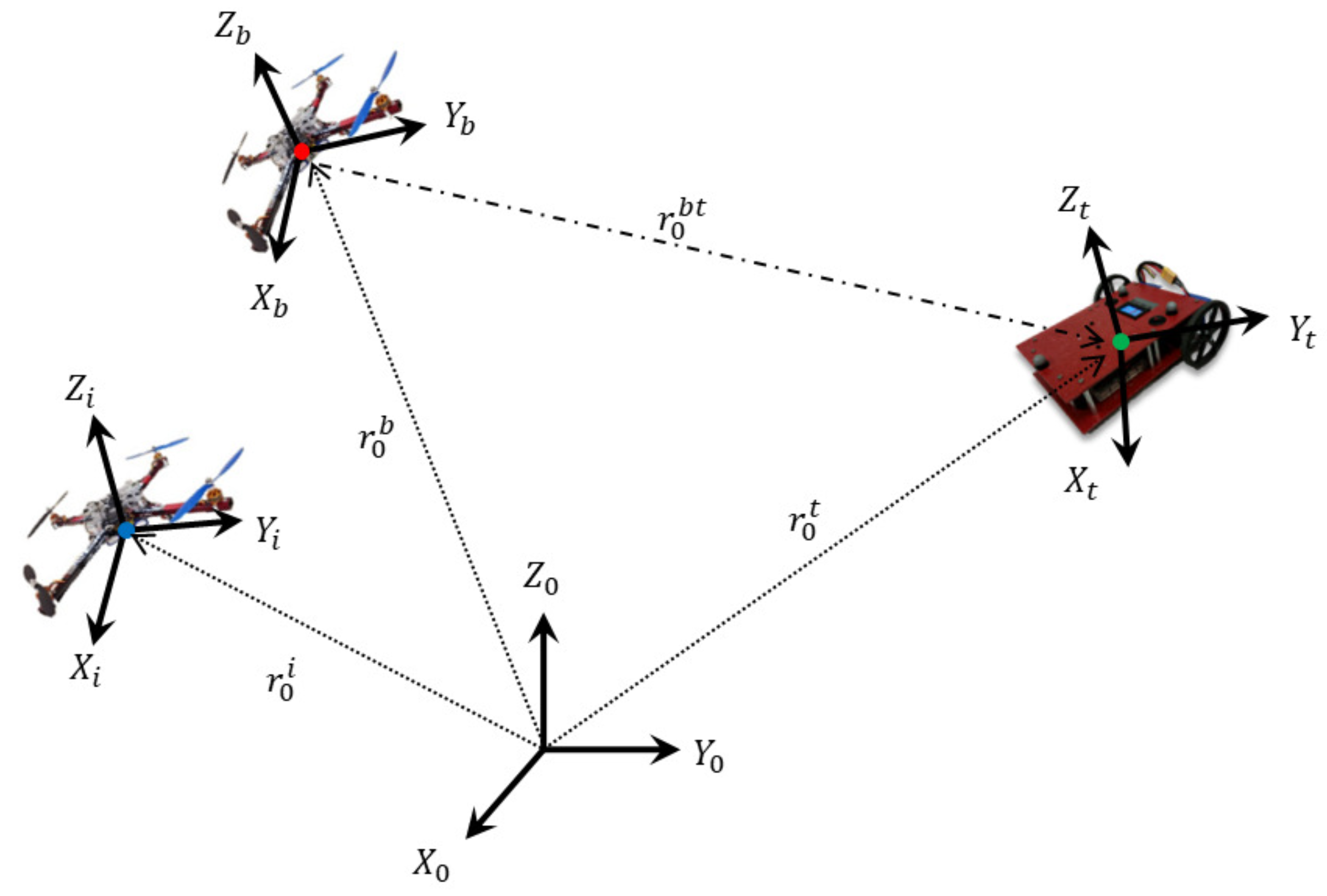
2.1. 3D Vehicle Pose

The body-fixed reference frame $X_v{Y}_v{Z}_v$ is assigned to each vehicle, and its pose is represented by its origin’s position and its orientation with respect to the inertial reference frame $X_0{Y}_0{Z}_0$, as shown for an air vehicle in Figure 1. The position of the vehicle is denoted by the vector $r_0^v={\left[x_0^v{y}_0^v{z}_0^v\right]}^{\top }$, whereas its orientation is determined by the orthogonal rotation matrix $R_0^v$, which maps the coordinates of a vector from $X_v{Y}_v{Z}_v$ to $X_0{Y}_0{Z}_0$. Quaternions are used to compute $R_0^v$ to avoid singularities associated with Euler angles.

The quaternion vector ${\overline{q}}^v$ consists of 4 components:

$${\overline{q}}^v=\left[\begin{array}{c}{q}_0^v\\ q^v\end{array}\right],q^v=\left[\begin{array}{c}{q}_1^v\\ q_2^v\\ q_3^v\end{array}\right].$$

(1)

The quaternions form a unit vector, i.e., ${\overline{q}}^{v^{\top }}{\overline{q}}^v-1=0$, since there are only 3 rotational degrees of freedom. Thus, the vehicle’s pose is represented by 7 components of $r_{0_{}}^v$ and ${\overline{q}}^v$.

Quaternions are not physical parameters to be measured and must be derived from $R_0^v$ [28], which can be constructed using measured variables such as Euler angles. The orthogonal rotation matrix $R_0^v$ in terms of quaternions [34] is defined as

$$R_0^v\left({\overline{q}}^v\right)=[2{\left(q_0^v\right)}^2-1]I_3+2[q^v{q}^{v^{\top }}+q_0^{v}S\left(q^v\right)]$$

(2)

where $I_3$ is the $3\times 3$ identity matrix and $S\left(q^v\right)$ defines a skew-symmetric matrix of a vector such that

$$S\left(q^v\right)=\left[\begin{array}{ccc}0& -q_3^v& q_2^v\\ q_3^v& 0& -q_1^v\\ -q_2^v& q_1^v& 0\end{array}\right]$$

(3)

2.2. 3D Vehicle Velocity

The vehicle’s translational velocity vector ${\dot{r}}_0^v$ in $X_0{Y}_0{Z}_0$ is related to its body-fixed velocities in $X_v{Y}_v{Z}_v$ as

$${\dot{r}}_0^v=R_0^v\left({\overline{q}}^v\right)v^v,v^v\triangleq {\dot{r}}_v^v.$$

(4)

The relationship between the angular velocity vector of the vehicle in $X_v{Y}_v{Z}_v$, ${\omega }^v={\left[{\omega }_x^v{\omega }_y^v{\omega }_z^v\right]}^{\top }$ and the time derivative of the quaternion vector, ${\dot{\overline{q}}}^v$, is given by

$${\dot{\overline{q}}}^v=\frac{1}{2}{G}^{v^{\top }}\left({\overline{q}}^v\right){\omega }^v,G^v\left({\overline{q}}^v\right)=\left[\begin{array}{c}-q^v,q_0^v{I}_3-S\left(q^v\right)\end{array}\right]$$

(5)

The time derivatives of the quaternions are derived from the unit vector constraint as ${\overline{q}}^{v^{\top }}{\dot{\overline{q}}}^v=0$.

2.3. 3D Vehicle State Equations

Using the vehicle pose and velocity equations, the equations of motion of the 3D vehicle are derived as

$$\begin{array}{ccc}\hfill {\dot{v}}^v& =& -S\left({\omega }^v\right)v^v+\frac{F^v}{m^v}\hfill \end{array}$$

(6)

$$\begin{array}{ccc}\hfill {\dot{\omega }}^v& =& -{\left(I^v\right)}^{-1}S\left({\omega }^v\right)I^v{\omega }^v+{\left(I^v\right)}^{-1}{\tau }^v\hfill \end{array}$$

(7)

where $F^v={\left[00F_z^v\right]}^{\top }$ and ${\tau }^v{\left[{\tau }_x^v{\tau }_y^v{\tau }_z^v\right]}^{\top }$ are the input force and moment vectors, respectively, $m^v$ is the mass, and $I^v$ is the $3\times 3$ moment of inertia matrix of the vehicle. Given these equations, the $13\times 1$ state and $6\times 1$ input vectors are defined as

$${\mathsf{x}}^v={\left[\begin{array}{cccc}{r}_0^{v^{\top }}& {\overline{q}}^{v^{\top }}& v^{v^{\top }}& {\omega }^{v^{\top }}\end{array}\right]}^{\top },\mathsf{u}={\left[\begin{array}{cc}{F}^{v^{\top }}& {\tau }^{v^{\top }}\end{array}\right]}^{\top }$$

(8)

The general nonlinear state equations are then given as

$$\dot{\mathsf{x}}=f^v\left({\mathsf{x}}^v\right)+g^v\mathsf{u}$$

(9)

where

$$f^v\left({\mathsf{x}}^v\right)=\left[\begin{array}{c}{R}_0^v\left({\overline{q}}^v\right)v^v\\ \frac{1}{2}{G}^{v^{\top }}\left({\overline{q}}^v\right){\omega }^v\\ -S\left({\omega }^v\right)v^v\\ -I^{v^{-1}}S\left({\omega }^v\right)I^v{\omega }^v\end{array}\right],g^v=\left[\begin{array}{cc}{0}_3& 0_3\\ 0_{4\times 3}& 0_{4\times 3}\\ \frac{1}{m^v}{I}_3& 0_3\\ 0_3& I^{v^{-1}}\end{array}\right]$$

(10)

where $0_3$ and $0_{4\times 3}$ are the $3\times 3$ and $4\times 3$ zero matrices, respectively. Linearization is required for any EKF base-state estimation. The $13\times 13$ Jacobian matrix $J^v$ of the state Equations (8) is derived as

$$J^v={\displaystyle \frac{\partial \left(f^v\left({\mathsf{x}}^v\right)\right)}{\partial {\mathsf{x}}^v}}=\left[\begin{array}{ccccc}{0}_3& \multicolumn{2}{c}{{\displaystyle \frac{\partial {\dot{r}}_0^v}{\partial {\overline{q}}_{}^v}}}& R_0^v\left({\overline{q}}^v\right)& 0_3\\ 0_{4\times 3}& \multicolumn{2}{c}{{\displaystyle \frac{\partial {\dot{\overline{q}}}^v}{\partial {\overline{q}}^v}}}& 0_{4\times 3}& \frac{1}{2}{G}^{v^{\top }}\left({\overline{q}}^v\right)\\ 0_3& \begin{array}{cc}0& 0_3\end{array}& -S\left({\omega }^v\right)& S\left(v^v\right)\\ 0_3& \begin{array}{cc}0& 0_3\end{array}& 0_3& J_{\omega }\end{array}\right]$$

(11)

where $J_{\omega }=I^{v^{-1}}[S\left(I^v{\omega }^v\right)-S\left({\omega }^v\right)I^v]$, and $R_0^v\left({\overline{q}}^v\right)$ and $G^v\left({\overline{q}}^v\right)$ are from (2) and (5), respectively. Given that ${\displaystyle \frac{\partial {\dot{r}}_0^v}{\partial {\overline{q}}^v}}=\left[\begin{array}{cc}{\displaystyle \frac{\partial {\dot{r}}_0^v}{\partial q_0^v}}& {\displaystyle \frac{\partial {\dot{r}}_0^v}{\partial q^v}}\end{array}\right]$, the partial derivatives within the Jacobian matrix are derived as

$$\begin{array}{ccc}\hfill {\displaystyle \frac{\partial {\dot{r}}_0^v}{\partial q_0^v}}& =& {\displaystyle \frac{\partial R{v}^v}{\partial q_0^v}}=[\left(4q_0^v\right)I_3+2S\left(q^v\right)]v^v\hfill \end{array}$$

(12)

$$\begin{array}{ccc}\hfill {\displaystyle \frac{\partial {\dot{r}}_0^v}{\partial q^v}}& =& {\displaystyle \frac{\partial R{v}^v}{\partial q^v}}=2q^v{v}^{v^{\top }}+2\left(q^{v^{\top }}{v}^v\right)I_3-2q_0^{v}S\left(v^v\right)\hfill \end{array}$$

(13)

$$\begin{array}{ccc}\hfill {\displaystyle \frac{\partial {\dot{\overline{q}}}^v}{\partial {\overline{q}}^v}}& =& {\displaystyle \frac{1}{2}}\left[\begin{array}{cc}0& -{\omega }^{v^{\top }}\\ {\omega }^v& -S\left({\omega }^v\right)\end{array}\right]\hfill \end{array}$$

(14)

2.4. Ground Vehicle Model

While our focus in this work is on 3D vehicles, many applications involve networks of ground and air vehicles. Hence, in this section, a model ground vehicles is presented. Figure 1 shows the top view of a ground vehicle’s pose with respect to the inertial reference frame. The pose of a mobile robot is given by its position $(x,y,z$) and its yaw angle $\varphi$. Note that the z component is added since the ground may not be horizontal, and quaternions are not necessary due to a single rotational degree of freedom. Hence, the $7\times 1$ state and $2\times 1$ input vectors for the ground vehicle are defined as

$${\mathsf{x}}^v=\left[\begin{array}{c}{r}_0^v\\ {\varphi }^v\\ v_x^v\\ {\dot{z}}^v\\ {\omega }_z^v\end{array}\right],\mathsf{u}=\left[\begin{array}{c}{F}^v\\ {\tau }^v\end{array}\right]$$

(15)

where $F^v=F_x^v$ and ${\tau }^v={\tau }_z^v$. The components of the state Equations (10) for this ground vehicle model are given as

$$f^v\left({\mathsf{x}}^v\right)=\left[\begin{array}{c}{v}_x^{v}cos\left({\varphi }^v\right)-d^v{\omega }_z^{v}sin\left({\varphi }^v\right)\\ v_x^{v}sin\left({\varphi }^v\right)+d^v{\omega }_z^{v}cos\left({\varphi }^v\right)\\ 0\\ {\omega }_z^v\\ d^v{\left({\omega }_z^v\right)}^2\\ 0\\ -\frac{m^v{d}^v}{I_{zz}^v}{\omega }_z^v{v}_x^v\end{array}\right],g^v=\left[\begin{array}{cc}{0}_{4\times 1}& 0_{4\times 1}\\ 1/m^v& 0\\ 0& 0\\ 0& 1/I_{zz}^v\end{array}\right]$$

(16)

where d is the distance from the rear axle to the vehicle origin. Note that the lateral velocity component is derived based on the mobile robot configuration as $v_y^v=d{\omega }_z^v$ and therefore not included as a state. The Jacobian matrix of the linearized state equations is

$${\displaystyle \frac{\partial \left(f^v\left({\mathsf{x}}^v\right)\right)}{\partial {\mathsf{x}}^v}}=\left[\begin{array}{ccccccc}0& 0& 0& -v_x^{v}sin\left({\varphi }^v\right)-d^v{\omega }_z^{v}cos\left({\varphi }^v\right)& cos\left({\varphi }^v\right)& 0& -d^{v}sin\left({\varphi }^v\right)\\ 0& 0& 0& v_x^{v}cos\left({\varphi }^v\right)-d^v{\omega }_z^{v}sin\left({\varphi }^v\right)& sin\left({\varphi }^v\right)& 0& d^{v}cos\left({\varphi }^v\right)\\ 0& 0& 0& 0& 0& 0& 0\\ 0& 0& 0& 0& 0& 0& 1\\ 0& 0& 0& 0& 0& 0& 2d^v{\omega }_z^v\\ 0& 0& 0& 0& 0& 0& 0\\ 0& 0& 0& 0& -\frac{m^v{d}^v}{I_{zz}^v}{\omega }_z^v& 0& -\frac{m^v{d}^v}{I_{zz}^v}{v}_x^v\end{array}\right]$$

(17)

3. Nonlinear Control Design

Since control design for ground vehicles is trivial and not our focus, we refer the reader to numerous methods, including [35]. Though more recent controllers are available [36], we present a summary of our nonlinear control design for quadcopters [37], for which the control law is derived using Euler angles, noting that conversion of Euler angles to quaternions through the orthogonal rotation matrix is trivial. In this section, we drop the superscript “v” to simplify the notation.

Consider the position vector $r_0^v$ and Euler angle vector $\mathsf{\Phi }={[\varphi ,\theta ,\psi ]}^{\top }$, where $\varphi$, $\theta$, and $\psi$ are the roll, pitch, and yaw angles, respectively. We will treat the quadcopter as a four—input—four—output system with the outputs being $r_0^v$ and $\psi$ and the inputs being the total thrust force $F_z^v=f$ and the three control moments $\tau \equiv {\tau }^v$. In order to derive the nonlinear control law, we divide the system into three subsystems. The first subsystem consists of the roll and pitch moments ${\tau }_x,{\tau }_y$ as the inputs and the $x,y$ components of $r_0^v$ as the outputs. The second subsystem has f as the input and the z component of $r_0^v$ as the output, and the third subsystem has yaw moment ${\tau }_z$ as the input and yaw angle $\psi$ as the output.

3.1. Roll and Pitch Moments

The first subsystem has a relative degree 4, i.e., one must take up to the fourth time derivatives of the outputs $x,y$ to reach the inputs ${\tau }_x,{\tau }_y$. To do this, we use the system model for the translational part of the equations of motion (6) in the earth-fixed frame, which may be written as:

$$\begin{array}{c}\hfill m\ddot{r}=R\left[\begin{array}{c}0\\ 0\\ \widehat{f}\end{array}\right]-\left[\begin{array}{c}0\\ 0\\ mg\end{array}\right]\end{array}$$

(18)

where $R\equiv R_0^v$, g is acceleration due to gravity, and we have replaced the thrust force f with its nominal value $\widehat{f}$. Next, we take the first and second time derivatives of Equation (18):

$$\begin{array}{c}\hfill m\stackrel{⃛}{r}=R\left(\left[\begin{array}{c}0\\ 0\\ \dot{\widehat{f}}\end{array}\right]+\tilde{\omega }\left[\begin{array}{c}0\\ 0\\ \widehat{f}\end{array}\right]\right)\end{array}$$

(19)

$$\begin{array}{c}\hfill m{r}^{\left(4\right)}=R\left(\left[\begin{array}{c}0\\ 0\\ \ddot{\widehat{f}}\end{array}\right]+2\tilde{\omega }\left[\begin{array}{c}0\\ 0\\ \dot{\widehat{f}}\end{array}\right]+(\tilde{\dot{\omega }}+\tilde{\omega }\tilde{\omega })\left[\begin{array}{c}0\\ 0\\ \widehat{f}\end{array}\right]\right)\end{array}$$

(20)

where $\stackrel{⃛}{r}$ and $r^{\left(4\right)}$ are called jerk and snap, respectively. Equation (20) directly relates ${\tau }_x$ and ${\tau }_y$ to snap by substituting for ${\dot{\omega }}_x$ and ${\dot{\omega }}_y$ from (7). Note that ${\dot{\omega }}_z$ and consequently ${\tau }_z$ do not appear in (20).

Next, we define a smooth reference trajectory $r_r={[x_r\left(t\right),y_r\left(t\right),z_r\left(t\right)]}^T$ and the error vector $e_r=r-r_r$ and propose a control law that ensures fourth-order exponentially stable error dynamics with an integral term:

$$\begin{array}{c}\hfill e_r^{\left(4\right)}+5\lambda {\stackrel{⃛}{e}}_r+10{\lambda }^2{\ddot{e}}_r+10{\lambda }^3{\dot{e}}_r+5{\lambda }^4{e}_r\\ \hfill +{\lambda }^5{\int }_0^t{e}_R\left(\sigma \right)d\sigma =0\end{array}$$

(21)

where ${\dot{e}}_r=\dot{r}-V_r$, ${\ddot{e}}_r=\ddot{r}-{\dot{V}}_r$, ${\stackrel{⃛}{e}}_r=\stackrel{⃛}{r}-{\ddot{V}}_r$, $e_r^{\left(4\right)}=r^{\left(4\right)}-{\stackrel{⃛}{V}}_r$, and the integral term is added to reject constant and slowly changing biased (wind) disturbances. For simplicity, the coefficients in the above error dynamics are selected such that all the eigenvalues are at $-\lambda ,\lambda >0$, i.e., the fastest response without oscillations predicted by the model.

Premultiplying Equation (21) by $m{R}^{\top }$, we may write the equation in the following form:

$$\begin{array}{c}\hfill m{R}^{\top }\stackrel{⃛}{V}+5\lambda m{R}^{\top }\ddot{V}+10{\lambda }^{2}m{R}^{\top }\dot{V}+\gamma =0\end{array}$$

(22)

where

$$\begin{array}{c}\gamma =m{R}^{\top }(-{\stackrel{⃛}{V}}_r-5\lambda {\ddot{V}}_r-10{\lambda }^2{\dot{V}}_r+10{\lambda }^3{\dot{e}}_r+5{\lambda }^4{e}_r\hfill \\ \hspace{1em}\hspace{1em}\hspace{1em}\hspace{1em}\hspace{1em}\hspace{1em}\hspace{1em}\hspace{1em}\hspace{1em}\hspace{1em}\hspace{1em}\hspace{1em}\hspace{0.17em}+{\lambda }^5{\int }_0^t{e}_r\left(\sigma \right)d\sigma )\hfill \end{array}$$

(23)

We then substitute from Equations (18)–(20) into Equation (22):

$$\begin{array}{c}\hfill \left[\begin{array}{c}\widehat{f}{\dot{\omega }}_y\\ -\widehat{f}{\dot{\omega }}_x\\ \ddot{\widehat{f}}\end{array}\right]=\left[\begin{array}{c}-2{\omega }_y\\ 2{\omega }_x\\ -5\lambda \end{array}\right]\dot{\widehat{f}}-\left[\begin{array}{c}5\lambda {\omega }_y+{\omega }_z{\omega }_x\\ -5\lambda {\omega }_x+{\omega }_y{\omega }_z\\ 10{\lambda }^2-{\omega }_x^2-{\omega }_y^2\end{array}\right]\widehat{f}\\ \hfill +10{\lambda }^{2}mg\left[\begin{array}{c}{R}_{31}\\ R_{32}\\ R_{33}\end{array}\right]-\gamma \end{array}$$

(24)

where $R_{31}$, $R_{32}$, and $R_{33}$ are the corresponding elements of the rotation matrix R.

Substituting for ${\dot{\omega }}_x$ and ${\dot{\omega }}_y$ from the first two equations of (7) into the first two equations in (24) yields the roll and pitch control moments:

$$\begin{array}{ll}{\tau }_x=& (I_{xx}-I_{yy}+I_{zz}){\omega }_y{\omega }_z-5\lambda I_{xx}{\omega }_x\\ & -\frac{I_{xx}}{\widehat{f}}[2{\omega }_x\dot{\widehat{f}}+10{\lambda }^{2}mg{R}_{32}-{\gamma }_2]\end{array}$$

(25)

$$\begin{array}{ll}{\tau }_y=& (I_{xx}-I_{yy}-I_{zz}){\omega }_z{\omega }_x-5\lambda I_{yy}{\omega }_y\\ & +\frac{I_{yy}}{\widehat{f}}[-2{\omega }_y\dot{\widehat{f}}+10{\lambda }^{2}mg{R}_{31}-{\gamma }_1]\end{array}$$

(26)

where ${\gamma }_1,{\gamma }_2$ are the corresponding elements of vector $\gamma$ in (23), and $\widehat{f}$ and $\dot{\widehat{f}}$ are derived by integrating $\ddot{\widehat{f}}$; from the third row of Equation (24) with the hovering/rest initial conditions $\widehat{f}\left(0\right)=mg$ and $\dot{\widehat{f}}\left(0\right)=0$:

$$\ddot{\widehat{f}}=-5\lambda \dot{\widehat{f}}-(10{\lambda }^2-{\omega }_x^2-{\omega }_y^2)\widehat{f}+10{\lambda }^{2}mg{R}_{33}-{\gamma }_3$$

It must be noted that the system model has allowed us to compute the control laws in (25) and (26) in terms of the system states only: i.e., pose variable (r,$\mathsf{\Phi }$) and body velocities (v,$\omega$). Thus, estimates of higher-order derivatives such as acceleration, jerk, and snap are not required. Only the reference trajectory requires higher-order derivatives and thus must be defined in terms of sufficiently smooth time functions.

3.2. Thrust Force

The thrust control force f appears in the third translational equation of motion and thus has a relative degree of 2. Hence, we define second-order exponentially stable error dynamics with an integral term and both eigenvalues at $-{\lambda }_z,{\lambda }_z>0$:

$$\begin{array}{c}\hfill {\ddot{e}}_Z+3{\lambda }_z{\dot{e}}_Z+3{\lambda }_z^2{e}_Z+{\lambda }_z^3{\int }_0^t{e}_Z\left(\sigma \right)d\sigma =0\end{array}$$

(27)

where $e_Z=z-z_r\left(t\right)$, ${\dot{e}}_Z=\dot{z}-{\dot{z}}_r\left(t\right)$, and ${\ddot{e}}_Z={\ddot{z}}_z-{\ddot{z}}_r\left(t\right)$. The third equation in (18) yields $\ddot{z}=R_{33}f/m-g$. Thus, the thrust force may be derived using Equation (27):

$$\begin{array}{c}\hfill f=\frac{m}{R_{33}}(g+{\ddot{z}}_r-3{\lambda }_z{\dot{e}}_Z-3{\lambda }_z^2{e}_Z-{\lambda }_z^3{\int }_0^t{e}_Z\left(\sigma \right)d\sigma ).\end{array}$$

(28)

3.3. Yaw Control

Since ${\tau }_z$ can be expressed in terms of the second time derivatives of the yaw angle output, we again define second-order exponentially stable error dynamics with an integral term and both eigenvalues at $-{\lambda }_{\psi },{\lambda }_{\psi }>0$:

$$\begin{array}{c}\hfill {\ddot{e}}_{\psi }+3{\lambda }_{\psi }{\dot{e}}_{\psi }+3{\lambda }_{\psi }^2{e}_{\psi }+{\lambda }_{\psi }^3{\int }_0^t{e}_{\psi }\left(\sigma \right)d\sigma =0\end{array}$$

(29)

where $e_{\psi }=\psi -{\psi }_r\left(t\right)$, ${\dot{e}}_{\psi }=\dot{\psi }-{\dot{\psi }}_r\left(t\right)$, ${\ddot{e}}_{\psi }=\ddot{\psi }-{\ddot{\psi }}_r\left(t\right)$, and ${\psi }_r\left(t\right)$ represents the continuously differentiable reference yaw trajectory. We then define the kinematic relationship between angular acceleration ${\dot{\omega }}_z$ and the Euler yaw acceleration $\ddot{\psi }$ as [37]:

$$\begin{array}{c}\hfill \ddot{\psi }=[{\tau }_z-(I_{yy}-I_{xx}){\omega }_x{\omega }_y]/I_{zz}-sin\theta \ddot{\varphi }-cos\theta \dot{\theta }\dot{\psi }.\end{array}$$

(30)

The yaw control moment may then be derived by substituting from (30) into (29):

$$\begin{array}{c}\hfill {\tau }_z=(I_{yy}-I_{xx}){\omega }_x{\omega }_y+I_{zz}[sin\theta \ddot{\varphi }+cos\theta \dot{\theta }\dot{\psi }+{\gamma }_{\varphi }\end{array}$$

(31)

where ${\gamma }_{\varphi }={\ddot{\psi }}_r\left(t\right)-3{\lambda }_{\psi }{\dot{e}}_{\psi }-3{\lambda }_{\psi }^2{e}_{\psi }-{\lambda }_{\psi }^3{\int }_0^t{e}_{\psi }\left(\sigma \right)d\sigma \left)\right]$.

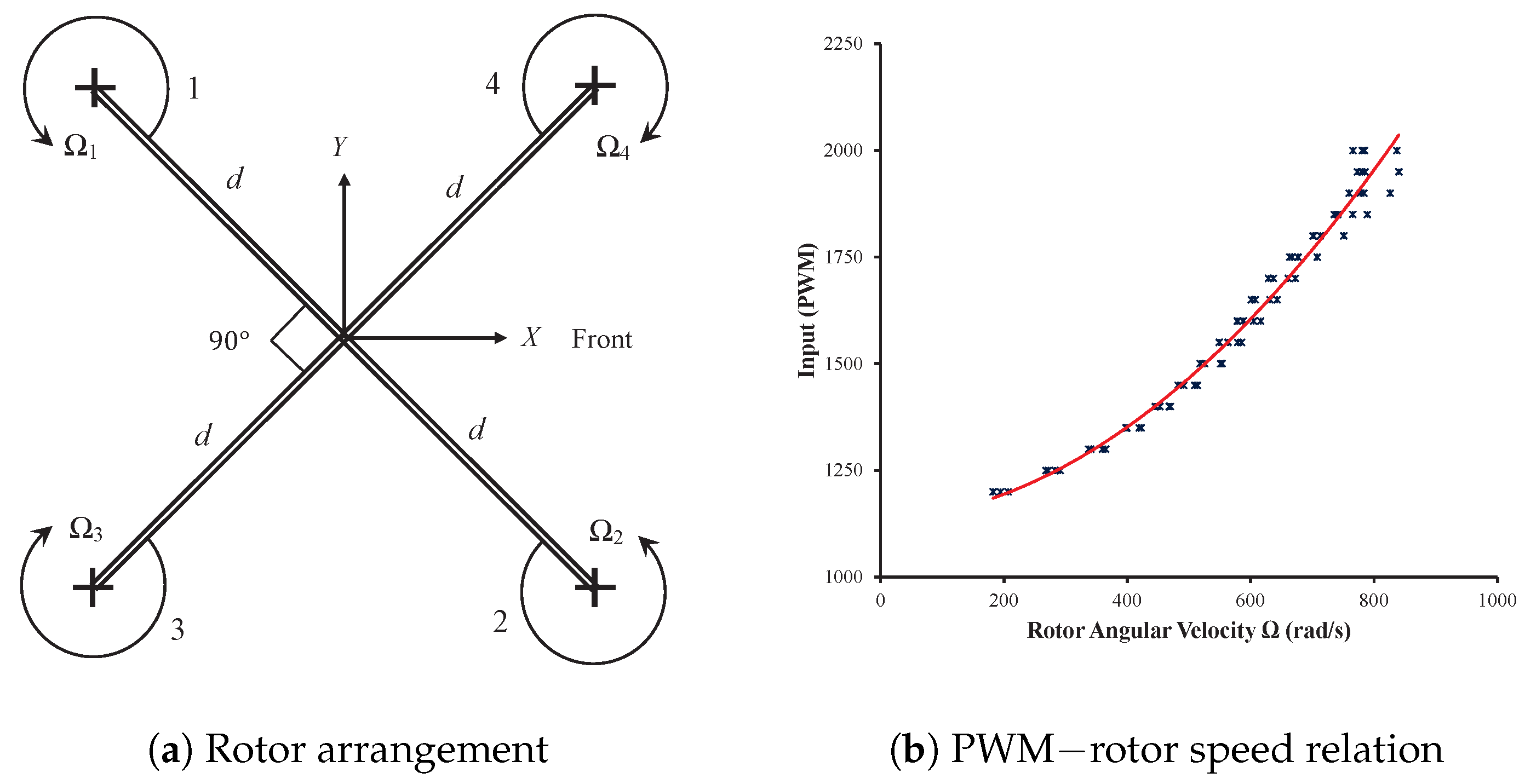
3.4. Relation between Control and Rotor Inputs

The quadrotor motor inputs are expressed in terms of pulse width modulation (PWM) values. Hence, we must relate the four control inputs, total thrust force f, and the three control moments $\tau$ to the motor PWM values. This is done in a two-step process. First, consider the top view of the four rotor arrangements with rotor speeds ${\mathsf{\Omega }}_i,i=1,2,3,4$, as shown in Figure 2a. The control inputs are related to the four input rotor speeds via the following invertible transformation:

$$\begin{array}{c}\hfill \left[\begin{array}{c}f\\ {\tau }_x\\ {\tau }_y\\ {\tau }_z\end{array}\right]=\left[\begin{array}{cccc}{c}_T& c_T& c_T& c_T\\ d{c}_T& -d{c}_T& -d_3{c}_T& d{c}_T\\ d{c}_T& -d{c}_T& d{c}_T& -d{c}_T\\ -c_Q& -c_Q& c_Q& c_Q\end{array}\right]\left[\begin{array}{c}{\mathsf{\Omega }}_1^2\\ {\mathsf{\Omega }}_2^2\\ {\mathsf{\Omega }}_3^2\\ {\mathsf{\Omega }}_4^2\end{array}\right]\end{array}$$

(32)

where d is the arm length and $c_T,C_Q>0$ are the experimentally derived equivalent thrust and torque coefficients. A series of experiments were then performed by applying PWM values and measuring the resulting rotor speeds with a laser tachometer. The resulting data along with the best-fit plot are shown in Figure 2b, and the relationship is given by:

$$\begin{array}{c}\hfill PWM=0.0012{\mathsf{\Omega }}^2+0.0684\mathsf{\Omega }+1132.59\end{array}$$

(33)

4. Multi-Vehicle System Model

The controller presented in the previous section requires state feedback. However, it may be essential not to rely on absolute position feedback from GPS in multi-vehicle systems. Here, we present the case of multi-vehicle systems for which relative position measurements are employed to formulate the cooperative localization algorithm for improved state estimation. We assume that each vehicle possesses an IMU to measure its own orientation fairly accurately, which is a reasonable assumption.

Consider the multi-vehicle system shown in Figure 3. In this system, the base vehicle b can measure the position of the target vehicle t relative to its own body-fixed reference frame. We denote the relative position measurement vector by $\mathsf{z}=\mathsf{r}$, which is given in terms of the system states as:

$$r={R_0^b}^{\top }{r}_0^{bt}={R_0^b}^{\top }(r_0^t-r_0^b)={R_0^b}^{\top }{r}_0$$

(34)

where $r_0=r_0^t-r_0^b$.

The linearized measurement equation is given by $\mathsf{z}=H\mathsf{x}$, where $H=\left[\begin{array}{cc}{H}^b& H^t\end{array}\right]$. The structure and size of this matrix depends on the types of vehicles involved in the measurement. If both the base and target are 3D vehicles, the $3\times 26$ H matrix is given as:

$$H=\left[\begin{array}{ccccc}-{R_0^b}^{\top }& \frac{\mathrm{d}r}{\mathrm{d}{\overline{q}}^b}& 0_{3\times 6}& {R_0^b}^{\top }& 0_{3\times 10}\end{array}\right]$$

(35)

and ${\displaystyle \frac{\mathrm{d}r}{\mathrm{d}{\overline{q}}^b}}=\left[\begin{array}{cc}{\displaystyle \frac{\mathrm{d}r}{\mathrm{d}{q}_0^b}}& {\displaystyle \frac{\mathrm{d}r}{\mathrm{d}{q}^b}}\end{array}\right]$ can be determined using (12):

$$\begin{array}{ccc}\hfill \frac{\mathrm{d}r}{\mathrm{d}{q}_0^b}& =& [\left(4q_0^b\right)I_3+2S\left(q^b\right)]r_0\hfill \end{array}$$

(36)

$$\begin{array}{ccc}\hfill \frac{\mathrm{d}r}{\mathrm{d}{q}^b}& =& 2q^b{r}_0^{\top }+2\left(q^{b^{\top }}{r}_0\right)I_3-2q_0^{b}S\left(r_0\right).\hfill \end{array}$$

(37)

As shown in Figure 3, a network may comprise 2D and 3D vehicles. Since the state vector for 2D vehicles is different, the linearized H matrix will have a different size and components if the base or target is a ground vehicle. When a base ground vehicle measures the relative position of a target ground (target) vehicle, the $3\times 14$ H matrix is defined as

$$H=\left[\begin{array}{ccccc}-{R_0^b}^{\top }& {\displaystyle \frac{\partial r}{\partial {\varphi }^b}}& 0_{3\times 3}& {R_0^b}^{\top }& 0_{3\times 4}\end{array}\right]$$

(38)

where

$${\displaystyle \frac{\partial r}{\partial {\varphi }^b}}=\left[\begin{array}{ccc}-sin{\varphi }^b& cos{\varphi }^b& 0\\ -cos{\varphi }^b& -sin{\varphi }^b& 0\\ 0& 0& 0\end{array}\right]r_0$$

(39)

In cases for which a base ground vehicle measures the relative position of a 3D vehicle, we have

$$H=\left[\begin{array}{ccccc}-{R_0^b}^{\top }& {\displaystyle \frac{\partial r}{\partial {\varphi }^b}}& 0_{3\times 3}& {R_0^b}^{\top }& 0_{3\times 10}\end{array}\right].$$

(40)

Finally, when a base air vehicle measures the relative position of a ground vehicle, we have

$$H=\left[\begin{array}{ccccc}-{R_0^b}^{\top }& {\displaystyle \frac{\partial r}{\partial {\varphi }^b}}& 0_{3\times 6}& {R_0^b}^{\top }& 0_{3\times 4}\end{array}\right].$$

(41)

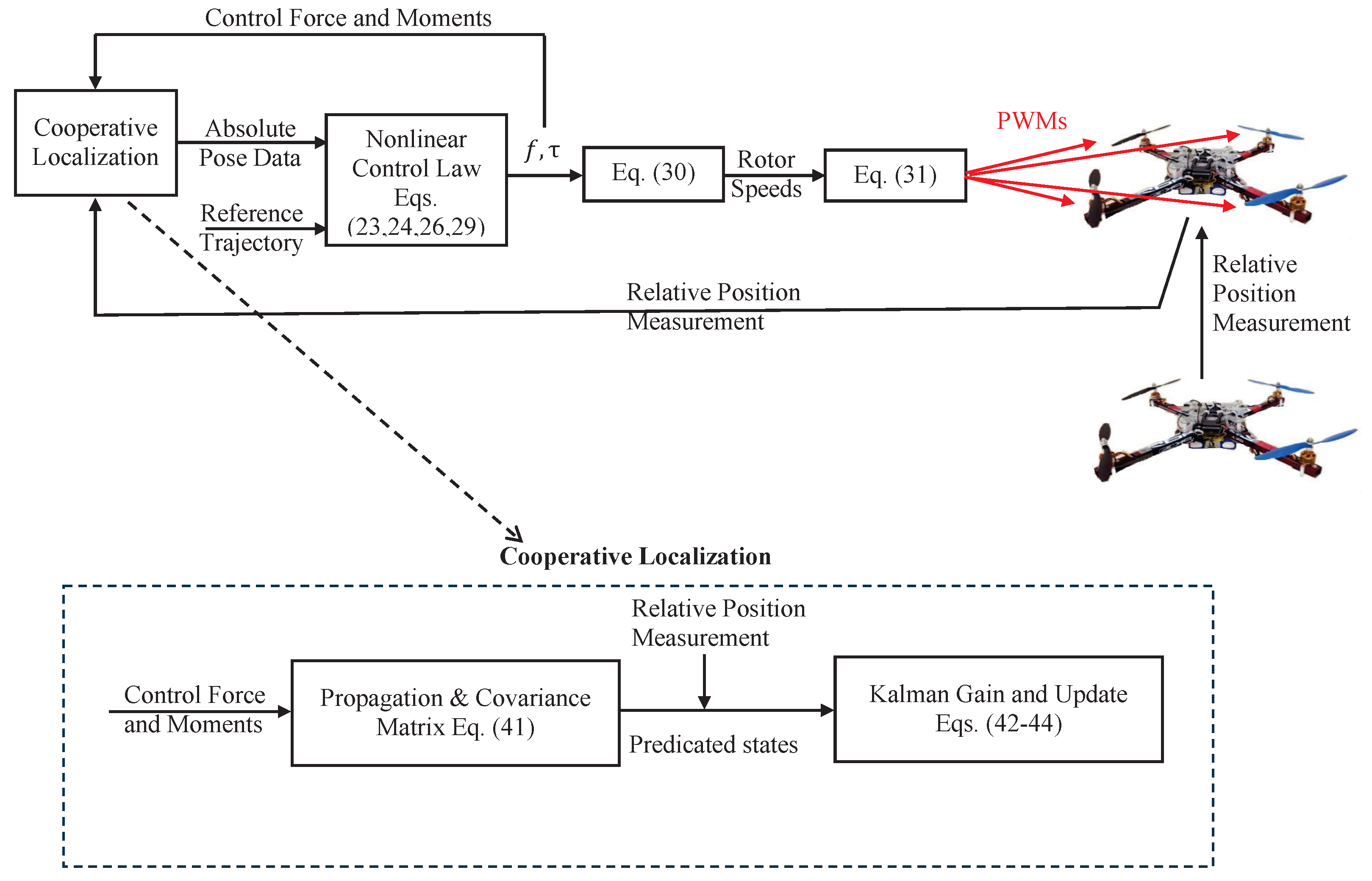
5. Cooperative Localization

Let us consider a system of n vehicles numbered 1 through n. At sample time $\left(k\right)$, a vehicle i uses absolute measurements to propagate its pose using the noisy discrete form of (9) as follows:

$${\mathsf{x}}^i(k+1)=f^i\left({\mathsf{x}}^i\left(k\right)\right)+g^i\left(k\right){\mathsf{u}}^i\left(k\right)+{\gamma }^i\left({\mathsf{x}}^i\left(k\right)\right){\eta }^i\left(k\right)$$

(42)

where ${\mathsf{x}}^i$, ${\mathsf{u}}^i$, and ${\eta }^i$ represent the state, input, and process noise vectors, respectively, and $g^i$ and ${\gamma }^i\left({\mathsf{x}}^i\right)$ are the input and process noise coefficient functions.

Now, let us assume that vehicle i in the set $\{1,\cdots ,n\}$ can take a relative measurement of the pose of a vehicle $j\ne i$. In that case, the measurement vector ${\mathsf{z}}^{ij}$ is given by

$${\mathsf{z}}^{ij}(k+1)=h^{ij}({\mathsf{x}}^i\left(k\right),{\mathsf{x}}^j\left(k\right))+{\nu }^i\left(k\right)$$

(43)

where $h^{ij}$ is defined in (34), and ${\nu }^i\left(k\right)$ represents the measurement noise.

Assuming the initial conditions ${\mathsf{x}}^i\left(0\right)$ and starting with an initial guess $P^i\left(0\right)>0$ with zero cross-covariance, vehicles $i=1,\cdots ,n$ can predict their states by propagation as:

$$\begin{array}{cc}\hfill & {\widehat{\mathsf{x}}}^{i-}(k+1)=f\left({\mathsf{x}}^{i+}\left(k\right)\right)+g^i\left(k\right){\mathsf{u}}^i\left(k\right)\hfill \\ \hfill & P^{i-}(k+1)=J^i\left(k\right)P^{i+}\left(k\right){J^i}^{\top }\left(k\right)+{\mathsf{\Gamma }}_i\left(k\right)Q^i{{\mathsf{\Gamma }}_i}^{\top }\left(k\right),\hfill \\ \hfill & P^{ij-}(k+1)=J^i\left(k\right)P^{i+}\left(k\right){J^j}^{\top }\left(k\right),j=1,\cdots ,n,j\ne i\hfill \end{array}$$

(44)

where $J^i\left(k\right)$ is calculated using (11), $Q^i>0$ is the covariance of the process noise, and ${\mathsf{\Gamma }}^i={\displaystyle \frac{\partial {\gamma }^i}{\partial {\mathsf{x}}^i}}$.

When a “base” vehicle b takes relative measurements of a “target” vehicle t, the innovation error is given by:

$$\begin{array}{cc}\hfill & e^{bt}(k+1)={\mathsf{z}}^{bt}-h^{bt}({\widehat{\mathsf{x}}}^{b-}(k+1),{\widehat{\mathsf{x}}}^{t-}(k+1))\hfill \\ \hfill & \approx {\mathsf{z}}^{bt}-\left[H^b(k+1)H^t(k+1)\right]\left[\begin{array}{c}{\widehat{\mathsf{x}}}^{b-}(k+1)\\ {\widehat{\mathsf{x}}}^{t-}(k+1)\end{array}\right]\hfill \end{array}$$

(45)

where $H^b$ and $H^t$ are defined in (35), (38), (40), or (41) depending on the vehicles involved in the relative measurement. The cross-covariance terms create a slight modification to the innovation covariance matrix:

$$\begin{array}{cc}\hfill S^{bt}& =H^b{P}^{b-}{H^b}^{\top }+H^t{P}^{t-}{H^t}^{\top }\hfill \\ \hfill & +H^b{P}^{bt-}{H^t}^{\top }+H^t{P}^{tb-}{H^b}^{\top }+{\mathcal{R}}^{bt}\hfill \end{array}.$$

(46)

Using (45) and (46), the Kalman gains, states, and covariances for all vehicles $i=1,\cdots ,n$ are updated as:

$$\begin{array}{cc}\hfill & K^i=[P^{it-}{H^t}^{\top }+P^{ib-}{H^b}^{\top }]{S^{bt}}^{-1}\hfill \\ \hfill & {\widehat{\mathsf{x}}}^{i-}={\widehat{\mathsf{x}}}^{i-}+K^i{e}^b\hfill \\ \hfill & P^{i+}=P^{i-}-K^i{S}^{bt}{K^i}^{\top }\hfill \\ \hfill & P^{ij+}=P^{ij-}-K^i{S}^{bt}{K^j}^{\top },j=1,\cdots ,n,j\ne i.\hfill \end{array}$$

(47)

As long as the measurement noise is reasonable and the EKF linearization is accurate, the semi-definite Kalman gain matrix can guarantee a reduction in localization error with every relative measurement. A block diagram of control system implementation with the help of relative measurements and cooperative localization is shown in Figure 4.

6. Results

We have performed a variety of simulations and experiments to verify the CL algorithm’s effectiveness in improving state estimation and closed-loop control performance.

6.1. Experimental Setup

The experiments were performed in a $4.5\mathrm{m}\times 4.0\mathrm{m}\times 3.0\mathrm{m}$ cage with a state-of-the-art vision system capable of 3D localization with sub-millimeter accuracy at 250 frames per second. We formed heterogeneous vehicle networks with small in-house-designed quadcopters and wheeled mobile robots representing ground vehicles.

Figure 5 shows details of one of the quadcopters and mobile robots. The quadcopter components include DJI Flame Wheel Kits with ESC (electronic speed control) motors and propellers, a Raspberry Pi 3 B+ for processing and IO purposes, a PWM driver for the four ESC motors, an OLED display, a 3000 mAh lithium-polymer battery, a voltage measurement unit, and a simple remote relay. They are also equipped with a custom-designed PCB board to simplify the driver and sensor connections and an IMU. The mobile robots are differential-drive with two motors, a dual-motor control, a Raspberry Pi 3 B+, an Arduino Due board, an IMU, and a LiDAR sensor. All vehicles have infrared markers so that their motion can be accurately tracked by the motion-capture system and reported for comparison purposes.

For quadcopters, the control software calculates the three moments and thrust force according to (25)–(28). It then calculates the corresponding rotor speeds and converts the data to PWM motor commands by interpolating a lookup table [37]. For mobile robots, the controller outputs calculate the surge force and yaw moment and then converts them to wheel speeds. These speeds are sent from the Raspberry Pi to an Arduino Due. A fast-rate PI closed-loop control then maintains the commanded wheel speeds for the mobile robot.

We used identical quadcopters and identical mobile robots in our experiments. The mass and geometric properties, which are primarily used for state estimation in CL, are:

$$\begin{array}{ccc}& m& =1.01\mathrm{kg},I=diag(0.0066,0.0065,0.0109)\mathrm{kg}{\mathrm{m}}^2\hfill \\ & d& =0.226\mathrm{m},c_T=7\times {10}^{-6}\mathrm{kgm}{c}_Q=2.6\times {10}^{-7}\mathrm{kg}{\mathrm{m}}^2\mathrm{quadcopters}\hfill \\ & m& =1.748\mathrm{kg},I_{zz}=0.0126\mathrm{kg}{\mathrm{m}}^2,d=0.05\mathrm{m}\mathrm{mobile}\mathrm{robots}\hfill \end{array}$$

The measurements were all take at 50 Hz, i.e., $\mathsf{\Delta }t=0.02\mathrm{s}$. Meanwhile, the same rate was selected for propagation of the state equations for CL. We assumed a standard deviation of $0.005\mathrm{m}$ for all position-state measurements and 0.1${}^{\circ }$ for all orientation-state measurements. We also assumed the process noise covariance matrix to be diagonal, with $0.1$ values as diagonal elements.

6.2. Validation Results

We initially conducted a series of experiment designed to validate the CL algorithm. In these experiments, the closed-loop control algorithm was implemented without the use of the CL algorithm in real time. Instead, the control signals were collected and applied as inputs to the vehicle simulation models with CL. The simulation results were then compared with the recorded motion-capture system data to evaluate the CL algorithm performance.

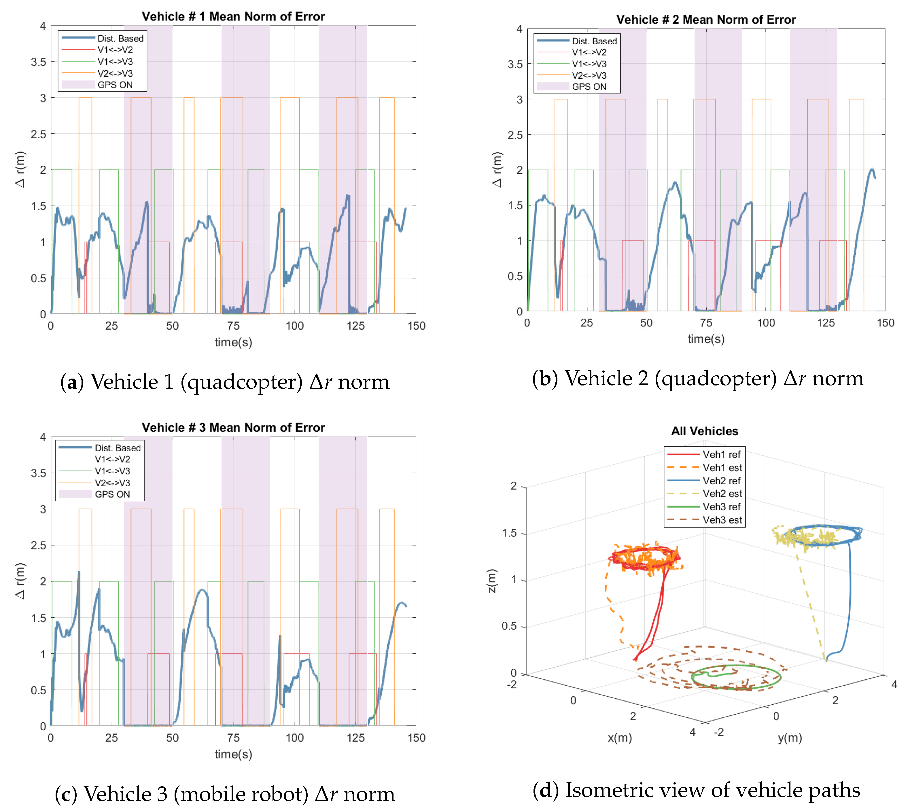
6.2.1. Results with Distance-Based Measurements

We initially considered a three-vehicle network consisting of two quadcopters (Vehicles 1 and 2) and a mobile robot (Vehicle 3). All three vehicles were directed to follow predetermined circular paths using the control algorithm, as shown in Figure 6c. In order to test the CL algorithm, we assumed Vehicle 3 has continuous access to its own absolute position and that relative measurements depend on the proximity of the vehicles. Specifically, the quadcopters (Vehicles 1 and 2) can measure their relative positions when within 4 m of each other and the relative position of the mobile robot (Vehicle 3) when it is a within a 2 m distance.

The estimation error results are shown in Figure 6a,b in the form of the time history of the position-error norms for Vehicles 1 and 2. The estimation error for Vehicle 3 stays relatively small due to consistent availability of the absolute position measurements and therefore is uneventful and is not shown. In the figures, the actual error is identified as “Dist. Based”. Three flags of magnitudes $1,2,$ and 3, are used to distinguish when relative measurements between Vehicles 1 and 2, 1 and 3, and 2 and 3, respectively, are active. The figure illustrates that when the distance between the mobile robot and each quadcopter is within the threshold (i.e., Flags 1 and 2), there is a sharp drop in the position error of the quadcopters. In addition, the relative measurements between the two quadcopters can significantly improve localization if one has access to Vehicle 3. For instance, in Figure 6b at 40 s, Vehicle 2 does not have access to Vehicle 3, but its estimation error drops near zero due to relative measurement between Vehicles 1 and 2 (red line) and Vehicles 1 and 3 (green line). The isometric and top views of the reference (ref) and CL-estimated (est) paths of the three vehicles are presented in Figure 6c,d. These figures demonstrate significant variations to quadcopter localization whenever they do not have any direct or indirect access to the mobile robot (Vehicle 3), which has access to absolute measurements.

Next, we consider the same scenario only now with the mobile robot having intermittent access to its absolute position (simulating occasionally available GPS). We assume continuous “GPS” access for Vehicle 1 for only 20s intervals starting at 30 s, 70 s, and 110 s. This intermittent access is a more realistic representation and shows how this sparsity will affect the overall network localization. Figure 7a–c show the position error norms for Vehicles 1–3, respectively, with shaded areas representing access to GPS. We can make the same conclusions as for the previous case, indicating that even when GPS is sparsely available, it is still beneficial to the vehicles in the network. For example, this can be observed in sharp error drops for Vehicle 2’s position error in Figure 7b at about 30 s, 70 s, 90 s, and 120 s when there are relative measurements of Vehicle 3 available and Vehicle 3 has access to GPS. However, another important conclusion is the significance of relative measurements for absolute localization in the absence of any absolute measurements. For instance, Figure 7a–c show that the localization errors are significantly reduced at 15 s and 90 s for all three vehicles due to relative measurements only since there is no access to GPS by Vehicle 1.

6.2.2. Double-Caravan Measurement Formation

Next, we experimented with a much larger network of eight vehicles in a double-caravan measurement configuration. Each caravan was structured with a“leader” quadcopter vehicle and three mobile robot “followers” such that each vehicle can measure the relative position of its lead vehicle. We numbered the vehicles such that Vehicles 1–3 and 5–7 are mobile robots and Vehicles 4 and 8 are quadcopters. In this scenario, we assume Vehicles 1, 2, 3, 5, 6, and 7 can only measure the relative positions of Vehicles 2, 3, 4, 6, 7, and 8, respectively. Meanwhile, the lead quadcopters (i.e., Vehicles 4 and 8) may or may not have access to GPS. Similar to the previous network, all eight vehicles were directed to follow predetermined circular paths using the control algorithm.

To facilitate information exchange across caravan formations, a specific role is assigned to the two follower Vehicles 1 and 5 (mobile robots) and next to the two lead Vehicles 4 and 8 (quadcopters). These designated “communication” vehicles possess the capacity to access and retrieve the relative position data of one another. This strategic assignment serves as the linchpin for the seamless propagation of cross-covariance and localization information across all vehicles within the caravans. Notably, this operational paradigm is achieved despite communication being primarily limited to the pairing of just two vehicles from each respective caravan formation.

We consider four slightly different measurement cases for this formation, listed in

Table 1. Simultaneous measurement descriptions for double—caravan measurement cases.

	Simultaneous Measurements ($\mathit{b}\to \mathit{t}$)
Case 1	1 → 2, 2 → 3, 3 → 4, 5 → 6, 6 → 7, 7 → 8, 1 → 5
Case 2	1 → 2, 2 → 3, 3 → 4, 5 → 6, 6 → 7, 7 → 8, 1 → 5, 4 → 4 (continuous)
Case 3	1 → 2, 2 → 3, 3 → 4, 5 → 6, 6 → 7, 7 → 8, 1 → 5, 4 → 4 (intermittent)
Case 4	1 → 2, 2 → 3, 3 → 4, 5 → 6, 6 → 7, 7 → 8, 4 → 8

, to evaluate the CL algorithm’s performance. In Cases 1 through 3, Vehicle 1 measures the relative position of Vehicle 5 of the second caravan. In Case 1, there are only relative measurements. In Cases 2 and 3, in addition to the relative measurements, the lead quadcopter of the first caravan, Vehicle 4, has continuous or intermittent absolute position measurement access, respectively. The intermittent access to the absolute position for Vehicle 4 is provided after the first 40s and for 40s duration and then alternates regularly. Finally, in Case 4, there are again only relative measurements, as only the lead quadcopter of the first caravan, Vehicle 4, can measure the relative position of the lead quadcopter, Vehicle 8, of the second caravan.

The position error norms for all vehicles are presented in Figure 8 for Vehicles 1–4 and Figure 9 for Vehicles 5–8. As expected, Case 2 provides the most promising results, with little estimation errors since one vehicle in the network has continuous access to its absolute position and there is a measurement/communication path from the rest of the network to that vehicle. The errors for Cases 1 and 4 have a similar pattern of increasing with time since there are no absolute measurements. However, Case 1 performs slightly better throughout the simulations of all vehicles, indicating that communication and relative measurements between two follower vehicles may be slightly more beneficial than between lead vehicles. In addition, Case 4 consistently results in noisier estimations. Finally, Case 3 demonstrates that even intermittent access to absolute measurements (e.g., GPS) by one vehicle results in full recovery of estimation errors by all vehicles. This is the inherent advantage of CL and results from cross-covariance terms in the covariance matrix.

The isometric views of the reference (ref) and estimated (est) paths and estimated paths of all vehicles for Cases 1 through 4 are shown in Figure 10. It can be clearly seen that both continuous and intermittent access to absolute measurements (e.g., GPS) by one vehicle results in excellent estimation.

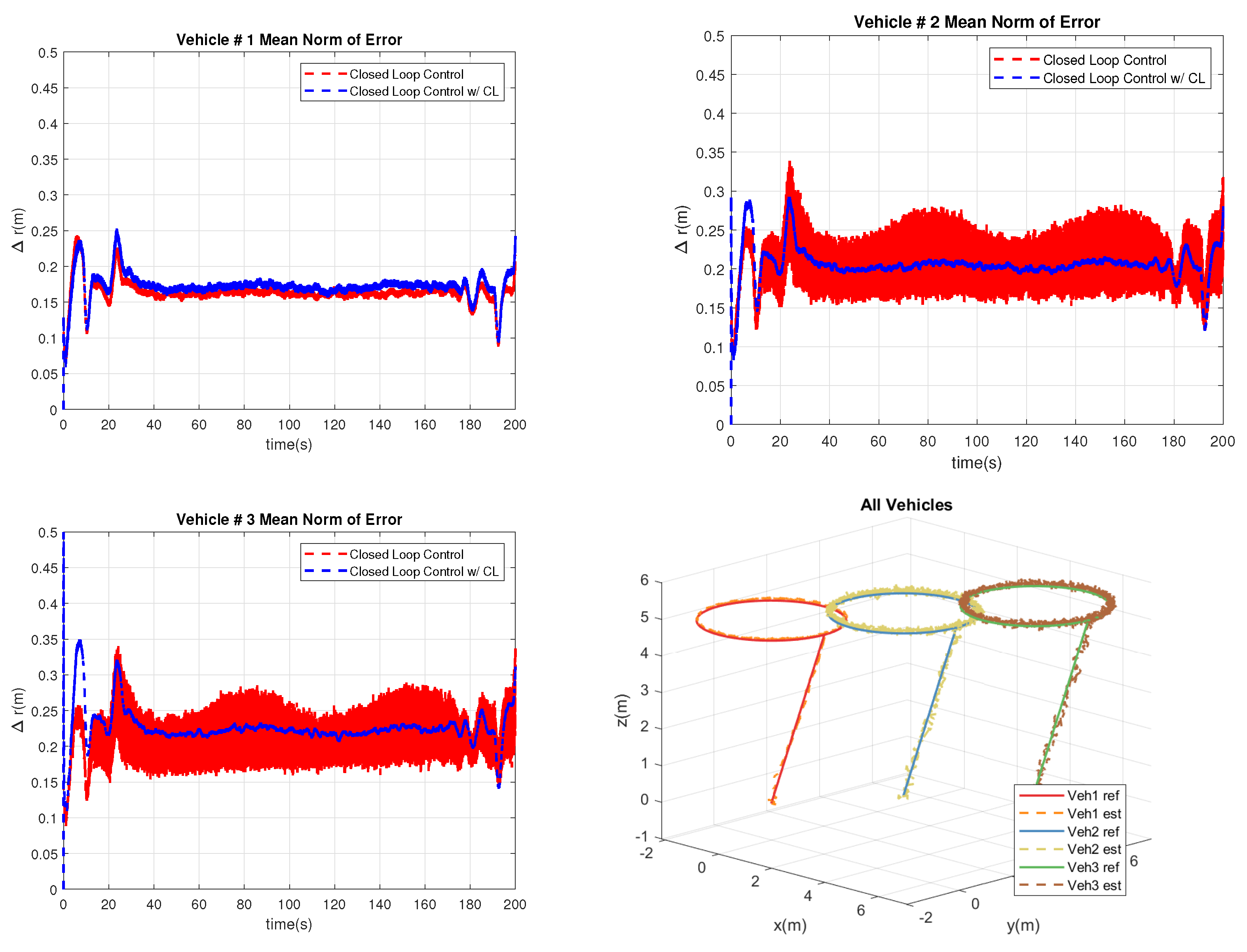
6.3. Closed-Loop Control Results

The final and most significant results of this work involve the application of the nonlinear closed-loop control presented in Section 3 to a network of three vehicles similar to Section 6.2 and a double-caravan network similar to Section 6.2.2.

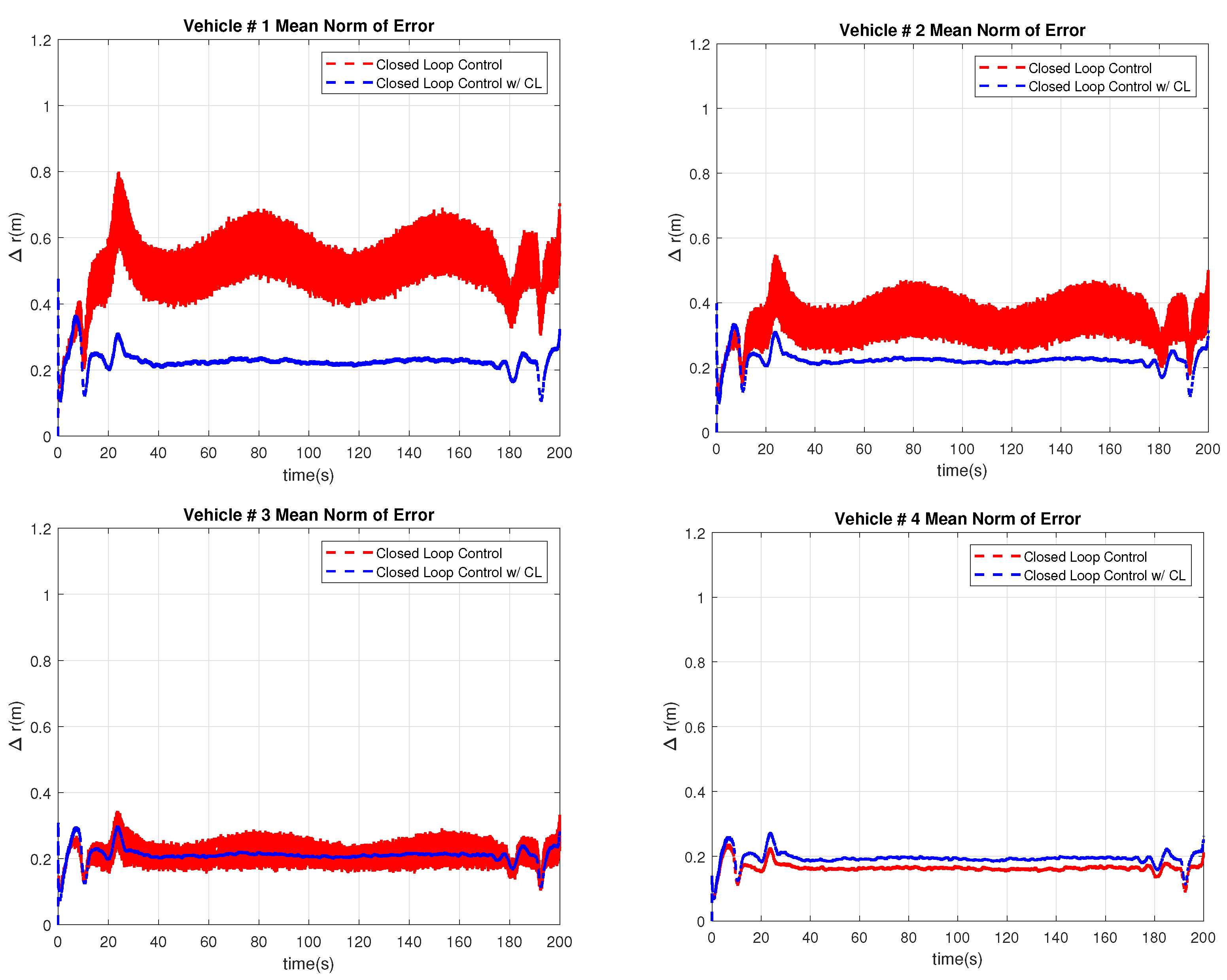
6.3.1. Control of Three-Vehicle Network

First, we consider a three-vehicle network wherein all three vehicles are quadcopters. The vehicles initially lift off to a certain height and then follow predetermined circular paths using the closed-loop control algorithm presented in Section 3: once without and another time with the aid of the CL algorithm. In this scenario, Vehicle 1 is capable of continuously measuring its own absolute position, while Vehicles 2 and 3 exclusively receive relative position measurements from Vehicle 1.

Figure 11 illustrates the position error norms $\mathsf{\Delta }r$ and paths of Vehicles 1 through 3 to compare the performance of the closed-loop control algorithm with and without the aid of CL. The results are promising for both the closed-loop control algorithm and its integration with cooperative localization. There are two important observations. First, the use of CL in state estimation results in significantly reducing the noise in the response and thus significantly reduces the control effort to combat the resulting high-frequency oscillations. The second observation is that there is actually a slight increase in the error for the vehicle that has access to its own absolute measurements: i.e., Vehicle 1.

6.3.2. Control of Double-Caravan Formation

Consider the double—caravan arrangement as in Section 6.2.2 but with all eight vehicles being quadcopters. We consider two cases with the same relative measurement scenario as listed in

Table 2. Simultaneous measurement descriptions for double—caravan formation in closed—loop control.

	Simultaneous Measurements ($\mathit{b}\to \mathit{t}$)
Case 1	1 → 2, 2 → 3, 3 → 4, 5 → 6, 6 → 7, 7 → 8, 8 → 4, 4 → 4 (continuous)
Case 2	1 → 2, 2 → 3, 3 → 4, 5 → 6, 6 → 7, 7 → 8, 8 → 4, 4 → 4 (intermittent)

. In other words, Vehicles 1, 2, 3, 5, 6, 7, and 8 measure the relative positions of Vehicles 2, 3, 4, 6, 7, 8, and 4, respectively. Meanwhile, the leader Vehicle 4 can either continuously measure its own absolute position (Case 1) or can do so intermittently (Case 2).

In these simulations, we explore two cases. In Case 1, Vehicle 4 receives persistent and uninterrupted access to GPS data. In contrast, Case 2 introduces intermittent GPS access for Vehicle 4 with predefined 40s intervals. These experimental modifications will help investigate the implications of consistent versus sporadic GPS availability on the overall system performance, specifically when nonlinear control is present.

Figure 12 and Figure 13 present the time history of the position error norms for Vehicles 1–4 and for Vehicles 5–8, respectively, for Case 1. As in the previous network, Vehicle 4 being able to measure its own absolute position does not benefit from CL, and, in fact, its tracking error slightly increases. Moreover, similar to the previous network, cooperative localization significantly reduces the state estimation noise for all other vehicles. Another interesting phenomenon is that as we go farther away from Vehicle 4, the superiority of CL in reducing the estimation error becomes more apparent, such that Vehicles 1 and 5 see the most benefit, followed by vehicles 2 and 6.

Case 2 is similar to Case 1 except that Vehicle 4 has intermittent access to its own absolute position measurements. We ensured that the vehicle alternates between 40 s of access to its absolute position measurements followed by lack of access for another 40 s. Figure 14 and Figure 15 present the time history of the position error norms for Vehicles 1–4 and 5–8, respectively, for Case 2. The purple bands represent the “GPS” access afforded to Vehicle 4, and the blank spaces in between represent the “GPS” outages. In this case, we can make similar conclusions as those of Case 1: Vehicle 4 having access to its own absolute measurements does not benefit from CL, the noise in state estimation is significantly reduced for all other vehicles, and the benefit of using CL becomes more pronounced as we go down the network from the lead vehicle with absolute measurement. In addition, any time Vehicle 4 has access to its own absolute position, there is significant reduction in position errors whether CL is employed or not.

7. Conclusions

We presented the nonlinear state and relative measurement equations and their linearized forms for networks of 3D and 2D vehicles and implemented a centralized EKF-based CL algorithm for such networks. An exponentially stable closed-loop nonlinear control was presented that required state estimation for feedback. We dove into the synergistic relationship between CL and closed-loop control within vehicle networks and explored the impact of cooperative localization with consistent and intermittent GPS access. After considering both small and large vehicle networks, we have concluded that cooperative localization can significantly improve the performance of closed-loop control in terms of both noise and error reduction for all vehicles that do not have access to their own absolute position measurement, with the former reducing control effort and the latter helping with position accuracy. Furthermore, the reduction in error becomes more significant as we go down the communication link. Finally, we concluded that cooperative localization is not useful for vehicles that have direct access to their own absolute position measurements through, for example, GPS. Hence, we suggest not updating the position of such vehicles with cooperative localization when implementing the algorithm. These findings have further illuminated the intricate dynamics of cooperative localization and closed-loop control, contributing to a comprehensive understanding of their practical implications and the optimal strategies for deployment in diverse vehicle networks.

References

1. Kia, S.S.; Rounds, S.; Martinez, S. Cooperative Localization for Mobile Agents: A Recursive Decentralized Algorithm Based on Kalman-Filter Decoupling. IEEE Control Syst. Mag. 2016, 36, 86–101. [Google Scholar] [CrossRef]
2. Gamini Dissanayake, M.W.M.; Newman, P.; Clark, S.; Durrant-Whyte, H.F.; Csorba, M. A solution to the simultaneous localization and map building (SLAM) problem. IEEE Trans. Robot. Autom. 2001, 17, 229–241. [Google Scholar] [CrossRef]
3. Bibuli, M.; Bruzzone, G.; Caccia, M.; Gasparri, A.; Priolo, A.; Zereik, E. Swarm-based path-following for cooperative unmanned surface vehicles. Proc. Inst. Mech. Eng. Part M J. Eng. Marit. Environ. 2014, 228, 192–207. [Google Scholar] [CrossRef]
4. Liu, K.; Yang, P.; Jiao, L.; Wang, R.; Yuan, Z.; Dong, S. Antisaturation fixed-time attitude tracking control based low-computation learning for uncertain quadrotor UAVs with external disturbances. Aerosp. Sci. Technol. 2023, 142, 108668. [Google Scholar] [CrossRef]
5. Roumeliotis, S.I.; Bekey, G.A. Distributed multirobot localization. IEEE Trans. Robot. Autom. 2002, 18, 781–795. [Google Scholar] [CrossRef]
6. Mayle, M.N.; Sharma, R. Cooperative Localization in a GPS-Limited Environment Using Inter-Vehicle Range Measurements for a System of Multiple, Non-Homogeneous Vehicles. In Proceedings of the AIAA Scitech 2021 Forum, Virtual Event, 11–15, 19–21 January 2021; American Institute of Aeronautics and Astronautics Inc.: Reston, VA, USA, 2021; pp. 1–18. [Google Scholar] [CrossRef]
7. Panzieri, S.; Pascucci, F.; Sciavicco, L.; Setola, R. Distributed multi-robot localization. Robot. Concepts Methodol. Tools Appl. 2013, 1, 391–406. [Google Scholar] [CrossRef]
8. Carrillo-Arce, L.C.; Nerurkar, E.D.; Gordillo, J.L.; Roumeliotis, S.I. Decentralized multi-robot cooperative localization using covariance intersection. In Proceedings of the 2013 IEEE/RSJ International Conference on Intelligent Robots and Systems, Tokyo, Japan, 3–7 November 2013; pp. 1412–1417. [Google Scholar] [CrossRef]
9. Wanasinghe, T.R.; Mann, G.K.I.; Gosine, R.G. Decentralized Cooperative Localization Approach for Autonomous Multirobot Systems. J. Robot. 2016, 2016, 2560573. [Google Scholar] [CrossRef]
10. Nerurkar, E.D.; Roumeliotis, S.I. Asynchronous multi-centralized cooperative localization. In Proceedings of the IEEE/RSJ 2010 International Conference on Intelligent Robots and Systems, IROS 2010—Conference Proceedings, Taipei, Taiwan, 18–22 October 2010; pp. 4352–4359. [Google Scholar] [CrossRef]
11. Zhu, J.; Kia, S.S. Decentralized Cooperative Localization with LoS and NLoS UWB Inter-Agent Ranging. IEEE Sens. J. 2022, 22, 5447–5456. [Google Scholar] [CrossRef]
12. Zhu, P.; Geneva, P.; Ren, W.; Huang, G. Distributed Visual-Inertial Cooperative Localization. In Proceedings of the IEEE International Conference on Intelligent Robots and Systems, Prague, Czech Republic, 27 September–1 October 2021; Institute of Electrical and Electronics Engineers Inc.: Piscataway, NJ, USA, 2021; pp. 8714–8721. [Google Scholar] [CrossRef]
13. Wang, D.; Qi, H.; Lian, B.; Liu, Y.; Song, H. Resilient Decentralized Cooperative Localization for Multisource Multirobot System. IEEE Trans. Instrum. Meas. 2023, 72, 1–13. [Google Scholar] [CrossRef]
14. Liu, Y.; Wang, Y.; Shen, Y.; Shi, X. Hybrid TOA-AOA WLS Estimator for Aircraft Network Decentralized Cooperative Localization. IEEE Trans. Veh. Technol. 2023, 72, 9670–9675. [Google Scholar] [CrossRef]
15. Kia, S.S.; Hechtbauer, J.; Gogokhiya, D.; Martinez, S. Server-Assisted Distributed Cooperative Localization over Unreliable Communication Links. IEEE Trans. Robot. 2018, 34, 1392–1399. [Google Scholar] [CrossRef]
16. Wang, L.; Zhang, T.; Gao, F. Distributed cooperative localization with lower communication path requirements. Robot. Auton. Syst. 2015, 79, 26–39. [Google Scholar] [CrossRef]
17. Wang, X.; Guo, Y.; Cao, J.; Wu, M.; Sun, Z.; Lv, C. Simplify Belief Propagation and Variation Expectation Maximization for Distributed Cooperative Localization. Appl. Sci. 2022, 12, 3851. [Google Scholar] [CrossRef]
18. Huang, Y.; Xue, C.; Zhu, F.; Wang, W.; Zhang, Y.; Chambers, J.A. Adaptive Recursive Decentralized Cooperative Localization for Multirobot Systems with Time-Varying Measurement Accuracy. IEEE Trans. Instrum. Meas. 2021, 70, 1–25. [Google Scholar] [CrossRef]
19. Xin, J.; Xie, G.; Yan, B.; Shan, M.; Li, P.; Gao, K. Multimobile Robot Cooperative Localization Using Ultrawideband Sensor and GPU Acceleration. IEEE Trans. Autom. Sci. Eng. 2022, 19, 2699–2710. [Google Scholar] [CrossRef]
20. Lin, J.; Lou, Z.; Zweigel, R.; Abel, D. Cooperative Localization of a Networked Multi-Vehicle System. IFAC-PapersOnLine 2019, 52, 67–72. [Google Scholar] [CrossRef]
21. Wu, Y.; Peng, B.; Wymeersch, H.; Seco-Granados, G.; Kakkavas, A.; Garcia, M.H.C.; Stirling-Gallacher, R.A.; Casta, M.H.; Stirling-Gallacher, R.A. Cooperative Localization with Angular Measurements and Posterior Linearization. In Proceedings of the 2020 IEEE International Conference on Communications Workshops (ICC Workshops), Dublin, Ireland, 7–11 June 2020; pp. 1–6. [Google Scholar] [CrossRef]
22. Qu, M.; Lu, H. Cooperative Simultaneous Localization and Mapping with Local Measurements in 2D Space. In Proceedings of the 2021 6th International Conference on Automation, Control and Robotics Engineering (CACRE), Dalian, China, 15–17 July 2021; pp. 509–513. [Google Scholar] [CrossRef]
23. Han, Y.; Wei, C.; Li, R.; Wang, J.; Yu, H. A novel cooperative localization method based on IMU and UWB. Sensors 2020, 20, 467. [Google Scholar] [CrossRef]
24. Héry, E.; Xu, P.; Bonnifait, P.; Hery, E.; Xu, P.; Bonnifait, P. Consistent decentralized cooperative localization for autonomous vehicles using LiDAR, GNSS, and HD maps. J. Field Robot. 2021, 38, 552–571. [Google Scholar] [CrossRef]
25. Pires, A.G.; Rezeck, P.A.F.; Chaves, R.A.; Macharet, D.G.; Chaimowicz, L. Cooperative Localization and Mapping with Robotic Swarms. J. Intell. Robot. Syst. Theory Appl. 2021, 102, 1–23. [Google Scholar] [CrossRef]
26. Ben, Y.; Sun, Y.; Li, Q.; Cui, W.; Zhang, Q. A Cooperative Localization Algorithm Considering Unknown Ocean Currents for Multiple AUVs. In Lecture Notes in Electrical Engineering; Springer Science and Business Media Deutschland GmbH: Singapore, 2022; Volume 861, pp. 1379–1387. [Google Scholar]
27. Shan, X.; Cabani, A.; Chafouk, H. Cooperative Localization Based on GPS Correction and EKF in Urban Environment. In Proceedings of the 2022 2nd International Conference on Innovative Research in Applied Science, Engineering and Technology, IRASET 2022, Meknes, Morocco, 3–4 March 2022; Institute of Electrical and Electronics Engineers Inc.: Piscataway, NJ, USA, 2022. [Google Scholar] [CrossRef]
28. Oliveros, J.C.; Ashrafiuon, H. Application and Assessment of Cooperative Localization in Three-Dimensional Vehicle Networks. Appl. Sci. 2022, 12, 11805. [Google Scholar] [CrossRef]
29. Oliveros, J.C.; Ashrafiuon, H. Cooperative Localization Using the 3D Euler–Lagrange Vehicle Model. Guid. Navig. Control 2022, 2, 2250018. [Google Scholar] [CrossRef]
30. Miller, A.; Rim, K.; Chopra, P.; Kelkar, P.; Likhachev, M. Cooperative Perception and Localization for Cooperative Driving. In Proceedings of the IEEE International Conference on Robotics and Automation, Paris, France, 31 May–31 August 2020; Institute of Electrical and Electronics Engineers Inc.: Piscataway, NJ, USA, 2020; pp. 1256–1262. [Google Scholar] [CrossRef]
31. Ilaya, O. Cooperative Control for Multi-Vehicle Swarms. Ph.D. Thesis, RMIT University, Melbourne, Australia, 2009. [Google Scholar]
32. Yin, T.; Zou, D.; Lu, X.; Bi, C. A Multisensor Fusion-Based Cooperative Localization Scheme in Vehicle Networks. Electronics 2022, 11, 603. [Google Scholar] [CrossRef]
33. Ren, W.; Beard, R.W. Distributed consensus in multi-vehicle cooperative control: Theory and applications. In Communications and Control Engineering; Number 9781848000148 in Communications and Control Engineering; Springer: London, UK, 2008; pp. 1–315. [Google Scholar] [CrossRef]
34. Betsch, P.; Siebert, R. Rigid body dynamics in terms of quaternions: Hamiltonian formulation and conserving numerical integration. Int. J. Numer. Methods Eng. 2009, 79, 444–473. [Google Scholar] [CrossRef]
35. Ashrafiuon, H.; Nersesov, S.; Clayton, G. Trajectory Tracking Control of Planar Underactuated Vehicles. IEEE Trans. Autom. Control 2017, 62, 1959–1965. [Google Scholar] [CrossRef]
36. Tang, P.; Lin, D.; Zheng, D.; Fan, S.; Ye, J. Observer based finite-time fault tolerant quadrotor attitude control with actuator faults. Aerosp. Sci. Technol. 2020, 104, 105968. [Google Scholar] [CrossRef]
37. Poultney, A.; Kennedy, C.; Clayton, G.; Ashrafiuon, H. Robust Tracking Control of Quadrotors Based on Differential Flatness: Simulations and Experiments. IEEE/ASME Trans. Mechatron. 2018, 23, 1126–1137. [Google Scholar] [CrossRef]
Figure 1. Kinematic models for 3D air vehicles (a) and 2D ground vehicles (b).
Electronics 12 04945 g001
Figure 2. (a) Top view of the quadrotor model; (b) PWM vs. rotor speed and its best fit model in red.
Electronics 12 04945 g002
Figure 3. Absolute and relative pose geometry.
Electronics 12 04945 g003
Figure 4. Block diagram of control system implementation with the help of cooperative localization.
Electronics 12 04945 g004
Figure 5. The experimental in-house quadcopter (a) and ground vehicle (b).
Electronics 12 04945 g005
Figure 6. Three—vehicle test case with distance—based relative measurements: error norm and measurement flags for Vehicle 1 (a); error norm and measurement flags for Vehicle 2 (b); estimated versus actual paths: isometric view (c) and top view (d).
Electronics 12 04945 g006
Figure 7. Three—vehicle test case with distance—based relative measurements and intermittent Vehicle 1 GPS access: error norm and measurement flags for Vehicle 1 (a); error norm and measurement flags for Vehicle 2 (b); estimated versus actual paths: isometric view (c) and top view (d).
Electronics 12 04945 g007
Figure 8. Position error norms of Vehicles 1–4 for the four measurement cases of double-caravan experiment.
Electronics 12 04945 g008
Figure 9. Position error norms of Vehicles 5–8 for the four measurement cases of double-caravan experiment.
Electronics 12 04945 g009
Figure 10. Estimated versus actual paths of all 8 vehicles for Cases 1 (a), 2 (b), 3 (c), and 4 (d) of the double-caravan experiment.
Electronics 12 04945 g010
Figure 11. Comparison of the three—vehicle network position error norms and paths using closed-loop control with and without CL.
Electronics 12 04945 g011
Figure 12. Comparison of the position error norms of Vehicles 1–4 using closed—loop control with and without CL for Case 1 with continuously available absolute position measurements for Vehicle 4.
Electronics 12 04945 g012
Figure 13. Comparison of the position error norms of Vehicles 5–8 using closed—loop control with and without CL for Case 1 with continuously available absolute position measurements for Vehicle 4.
Electronics 12 04945 g013
Figure 14. Comparison of the position error norms of Vehicles 1–4 using closed-loop control with and without CL for Case 2 with intermittently available absolute position measurements for Vehicle 4.
Electronics 12 04945 g014
Figure 15. Comparison of the position error norms of Vehicles 5–8 using closed—loop control with and without CL for Case 2 with intermittently available absolute position measurements for Vehicle 4.
Electronics 12 04945 g015aElectronics 12 04945 g015b