Pursuit Path Planning for Multiple Unmanned Ground Vehicles Based on Deep Reinforcement Learning

Abstract

Path planning plays a crucial role in the execution of pursuit tasks for multiple unmanned ground vehicles (multi-UGVs). Although existing popular path-planning methods can achieve the pursuit goals, they suffer from some drawbacks such as long computation time and excessive path inflection points. To address these issues, this paper combines gradient descent and deep reinforcement learning (DRL) to solve the problem of excessive path inflection points from a path-smoothing perspective. In addition, the prioritized experience replay (PER) method is incorporated to enhance the learning efficiency of DRL. By doing so, the proposed model integrates PER, gradient descent, and a multiple-agent double deep Q-learning network (PER-GDMADDQN) to enable the path planning and obstacle avoidance capabilities of multi-UGVs. Experimental results demonstrate that the proposed PER-GDMADDQN yields superior performance in the pursuit problem of multi-UGVs, where the training speed and smoothness of the proposed method outperform other popular algorithms. As a result, the proposed method enables satisfactory path planning for multi-UGVs.

1. Introduction

Multiple unmanned ground vehicles (multi-UGVs) are playing an increasingly important role in modern military operations [1]. Multi-UGV pursuit is a highly complex and crucial endeavor in the domain of multi-agent cooperation, which involves multiple modules such as perception, planning and decision, control, and communication. Among these modules, the planning and decision module holds utmost significance as it serves as the system’s brain and constitutes its most critical component. Thus, the planning and decision module is crucial in guaranteeing the successful completion of the pursuit task.

At present, the artificial potential field method and leader-follower method are often used to solve path planning for multi-UGV pursuit. Liu et al. [2] proposed a finite-time ring formation control algorithm using the artificial potential field. This method can not only prevent internal collisions in the process of rapid team formation but also solve the problem of local optima. However, this method neglects the change of iteration speed, resulting in weak practicality. Xu et al. [3] put forward an improved RRT∗ algorithm that can not only preserve the global completeness and path optimality of the original RRT algorithm but also significantly enhance the iteration speed and quality of generated paths for both two-dimensional (2D) and three-dimensional (3D) path planning. By doing so, it successfully tackles the issues associated with inefficient obstacle avoidance planning and long path distances. However, it is important to note that the adaptability of this approach to dynamic obstacles may decrease. Jiang et al. [4] proposed a cooperative method based on the virtual leader-follower strategy. This method used the temporal and spatial requirements of the virtual leader to catch up with the target and design different trajectories for the followers. The advantage of this algorithm is that the formation of unmanned vehicles is flexible and the monitoring of targets has strict requirements. To ensure path optimality, rationality, and continuity, Sang et al. [5] presented the multiple sub-target artificial potential field, which achieved global optimality by utilizing an enhanced heuristic A* algorithm. However, this method is tailored for homogenesis agents. Further investigation is required to explore its applicability to heterogeneous agents.

One important aspect of conventional methods in path planning is their utilization of biomimetics, such as Cat Swarm Optimization (CSO), Artificial Bee Colony (ABC), Grey Wolf Optimizer (GWO), Artificial Fish Swarm Algorithm (AFSA), Fruit Fly Optimization Algorithm (FOA), Shuffled Frog Leaping Algorithm (SFLA), Bacterial Foraging Optimization Algorithm (BFOA), Invasive Weed Optimization (IWO), Ant Colony Optimization (ACO), Firefly Algorithm (FA), and so on. Among these, the Salp Swarm Algorithm (SSA) has gained attention as a powerful swarm intelligence algorithm and has been extensively studied for its optimization capabilities. To address the issue of local optima stagnation, Ding et al. [6] proposed a VC-SSA algorithm, which aims to strike a better balance between local and global searches. Similarly, Wang et al. [7] introduced an OOSSA algorithm, which incorporated dynamic learning strategies to enhance the overall performance of the SSA. They also presented the Orthogonal Quasi-Opposition-Based Learning-Driven Dynamic SSA (OBDSSA) algorithm [8] and the Adaptive Strategy-Based SSA (ABSSA) [9] algorithm, which effectively enhanced the local exploration capabilities and solution accuracy.

Existing conventional methods exhibit various forms and good stability, but they often fall into local optima. In order to solve this problem, deep reinforcement learning has been proposed. Deep reinforcement learning can be divided into two categories: policy-based (such as actor–critic and DDPG [10]) and value-based (such as DQN [11]) algorithms. Wu et al. [12] designed a method to generate a pursuit strategy based on DQN. Xu et al. [13] proposed a method to chase targets using DQN, and combined the attenuation mechanism to achieve good results in the dog sheep game. However, the reward function setting in DQN relies on experience. To extract priority information, Li et al. [14] proposed a mechanism based on a key-query-like graph neural network, which introduced the message-dependent attention to determine the relative importance of features, to prioritize critical information. However, this mechanism is designed for discrete environments, which may cause problems in continuous environments. Fu et al. [15] proposed a fast target-pursuit strategy based on the Multi-Agent Deterministic Policy Gradient Algorithm (MADDPG), which made full use of global rewards and local rewards to effectively execute the cooperative pursuit task. However, it did not consider obstacles in the environment, which makes it difficult to apply to different environments.

Various methods are available to address the multi-UGV pursuit problem and determine an optimal path. Among these, a common approach is to use a centralized architecture [16], where a central computer module generates actions for all vehicles. These methods offer faster computation and can easily identify the optimal path. For instance, Joint Actor-Critic (JAC) [17] adopts a centralized actor and a centralized value function (critic), treats the multi-agent environment as a single-agent environment and learns in the joint observation–action space. However, the centralized methods are prone to the “curse of dimensionality” whereby the computation cost and communication requirements increase exponentially as the number of vehicles grows. For large group sizes, such as in multi-UGV systems, these centralized methods are not suitable. Decentralized methods, on the other hand, distribute the computational burden to individual vehicles [18], making computation costs lightweight. These methods plan paths based on local observations, making them preferable for large-scale vehicle systems. In the Independent Actor-Critic (IAC) [19] approach, each agent learns a decentralized policy and critic locally to generate a local experience at each timestep. Another architecture, called Centralized Training with Decentralized Execution (CTDE) [20], learns decentralized policies in a centralized manner, which allows vehicles to access each other’s observations and unobservable extra-state information during training. This architecture combines the benefits of centralized training with the advantages of decentralized execution to provide a comprehensive solution for path planning in multi-UGV systems. The advantages and disadvantages of existing common algorithms are shown in

Table 1. Advantages and disadvantages of existing path planning algorithms.

Algorithm	Literature (Year)	Architecture	Advantages	Limitations
RRT	[21] (2022)	Centralized	Compatible with static and dynamic environments	Does not consider the evaluation of pursuit effectiveness
Inverse ACO	[22] (2022)	Decentralized	Achieves better area coverage performance; overcomes the defects of artificially set feature points	Adaptive adjustment of model parameters in different scenarios
Inverse step method	[23] (2021)	Centralized	Strong overall robustness of the system to boundary perturbations, distance errors, and angular errors	Collision avoidance needs to be improved
Virtual leader-follower	[24] (2021)	Centralized	Achieves single-target and multi-target pursuit	Poor flexibility
Voronoi diagram	[25] (2019)	Centralized	Reduces uncertainty across the region and improves efficiency of coordinated region search	Does not consider communication constraints across frames
DQN	[26] (2018)	Centralized	Artificial potential field method combined with deep reinforcement learning	Does not consider multiple escapees and captor environments
MADDPG	[27] (2021)	CTDE	Reduced error between model and real scenario	Simple scenario with low number of pursuits and obstacles
Reinforcement learning	[28] (2022)	Centralized	Decoupling of pursuit algorithms	No consideration of terrain and obstacles to communication
Deep learning	[29] (2021)	Decentralized	For non-integrity pursuits	Need to train a network for each escapee

.

This study aims to enhance the pursuit task in multi-UGV scenarios by leveraging DRL. Here, the DRL offers favorable stability and rapid operation speed and is able to process high-dimensional input data and effectively represent and learn from the data through deep neural networks to enable adaptation to complex environments. To capitalize on the advantages, we propose a DRL methodology using MADDQN, which is a natural choice for CTDE due to its ability to leverage centralized training and incorporate additional information inaccessible to decentralized policies [30]. To further improve the pursuit task’s efficiency and effectiveness, the planned path is optimized through path smoothing and enhancements by applying the Double Deep Q-Network (DDQN) to the multi-UGV system. Additionally, gradient descent is introduced into the proposed structure to smooth the data deposited into the experience replay during each training iteration, resulting in an optimized trajectory sequence. To achieve faster training and testing speeds, as well as improve stability, a PER-GDMADDQN method is proposed to combine the prioritized experience replay mechanism with gradient descent, leading to enhanced training and testing speeds while simultaneously improving stability. By employing MADDQN and incorporating the prioritized experience replay mechanism and gradient descent, the optimization can enable faster and more accurate path planning, obstacle avoidance, and overall system stability in multi-UGV scenarios. The structure of the proposed multi-UGV system is shown in Figure 1; firstly, the proposed algorithm obtains the state values from the environment and inputs them into the neural network to obtain the action values of the unmanned vehicle. Then, the state and action values are stored in the experience reply pool. Finally, the algorithm obtains an experience mini-batch from the experience replay to train the neural network.

The contributions of this work can be summarized as follows:

(1)

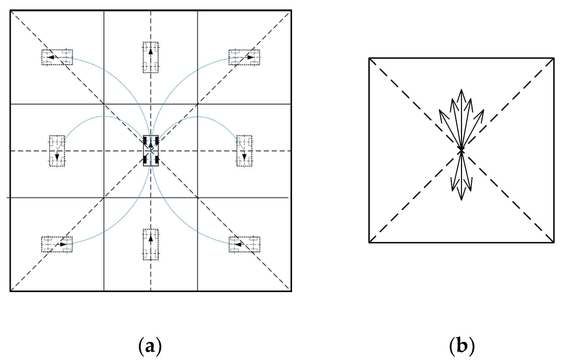
Expanding the traditional four-direction output actions to eight-direction output actions, to improve the smoothness of path planning.

(2)

Optimizing the structure of the DDQN algorithm by integrating gradient descent into the sampling process and extending it to multi-UGV systems to solve the pursuit problem.

(3)

Using the prioritized experience replay mechanism to improve the network structure and enhance speed.

The remainder of this paper is organized as follows. After reviewing the relevant literature in Section 1, the kinematic model of UGV and the environment model are given in Section 2. Section 3 presents the DDQN and prioritized experience replay. The proposed method is described in detail in Section 4. The results and discussion are provided in Section 5. Finally, conclusions and future work are presented in Section 6.

2. Materials and Methods

2.1. Problem Formulation

Multi-UGV pursuit scenarios can be described as multi-UGVs and a moving/stationary target (human or other self-propelled weaponry) to be pursued in a finite two-dimensional planar area. The task of the unmanned vehicles is to pursue the discovered target; the schematic diagram of the pursuit scenario is shown in Figure 2. In addition, in order to more closely match the actual environment of the battlefield, the following conditions are assumed in this paper.

(1)

Each vehicle obtains obstacle information through on-board LiDAR as well as cameras.

(2)

The UGVs are equipped with vehicle-to-vehicle (v2v), which can share all vehicle status and action information as well as obstacle information to ensure collaboration.

(3)

All vehicles can communicate with the ground station in real time and obtain the position and movement information of the target as obtained by the radar of the ground station.

(4)

The target can only sense the relative position of vehicles within a fixed distance $D_t$. If beyond $D_t$, the information of vehicles cannot be obtained by the target. The speed of the target is less than the maximum speed of the vehicles.

Figure 2. Initial condition of a multi-UGV pursuit scenario.

Figure 2. Initial condition of a multi-UGV pursuit scenario.

Both the UGVs and the target can move in the scene. After the vehicles obtain the location information of the target, they construct an encirclement around the target through collaboration, to realize the pursuit task. After the target senses vehicles within the distance $D_t$, it escapes from the vehicles according to a certain strategy. Let us assume that there are four vehicles performing the pursuit task, and the successful pursuit is shown in Figure 3. The vehicles are distributed around the target at equal angles to form an encircling circle to prevent the target from escaping.

2.2. Kinematic Model of UGV

The UGV‘s chassis is a four-wheeled Ackerman chassis modelled from a real experimental vehicle and consists of a heading controller (steering gear) and a speed controller (motor) that work independently. The speed control varies the torque and speed of the engine so that the UAV moves forward and backward at a predetermined speed. The heading control changes the steering angle of the front wheels so that the vehicle can follow the planned path. The kinematic model of vehicles is expressed as

$$\left[\begin{array}{c}{\dot{x}}_i\\ {\dot{y}}_i\\ {\dot{\phi }}_i\end{array}\right]=\left[\begin{array}{cc}cos{\phi }_i& 0\\ sin{\phi }_i& 0\\ 0& 1\end{array}\right]\left[\begin{array}{c}{u}_i\\ {\omega }_i\end{array}\right]$$

(1)

where $x_i,y_i,{\phi }_i$ denote the horizontal coordinate, vertical coordinate, and heading angle of the i-th vehicle, and $u_i,{\omega }_i$ denote the velocity and angular velocity. The position of vehicle $i$ at the next moment is $P_i^{\prime }=[x_i^{\prime },y_i^{\prime }]$, the heading angle is ${\phi }_i^{\prime }$, the heading angular velocity is ${\dot{\phi }}_i$, and the movement time interval is $∆t$. Then, the state of vehicle $i$ at the next moment can be described as

$$\left[\begin{array}{c}{x}_i^{\prime }\\ y_i^{\prime }\\ {\phi }_i^{\prime }\end{array}\right]=\left[\begin{array}{c}{x}_i\\ y_i\\ {\phi }_i\end{array}\right]+\left[\begin{array}{c}{\dot{x}}_i\\ {\dot{y}}_i\\ {\dot{\phi }}_i\end{array}\right]∆t$$

(2)

The UGVs need to satisfy certain motion constraints, so the state and control quantity of each vehicle need to meet

$$\left\{\begin{array}{c}{\omega }_{min}\le {\omega }_i\le {\omega }_{max}\\ a_{min}\le {\dot{u}}_i\le a_{max}\end{array}\right.$$

(3)

$$\left\{\begin{array}{c}∆{\phi }_{min}\le {\dot{\phi }}_i∆t\le ∆{\phi }_{max}\\ ∆u_{min}\le {\dot{u}}_i∆t\le ∆u_{max}\end{array}\right.$$

(4)

where ${\omega }_{min}$ is the maximum clockwise angular velocity, ${\omega }_{min}<0$; ${\omega }_{max}$ is the maximum counterclockwise angular velocity, ${\omega }_{max}>0$; $a_{min}$ is the maximum acceleration in the reverse direction, $a_{min}<0$; $a_{max}$ is the maximum acceleration in the forward direction, $a_{max}>0$. $∆{\phi }_{min}$ is the maximum angle of clockwise motion, $∆{\phi }_{min}<0$; $∆{\phi }_{max}$ is the maximum angle of counterclockwise motion, $∆{\phi }_{max}>0$. $∆u_{min}$ is the maximum velocity in the reverse direction, $∆u_{min}<0; ∆u_{max}$ is the maximum velocity in the forward direction, $∆u_{max}>0$.

In this paper, we consider multi-UGV pursuit in a 2D environment. In addition, the map needs to be rasterized. In order to simplify the computing process and combine the kinematic model, the vehicle and target can be regarded as mass points. Figure 4a shows all possible actions of the vehicle. In the grid, the vehicle can drive in eight directions, including front, back, left, right, left-front, left-back, right-front, and right-back. Since the cell edge is $l\ge 2r+w$ ($r$ is the minimum turning radius of the vehicle and $w$ is the width of the vehicle), the vehicle can normally drive to the left and right cells and stop at the center position. Figure 4b shows the heading angles corresponding to each direction of the UGV.

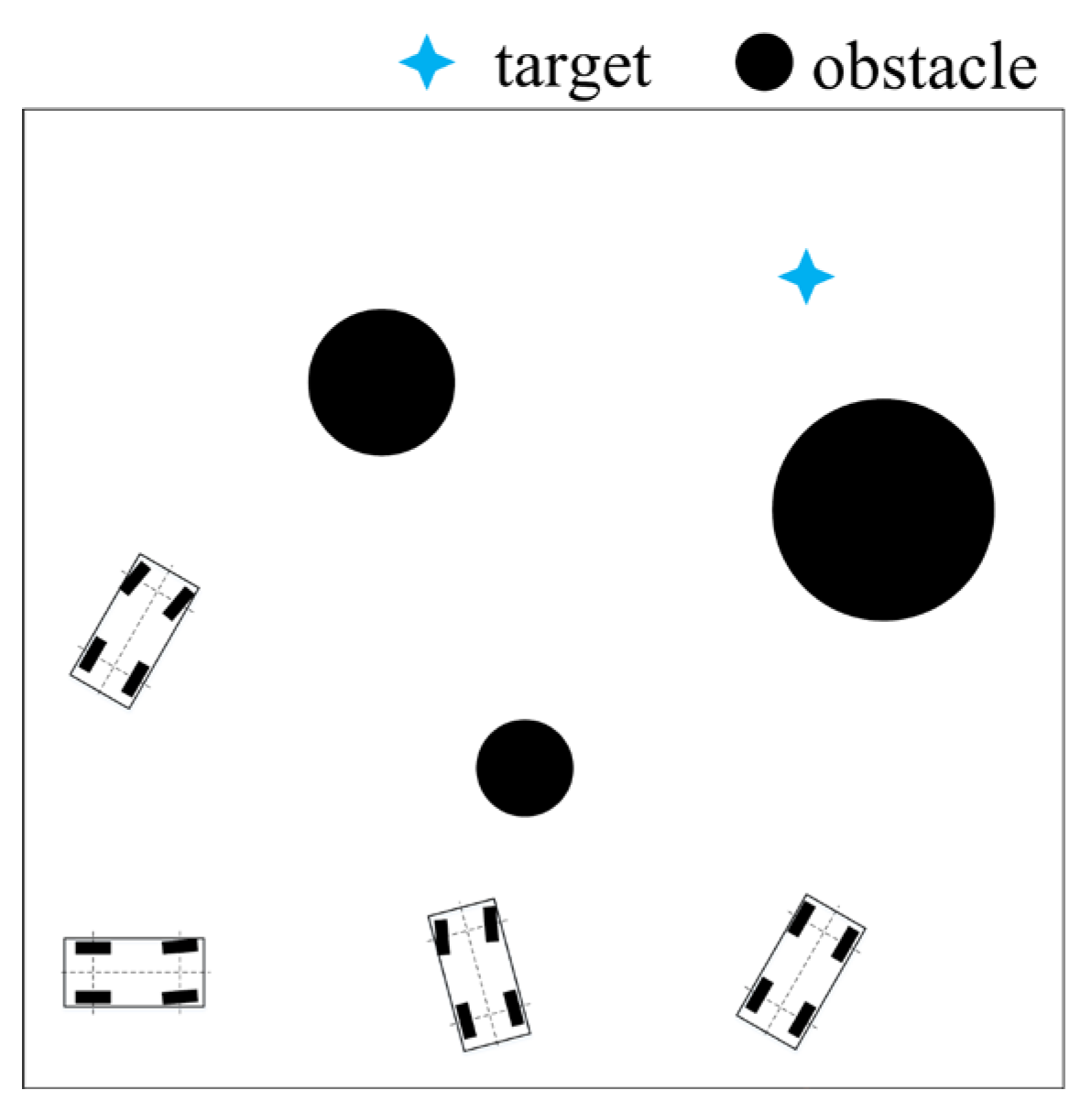
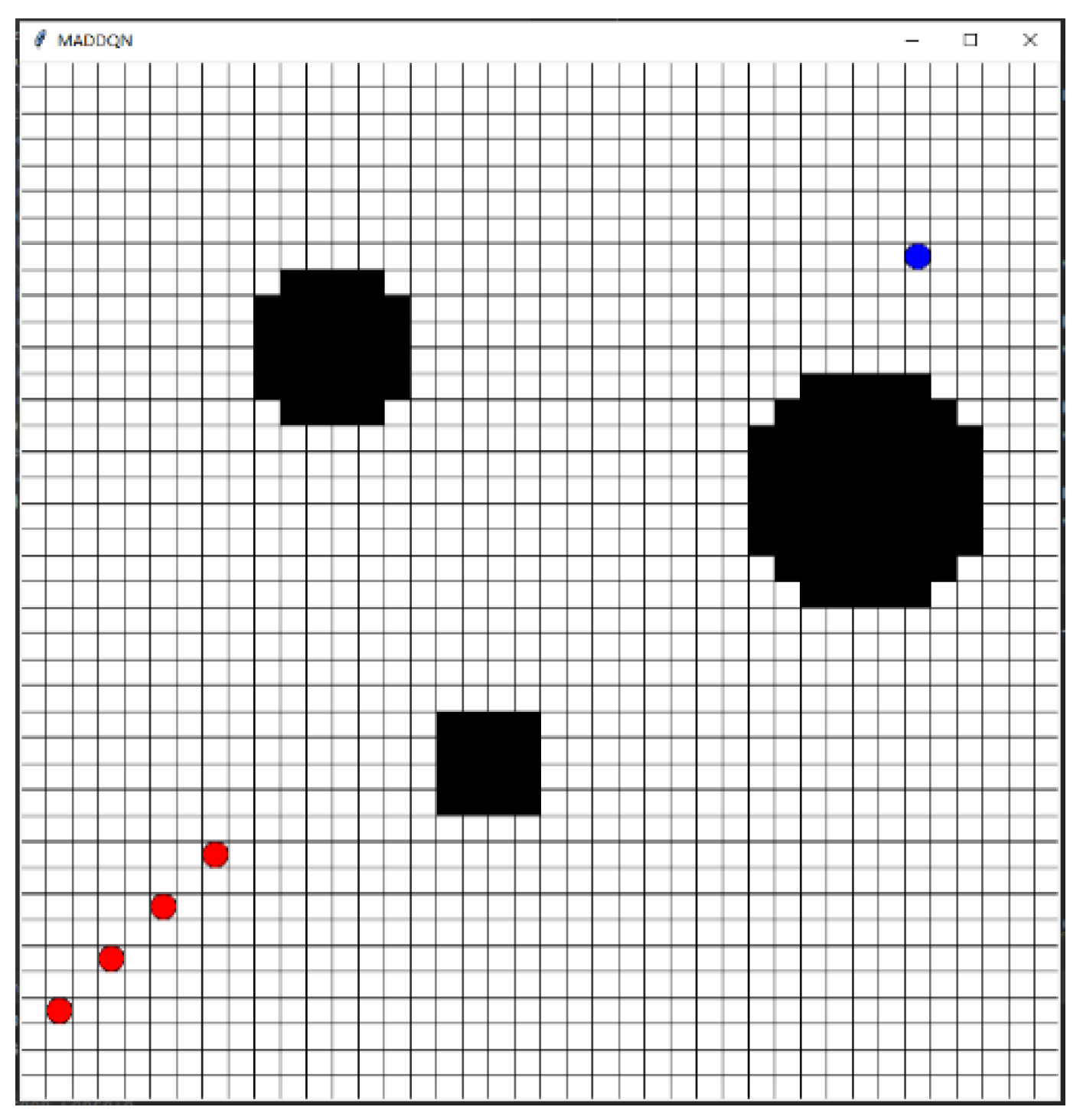
2.3. Environmental Model

Constructing the environment as a 2D map is the basis for multi-UAV pursuit path planning. It mainly aims at the unknown environment or the environment where obstacles move in real-time. For static and known environments, the subsequent planning can directly skip this process.

When constructing a 2D map, the map is divided into $M\times N$ cells, all sides of which are $l$ ($l\ge 2r+w$) in length. In order to simplify the obstacles and boundaries, the obstacles are mapped to the corresponding cells (those less than one cell are calculated as one cell), and the occupied cells are merged to facilitate the generation of passable paths by the proposed algorithm. Figure 5 shows the map construction process used to create the distance matrix and reward matrix. Figure 5a is the 2D map. Cells of side length $l$ are divided on the boundary and obstacles, corresponding to the cell map in Figure 5b.

The simulation employs the Tkinter toolkit for constructing the environment model and utilizes the Pytorch learning library for training purposes. For the experiment, an environment model diagram with a cell size of 40 × 40 and a resolution of 20 pixels per cell is constructed. The vehicles operate and make decisions within this environment model. The number of cells in the environment corresponds to the number of states through which the vehicles navigate, as depicted in Figure 6. In total, there are 1600 states. The vehicles are visually represented by red circles in Figure 6, while the target is represented by a blue circle. These circles are enclosed within a rectangle, and with each action executed, the circles move one cell on the map. In Tkinter, the representation of rectangular coordinates is based on the intersection coordinates of two diagonal lines, which eases the convenience of position representation. The initial positions of the vehicles are set as (1, 36), (3, 34), (5, 32), and (7, 30), with the target set at (34, 7). Passable areas are depicted as cells, while the obstructed areas are depicted as black cells in Figure 6. By adjusting the coordinates, the program allows for changes in the positions of the vehicles and the target on the map. The environment interface enables the retrieval of the real-time positions of the vehicles, which provides a visual depiction of the shortest path taken, to assist with the setup and adjustment of the neural network parameters.

3. Deep Reinforcement Learning

DRL mainly obtains experience through interaction with the external environment and evaluation feedback and makes behavioral decisions according to system performance [31]. DRL can improve the performance of the system through repeated trials in dynamic environments and provide qualitative or quantitative feedback via rewards and penalties to understand the task and achieve the set goal. The planning algorithm based on DRL integrates all the equipment and software in the multi-UGV system to identify the optimal behavior to be taken by referring to the maximization of the reward output action in the given situation. Based on the DDQN algorithm, the proposed method interacts with the environment through perception and action and takes the perceived environmental information as input and the corresponding action generated by planning as output. Then, the optimal trajectory sequence is formed to complete the pursuit task.

3.1. Q Functions

Q learning is a type of DRL algorithm based on Markov theory. The reward, action, and strategy are considered simultaneously in the Markov chain; that is, the state transition is executed by the action to form the Markov decision process. In order to better understand the Markov decision process, this paper introduces the concept of return. The return $G_t$ is the sum of the reward discounts of each step in the steps, expressed as

$$G_t=r_t+\gamma r_{t+1}+{\gamma }^2{r}_{t+2}+{\gamma }^3{r}_{t+3}+\cdots$$

(5)

The discount factor $\gamma$ is an important mathematical parameter used to reintegrate the return value. The value of $\gamma$ is always set between 0 and 1: when $\gamma =0$, $G_t$ considers only immediate rewards; when $\gamma =1$, future rewards have the same status as immediate rewards and have the same effect on returns.

The update of the state-value function is presented as

$$V\left(s\right)=E\left[G_t|s_t=s\right]=E[r_t+\gamma r_{t+1}+{\gamma }^2{r}_{t+2}+{\gamma }^3{r}_{t+3}+\cdots |s_t=s]$$

(6)

By rearranging the items in (6), the state-value function is equal to the sum of the discount factor, the probability caused by the previous state and the product of the three terms of the next state-value function, plus the immediate reward $R\left(s\right)$ of the state, which can be written as

$$V\left(s\right)=R\left(s\right)+\gamma {\sum }_{s^{\prime }\in s}P\left(s^{\prime }|s\right)V\left(s^{\prime }\right)$$

(7)

The action influence is added to the state-value function and the policy function is established:

$$\pi \left(S\right)={\sum }_{a\in A}\pi \left(a|S\right)R\left(S,a\right)$$

(8)

$$P^{\pi }\left(S^{\prime }|S\right)={\sum }_{a\in A}\pi \left(a|S\right)P\left(S^{\prime },a\right)$$

(9)

After considering strategy $\pi$, the state-value function in (7) can be rewritten as

$$V_k^{\pi }\left(s\right)=r\left(s,\pi \left(s\right)\right)+\gamma {\sum }_{s^{\prime }\in s}p\left(s^{\prime }|s,\pi \left(s\right)\right)V_{k-1}^{\pi }\left(s^{\prime }\right)$$

(10)

The optimal $q$ function can be written as

$$q^{\mathrm{*}}\left(s,a\right)=\mathit{max}q\left(s,a\right)$$

(11)

According to the $q$ function in (11), the strategy should choose the highest $q$ value to obtain the future overall reward. In order to obtain the optimal value$,$ the Bellman equation must be satisfied. Therefore, (11) can be rewritten as

$$q^{\mathrm{*}}\left(s,a\right)=E\left[R_{t+1}+\gamma max{q}^{\mathrm{*}}\left(s^{\prime },a^{\prime }\right)\right]$$

(12)

(12) represents the optimal $q$ value of a given state–action $(s,a)$ which is equal to the expected reward $R_{t+1}$ after taking the action plus the expectation of discount reward for the $\left(s^{\prime },a^{\prime }\right)$ optimal policy. If the state space is relatively simple, a linear function approximator can be used to find the $q^{\mathrm{*}}$ value. However, in a complex environment, the performance of the linear function approximator is far from sufficient. Generally, nonlinear function approximators (such as neural networks) can be used to approximate the optimal $q^{\mathrm{*}}$ value.

3.2. Value Function Update

The multi-UGV system performs the task autonomously according to the training dataset. Without sufficient training datasets, the vehicles can only learn from experience. Since the system is limited to a specific mapping model, each vehicle must explore the same environment several times in order to achieve optimal planning. Therefore, autonomous vehicles operating in the environment must balance the utilization of old datasets with the exploration of new data, so that each autonomous vehicle can learn to find a better path. The utilization of old datasets means that each unmanned vehicle makes use of the existing global environment and results and plans the path of each vehicle based on the existing datasets. New data exploration aims to discover new conditions and features of the environment and find a better path than the previously known optimal path. Using the two updating methods, the multi-UGV system is able to perform optimal path planning, even in an unknown environment [32].

The idea of Q-learning is to find the best action sequence, and the goal is to maximize the return value ($G_t$) defined in (5). Combining (10) and (11), deterministic methods and probabilistic rules can be used to complete the update. For deterministic scenarios, action $a$ needs to be performed, reward $r$ is obtained in state $s$, and the value of $Q\left(s,a\right)$ is updated by adding $Q\left(s,a\right)$ to the previous value. Thus, $Q\left(s,a\right)$ can be written as

$$Q\left(s_t,a_t\right)\leftarrow r+\gamma \underset{a_{t+1}}{\mathit{max}}Q\left(s_{t+1},a_{t+1}\right)$$

(13)

The learning rate $\alpha$ is introduced, and the probability update rule can be calculated as

$$Q\left(s_t,a_t\right)\leftarrow \left(1-\alpha \right)Q\left(s_t,a_t\right)+\alpha \left[r+\gamma maxQ\left(s_{t+1},a_{t+1}\right)\right]$$

(14)

$Q\left(s,a\right)$ is updated in the neural network, and the learning rate $\alpha$ is utilized to control the update rate and impact $Q\left(s,a\right)$. Initially, a large learning rate $\alpha$ is employed to facilitate updates during the early stages of training. Over time, the learning rate $\alpha$ gradually decreases to minimize its influence on the update of $Q\left(s,a\right)$. Specifically, an initial value of 0.03 is assigned to $\alpha$, which subsequently decreases by a rate of 0.0002 per episode until reaching 0.001. The rationale behind this design choice is grounded in the fact that $Q\left(s,a\right)$ in the neural network may occasionally contain noise or incorrect values. Whenever the observed state–action value is determined to be optimal at a given time, it is necessary to update $Q\left(s,a\right)$. However, as training progresses and $Q\left(s,a\right)$ values in the experience replay become more accurate, extensive changes to the accurate $Q\left(s,a\right)$ may lead to a deterioration in training effectiveness. Consequently, the introduction of a gradually decreasing factor $\alpha$ helps to modulate the impact of $Q\left(s,a\right)$ updates over time and ensures stable training progress.

In order to understand Q-learning more accurately, three parameters are very important: one is the maximum number of episodes in the learning process; the second is the random exploration value, which determines whether the algorithm can avoid entering an infinite loop between actions during learning; and the third is the temporal difference (TD) [33], which is used to evaluate the learning process and can be directly calculated from the Q-learning expression in (14). The value of TD can be obtained by rewriting and removing the learning rate component

$$TD\left(t\right)\leftarrow r+\gamma \underset{a_{t+1}}{\mathit{max}}Q\left(s_{t+1},a_{t+1}\right)-Q\left(s_t,a_t\right)$$

(15)

The sum of TD in each episode is the cumulative error expressed as

$$T{D}_{acc}={\sum }_{t=0}^{t_{max}}TD\left(t\right)$$

(16)

3.3. Double Deep Q-Learning

This paper focuses on DDQN [34]. This is because although DQN [35] is suitable for planning tasks, it suffers from the issue of q-value overestimation. To address this problem, DDQN employs two separate networks: the estimated network and the target network. By separating the action-selection process from the generation of target q-values, DDQN significantly reduces the q-value overestimation to not only facilitate faster training but also enhance the stability of learning. The DDQN algorithm separates selection and interpretation and simultaneously takes two Q functions as the target. The Q function is shown as

$$Q\left(s_t,a_t\right)=r_t+Q\left(s_t,a_t\right)=r_t+\gamma Q\left(s_{t+1},\underset{a_{t+1}}{\mathit{argmax}}Q\left(s_{t+1},a_{t+1};\theta \right);{\theta }^{-}\right)$$

(17)

3.4. Prioritized Experience Replay

DDQN utilizes random samples from an experience replay for training. In the original DDQN, all samples are selected with the same probability. However, Dang et al. [36] introduced the prioritized experience replay mechanism to address this limitation. This mechanism assigns different weights to different samples, thereby altering the probability of selecting samples during training. The weights are determined based on the performance of the samples, giving higher weights to samples that exhibit good training results.

To implement this mechanism, a queue structure is used to store experiences at the beginning of training. When the experience replay is full, newly generated samples are compared with the existing samples in terms of weight. If the latest sample has the minimum weight, it is discarded. On the other hand, the latest sample replaces the sample with the minimum weight in the experience reply memory. By dynamically updating the weights of the samples, prioritized experience replay ensures that samples with higher weights have a greater probability of being selected during the training process. This approach shifts the focus to determining the sample weights rather than treating all samples equally.

In the DDQN algorithm, TD is the difference between the current q-value and the target q-value, which represents the magnitude of the correction and can be used as an important index to measure the sample weight. The specific formula for calculating TD is shown in (15). The higher the value, the lower the number of samples. This means that the corresponding sample occurs less and the accuracy of the sample needs to be improved. Improving the priority of such samples to improve the utilization of these samples will increase the DDQN learning speed significantly.

The sampling probability of a sample is defined as

$$p\left(j\right)=\frac{P_j^{\alpha }}{\sum _i{P}_i^{\alpha }},\alpha \in [\mathrm{0,1}]$$

(18)

where $P_j$ is the priority indicator, i.e., $TD\left(t\right)$ in (15); α is the priority adjustment parameter that ensures that all experiences have at least one chance of being drawn.

With the introduction of the prioritized experience replay, the DDQN favors samples with higher TDs, which changes the probability distribution of the original samples but generates errors that prevent the convergence of training. Therefore, it is necessary to use importance sampling to update the sample weights during calculation of the weight change, to correct the error; this is expressed as follows:

$$W_j={\left(\frac{1}{MP\left(j\right)}\right)}^{\beta }$$

(19)

where $M$ is the memory size and exponent $\beta$ is the level of correction.

4. Multi-UGV Pursuit Algorithm

In order to complete the task of multi-UGV pursuit, the path-planning algorithm needs to read the map of the environment. Then, the optimal path to capture the target is planned on the premise of avoiding obstacles and other vehicles. A DDQN-based algorithm is proposed in this paper for multi-UGV pursuit by integrating the prioritized experience replay and gradient descent to optimize the algorithmic framework, to accomplish the pursuit task with faster speeds and smoother paths.

4.1. State Representation

The state information of UGVs mainly includes three components:

(1)

The state information of the vehicle itself, including the position information, heading angle, speed, and detection information of the vehicle to obstacles; this can be expressed as

$$S_i^{self}=[x_i,y_i,{\phi }_i,u_i,x_i^{o0},y_i^{o0},\dots ,x_i^{o(k-1)},y_i^{o(k-1)}]$$

(20)

where $k$ is the number of obstacles, and $x_i^{o(k-1) }\mathrm{a}\mathrm{n}\mathrm{d} y_i^{o(k-1)}$ are the relative distances of the obstacle $k-1$ to vehicle $i$ in the x and y directions, respectively.

(2)

The target information, including the real-time velocity information and relative position information of the target from the ground station; this is expressed as

$$S_i^{tar}=[u^{tar},x_i^{tar},y_i^{tar}]$$

(21)

(3)

The teammate information, including the speed information of other vehicles and the relative distance information; this can be described as

$$S_i^{oth}=[u_i^0,x_i^0,y_i^0,\dots ,u_i^{i-1},x_i^{i-1},y_i^{i-1},u_i^{i+1},x_i^{i+1},y_i^{i+1},\dots u_i^{n-1},x_i^{n-1},y_i^{n-1}]$$

(22)

where $n$ is the number of vehicles.

In summary, the state representation of vehicle $i$ is

$$S_i=[S_i^{self},S_i^{tar},S_i^{oth}]$$

(23)

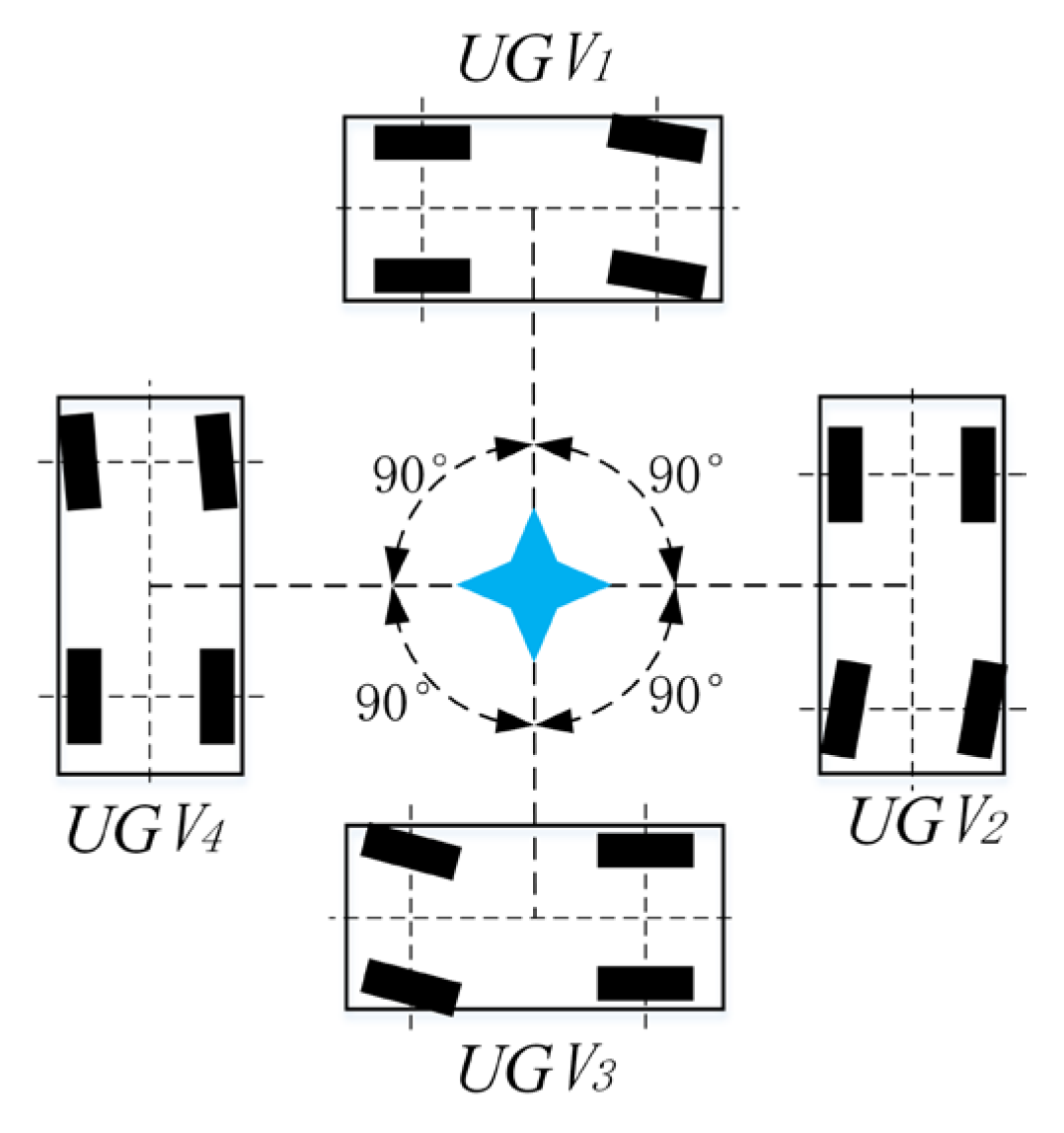
4.2. Action Space

The action space is defined as the motion process in each direction in the state space, i.e., each action represents a different direction of the motion performed, as shown in Figure 4. The acceleration control and direction control of the vehicle are divided into eight cases according to the action space, as shown in

Table 2. Parameters for the action space.

Direction	$\mathbf{Acceleration} (\mathbf{m}/{\mathbf{s}}^2)$	$\mathbf{Angular} \mathbf{Velocity} (\mathbf{r}\mathbf{a}\mathbf{d}/\mathbf{s})$
Front	1.0	0
Left-front	0.5	0.5
Left	0	1.0
Left-back	−0.5	0.5
Back	−1.0	0
Right-back	−0.5	−0.5
Right	0	−1.0
Right-front	0.5	−0.5

. The action space consists of a 1 × 2 array, denoted as $A_i=\{a_i,{\omega }_i\}$, with $a_i$ denoting the acceleration and ${\omega }_i$ denoting the angular velocity of the i-th vehicle.

4.3. Reward Function

(1)

Reward matrix design

The reward matrix is obtained from the distance matrix. The distance matrix is shown in Figure 7a. The value in the matrix is the distance between the cell and the end cell. The red cell is the end point and the values in the cells in Figure 7a are the distances of the cells to the end point. Figure 7b shows the reward matrix, where the values (in minus −) in the matrix represent the reward from any place on the map to the end point.

In addition, it is also necessary to consider the environment boundaries and the obstacles in the environment. In these cases, the reward is actually a penalty to the algorithm and it is clear that the vehicles should not move to the cell containing obstacles and boundaries. Generally, the cells containing obstacles and boundaries are assigned a value much lower than the reward (for example, −1000) in the reward matrix.

Once the reward matrix is generated, the neural network used in the learning process can be constructed. The neural network contains the actions and states of all vehicles at each moment.

(2)

Reward mechanism design

The maximum number of training steps in a single episode is 3500, and the training can be terminated if any of the following conditions are met:

①

The vehicle reaches a distance of 1 to the target and does not collide with boundaries and obstacles.

②

The algorithm reaches 3500 steps and does not collide with the boundary and obstacles, but also does not reach the vicinity of the target.

③

The vehicle collides with the boundary or obstacle, or collides with other vehicles during travel.

According to the above conditions, the vehicle reward mechanism is designed as in

Table 3. Reward mechanism for training.

Action	Reward	Result
Vehicle collides with other vehicles/boundaries/obstacles	−1000 value in the reward matrix	Terminated
Vehicle in passable areas	Value in the reward matrix	Continue
Vehicle arrives at a distance of 1 from the target	1000	Terminated

.

4.4. Gradient-Descent-Based Path Smoothing

Path smoothing is very important in path planning; it aims to make the path length shorter and the smoothness higher, so as to adapt to the passage of the unmanned vehicles.

Huang et al. [37] used the K-degree smoothing method to smooth the initial path; this could make the UAVs reach the destination within an acceptable time interval; however, the environment model was relatively simple and not suitable for a dynamic environment. To obtain a smooth path that satisfies constraints such as obstacle avoidance, minimized cost, and dynamic feasibility, Dian et al. [38] constructed an optimization problem for smooth path planning based on the length and the requirement of collision-free safety. By utilizing a high-order continuous Bezier curve, the smooth-path-planning problem is transformed into an optimization problem that searches the locations of control nodes of the Bezier curve. This methodology enables the generation of a path that satisfies the specified constraints. Song et al. [39] used the continuous high-order Bezier curve to replace continuous multiple low-order Bessel curve segments. However, the adjustment of weight coefficients in the continuous high-order curve mainly depended on experience, which makes it struggle to achieve optimal convergence.

In this paper, the path generated by the gradient descent algorithm is smoothed. The goal of the gradient descent is to improve the quality of the given feasible path $\sigma$ generated by the motion planner. The algorithm is divided into a split and merge, which approximates the curve linearly by subdividing line segments at the higher error vertices and merging adjacent segments whilst maintaining the error range.

Given a path $\sigma$ and transition function $T_r,$ the smoothing is mainly divided into two stages; in the first stage, the path is deformed by moving and inserting the vertices to increase the distance from the obstacle and sample enough vertices in the area close to the obstacle; in the second stage, the vertices are removed from the path using cost-aware path short-cutting, as shown in Figure 8.

(1)

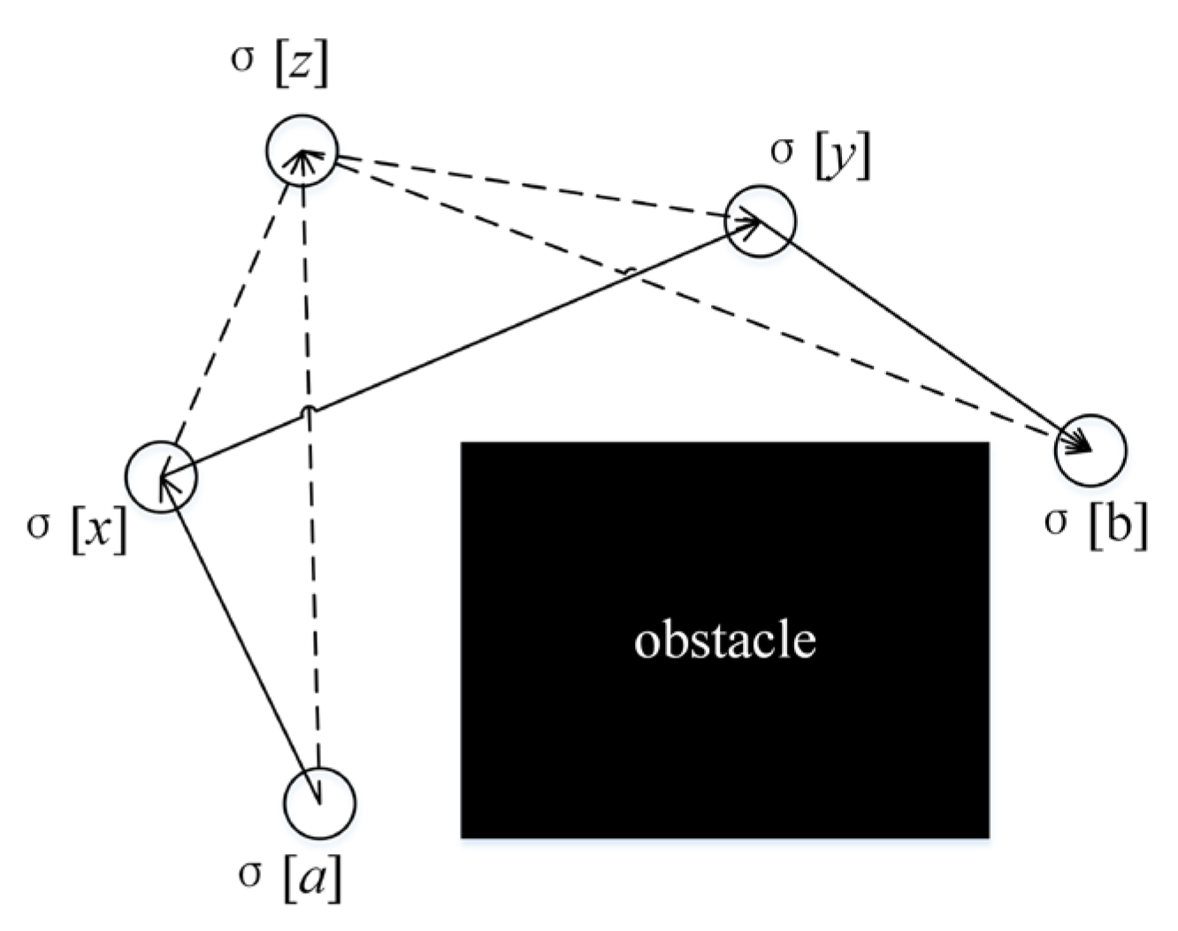
Gradient-based path deformation: this algorithm moves and inserts the vertices in the obstacle distance field D through gradient descent, where the obstacle distance is calculated as

$$D\left[p\right]=\underset{o\in \mathcal{O}}{\mathit{min}}{‖o-p‖}_2$$

(24)

where $p$ is the continuous vertex position and $O$ is the coordinates set occupying the cell. As long as the distance matrix to the obstacle cells has been precomputed, $D\left[p\right]$ can be determined in constant time by linear interpolation between the cells adjacent to $p$.

The gradient $𝛻D$ in the distance field is

$$𝛻D\left[p\right]=\left(\begin{array}{c}\frac{D\left[p.x-ϵ,p.y\right]-D\left[p.x+ϵ,p.y\right]}{2ϵ}\\ \frac{D\left[p.x,p.y-ϵ\right]-D\left[p.x,p.y+ϵ\right]}{2ϵ}\end{array}\right)$$

(25)

where $ϵ$ is a small constant and $ϵ>0$.

Gradient descent moves the vertex $p$ by $-\eta 𝛻D\left[p\right]/D\left[p\right]$, where $\eta$ is the step size (${\eta }_0$ is the initial value) multiplied by the discounting factor $\mu \in \left(0,1\right]$ in each gradient descent round; furthermore, $-\eta 𝛻D\left[p\right]$ defines the direction in the distance field.

Figure 8. Diagram of gradient descent algorithm.

Figure 8. Diagram of gradient descent algorithm.

(2)

Cost-aware path short-cutting: Short-cutting is used to remove the vertices of unnecessary turns to prevent high arc length and large curvature. Firstly, it identifies a vertex that cannot be passed directly (i.e., the path jumps directly from the previous to the next point). A directed acyclic graph is then constructed for each pair of consecutive immovable vertices $\sigma \left[a\right]$ and $\sigma \left[b\right]$; its vertex $\sigma [a:b]$ is the vertex of the path segment and its edge is the collision-free steering connection between these vertices. It finds the best path from vertex $\sigma \left[a\right]$ to vertex $\sigma \left[b\right]$ and removes all vertices $\sigma [a:b]$ in the path segment ${\sigma }_{ab}^{\mathrm{*}}$ that are not on the path. The cost-aware path short-cutting iterates over the entire path until no more vertices can be removed or the maximum number of rounds has been reached.

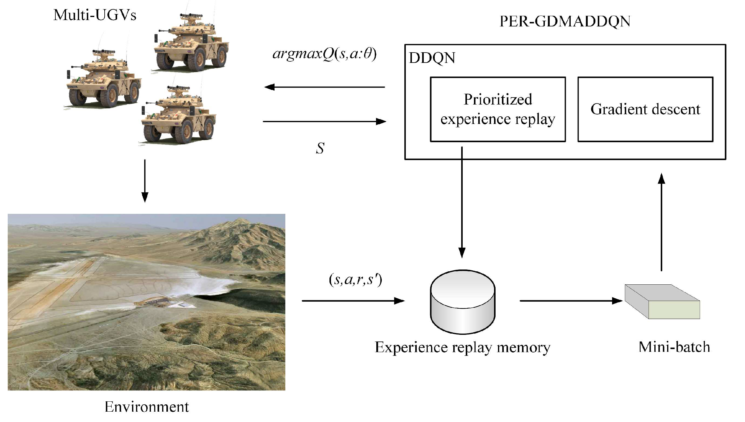
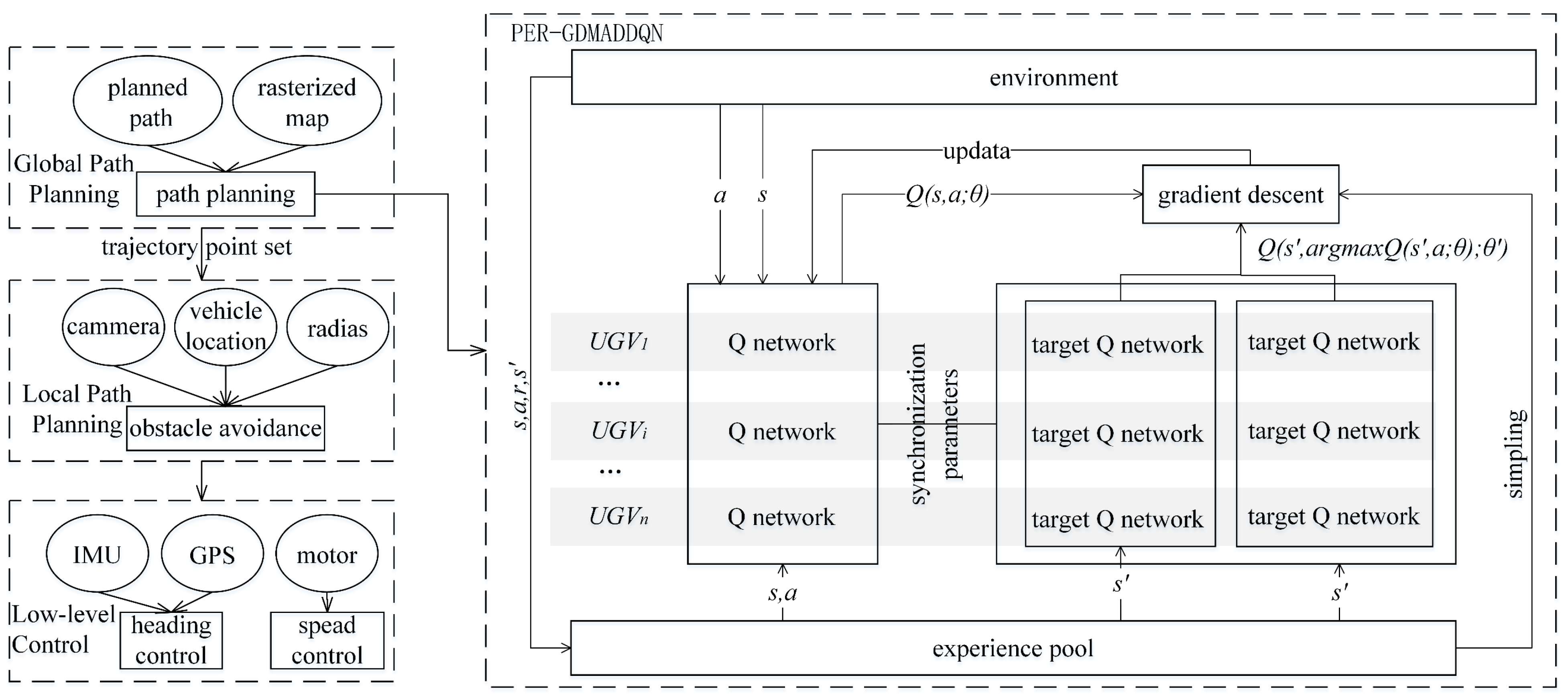
4.5. Pursuit Algorithm Flow

The planning architecture organization of multi-UGVs is shown in Figure 9. The low-layer is based on the bicycle motion model, and the upper-layer is mainly based on local and global path-planning modules. The function of local path planning is to plan local alternative paths according to the obstacle information in the map, to avoid obstacles. The top layer performs global path planning, which mainly plans the optimal path according to the map information and the information of all unmanned vehicles. A PER-GDMADDQN algorithm is proposed to plan the global optimal path of all unmanned vehicles.

The basic processing flow of the proposed PER-GDMADDQN algorithm in this paper is described as

①

create a rasterized map of the terrain to obtain a discrete description of the environment,

②

view the obstacle location and size and learn safe paths based on the proposed algorithm, and

③

train the algorithm to find safe and feasible paths that can be passed to the local path-planning layer.

The algorithm begins by interacting with the environment to obtain new states and actions. The gradient descent method is then introduced into the planning results for smoothing, and these results are packed into samples that are stored in the experience replay. In the training process, the algorithm updates the target network parameters based on the prioritized experience replay mechanism. This is performed via probabilistically sampling from the experience replay according to the weights assigned to each sample. The target network parameters are updated first, and then the two updated target networks are combined to update the estimation value network. The TD is recalculated based on the updated network and updated in the corresponding samples within the experience replay.

The algorithm begins by interacting with the environment to obtain new states and actions. The gradient descent method is then introduced into the planning results for smoothing, and these results are packed into samples that are stored in the experience replay. In the training process, the algorithm updates the target network parameters based on the prioritized experience replay mechanism. This is performed by probabilistically sampling from the experience replay according to the weights assigned to each sample. The target network parameters are updated first, and then the two updated target networks are combined to update the estimation value network. The TD is recalculated based on the updated network and updated in the corresponding samples within the experience replay. The practical flows is shown in Algorithm 1.

Algorithm 1 Multi-UGV pursuit algorithm

1 Initialize the 2D environment, exploration probability $ϵ$, discount factor $\gamma$, q value updating factor $\alpha$; 2 for episode = 0 to M-1 do 3     Initial position joint state information $s_0=\left(S_{10},\dots ,S_{n0}\right)$, $S_{i0}=(x_{i0},y_{i0})$, $S_{i0}$ is obtained from the information shared through the communication; 4     while episode not terminated do 5         for vehicle $i=0$ to $n-1$ do 6             take random $\rho \in \left(\mathrm{0,1}\right)$; 7             if $ϵ>\rho$ then 8                 Take random action $a_{it}$ from action space; 9             else 10                 action $a_{it}=\mathrm{a}\mathrm{r}\mathrm{g}\mathrm{m}\mathrm{a}{\mathrm{x}}_{a}Q\left(s_t,a\right),s_t\in (S_{1t},\dots ,S_{nt})$; 11              Decay exploration probability $ϵ\left(i\right)$; 12              Execute action $a_{it}$, then observe reward $r_{it}$ and next state $s_{t+1}$; 13              Experience value $e_t=(s_t,a_{it},r_{it},s_{t+1})$ is stored into experience replay memory E according to priority $P_t=\mathrm{m}\mathrm{a}\mathrm{x}{P}_i.$ The stored path is smoothed based on gradient descent; 14              for $j=1$ do 15                  Sampling according to $P_j$: $j~P\left(j\right)=\frac{P_j^{\alpha }}{\sum _i{P}_i^{\alpha }}$; 16                  Calculate the importance sampling weights according to Equation (19); 17                  Calculate $TD\left(t\right)$ according to Equation (15); 18                  Update the sample priority: $P\left(j\right)\leftarrow TD\left(t\right)$; 19              if episode terminates at $s_{k+1}$ then 20                  if collision or all pursuit successful then 21                      $y_k=\sum _1^n{y}_{ik}=\sum _1^n{r}_{ik}$; 22                      obtain the state $(s_{i0,}{s}_{i1},\cdots ,s_{it})$ of each vehicle from E, and plan the path curve; 23                  else 24                      $y_{ik}=r_{ik}$; 25              else 26                  $y_{ik}=r_{ik}+\gamma \underset{a}{\max }Q\left(s_{t+1}\right(i\left)\right)$; 27                  Compute the loss function $loss={\sum _1^n\left(y_{ik}-Q\left(s_k,a_{ik}\right)\right)}^2$; 28                  Execute the optimization algorithm on the loss function to update the Q-network for back propagation; 29                  $s_t{=s}_{t+1}$;

During the testing phase, each unmanned vehicle employs its respective neural network to calculate a sequence of actions that maximizes the reward value given a particular state. These actions are then mapped onto the environment to derive the planning path, which represents the optimal path.

5. Experiment Evaluation and Results

In the experimental evaluation, the proposed method was compared with some popular algorithms such as MADDPG [20], Regularized Softmax Deep Multi-Agent Q-Learning Network (RES-MADQN) [40], and A* for a pursuit task.

5.1. Parameter Setting

The simulation environment was an Ubuntu 18.04 and Anaconda3 platform, the experimental program was based on Python 3.6. A 2D environment was built using the Python standard library Tkinter, and the neural network was built based on Pytorch. The sampling time interval between two adjacent times was set to 1 ms. All results were obtained on the Intel Core i7-11800H CPU and NVIDIA GeForce RTX 3060 GPU.

After several tests, the parameter settings of the proposed algorithm in this paper were obtained as shown in

Table 4. Hyper-parameters list.

Hyperparameters	Value	Description
$\gamma$	0.90
Initial $\epsilon$	0.90	Explore the initial value $\epsilon$
Final $\epsilon$	0.1	Explore the final value $\epsilon$
Minibatch	32	Size of the sample
Learning rate	0.03	Learning rate of the optimizer
Experience replay	10,000	Capacity of experience replay
Memory	True	—
Network type	CNN	—
Activation function	ReLU	Learning complex patterns in data

. The parameter settings of the MADDPG and the RES-MADQN are the same as those of the proposed algorithm.

5.2. Static Targets Pursuit

There are four UGVs to pursue one static target in the simulation. The performance of the proposed PER-GDMADDQN is compared with that of the MADDPG and RES-MADQN algorithms. In the comparison, the initial conditions for different algorithms are the same. The optimal path, number of iteration steps per episode, time consumption, and reward of each algorithm are shown in Figure 10, Figure 11, Figure 12, and Figure 13, respectively.

The simulation results from the starting position to the target position using the MADDPG in the grid environment are shown in Figure 10a and Figure 11a. The shortest total path is 185 steps and the longest path is 3828 steps. The RES-MADQN results are shown in Figure 10b and Figure 11b. The shortest path is 129 steps and the longest path is 3506 steps. The results of the proposed algorithm are shown in Figure 10c and Figure 11c. The shortest path is 120 steps and the longest path is 3071 steps. As can be seen, the path-planning performance of the proposed method is better than MADDPG and RES-MADQN.

In the training process, since there is no signal accumulation at the early stage of learning, it takes a lot of time to find the path at the beginning, and obstacles are constantly encountered in this process. However, as the knowledge accumulates, the number of steps required for the wayfinding process gradually decreases. Figure 12a shows that the MADDPG algorithm has no obvious convergence trend in the process of 10,000 episodes. Figure 12b shows that the RES-MADQN algorithm tends to converge at around 6000 episodes through continuous exploration of the environment and accumulation of knowledge. Figure 12c shows that the convergence speed of the proposed PER-GDMADDQN algorithm is significantly faster and converges at around 4000 episodes, which is nearly 2000 episodes less than the convergence speed of the RES-MADQN. In the same environment, the MADDPG algorithm requires 48,525 ms for training, the RES-MADQN algorithm requires 408 ms, and the proposed algorithm requires 311 ms.

The DRL accumulates rewards in the learning process and maximizes the cumulative reward value as the learning objective. At the start of learning, the vehicle actions are randomly selected, and it is easy to encounter obstacles. When an obstacle is encountered, the reward value is −1000, so the initial reward value is negative. With the increase in training episodes, the number of vehicles encountering obstacles decreases, and the cumulative reward increases gradually. It can be seen in Figure 13a that when the training number increases, the cumulative reward of the MADDPG algorithm does not converge. As can be seen in Figure 13b, the cumulative reward of the RES-MADQN algorithm gradually increases with the increase of training episodes and finally approaches −3500. Figure 13c shows that the cumulative reward variation of the proposed algorithm is more stable and approaches −2600 at about 4000 steps. The three trained models are applied to the same obstacle environment, and three planned paths are obtained. The path information is listed in

Table 5. Comparison of the algorithms for path planning.

	MADDPG	RES-MADQN	PER-GDMADDQN
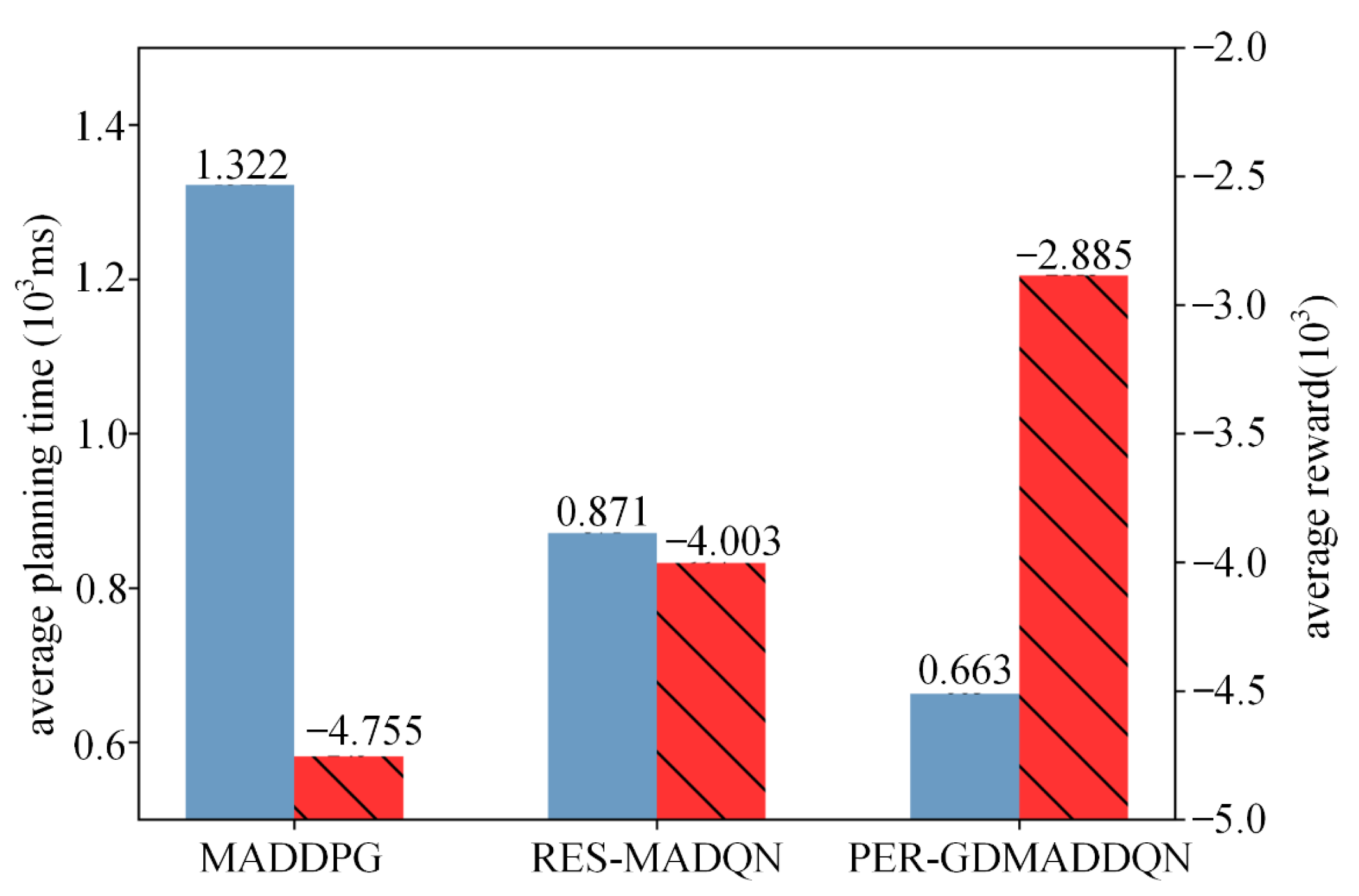
Planning time (ms)	882	561	419
Number of turns	18	10	6

.

As can be seen in the table, PER-GDMADDQN is much better than MADDPG and RES-MADQN in terms of planning time. This is mainly because the proposed algorithm introduces the prioritized experience replay, which substantially reduces the training time and makes it easier to obtain the optimal path. In addition, the total path after smoothing is compared to the unsmoothed path, and the planning time is reduced by a certain magnitude. The smoothing can be shown in the number of turns, and it can be seen from Table 5 that the proposed algorithm has a significantly lower number of turns than the other two algorithms due to the use of gradient descent.

The simulation results are listed in

Table 6. Performance comparison of the three algorithms.

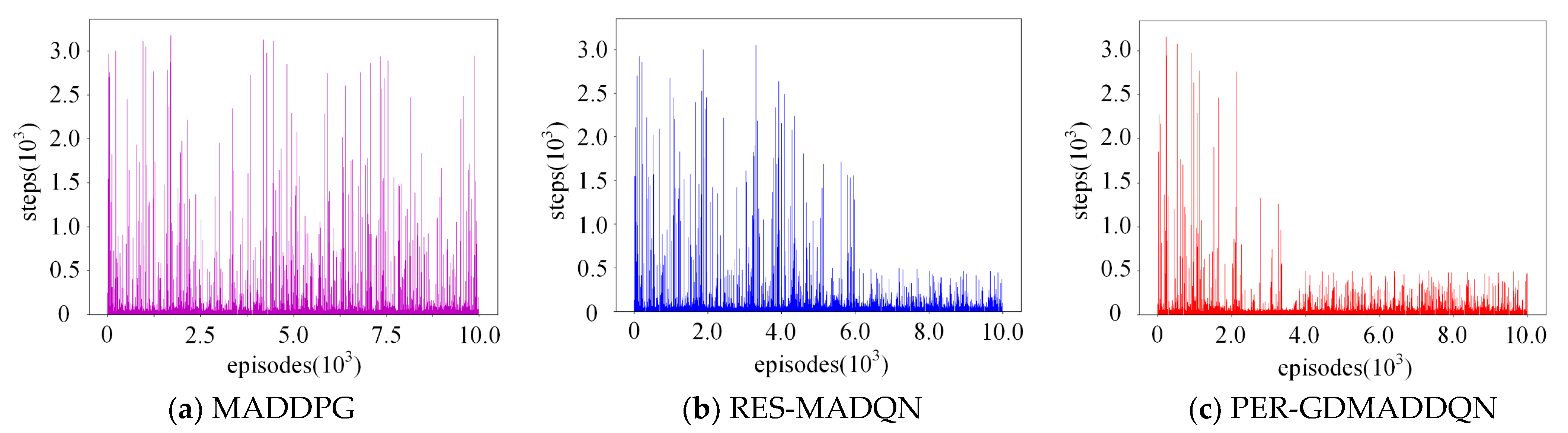
Performance	MADDPG	RES-MADQN	PER-GDMADDQN
Minimum steps	185	129	120
Maximum steps	3828	3506	3071
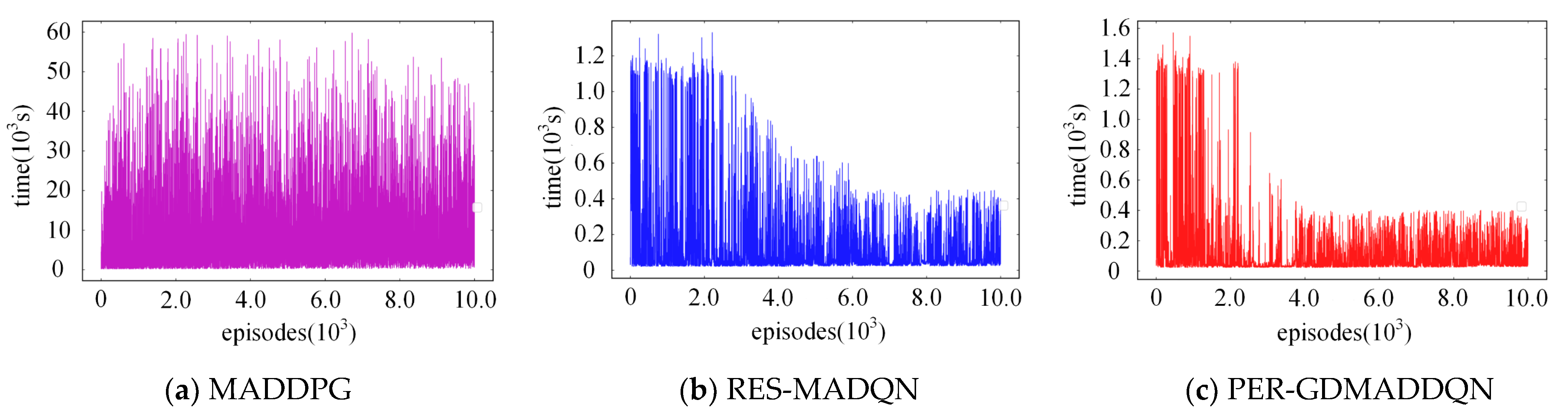
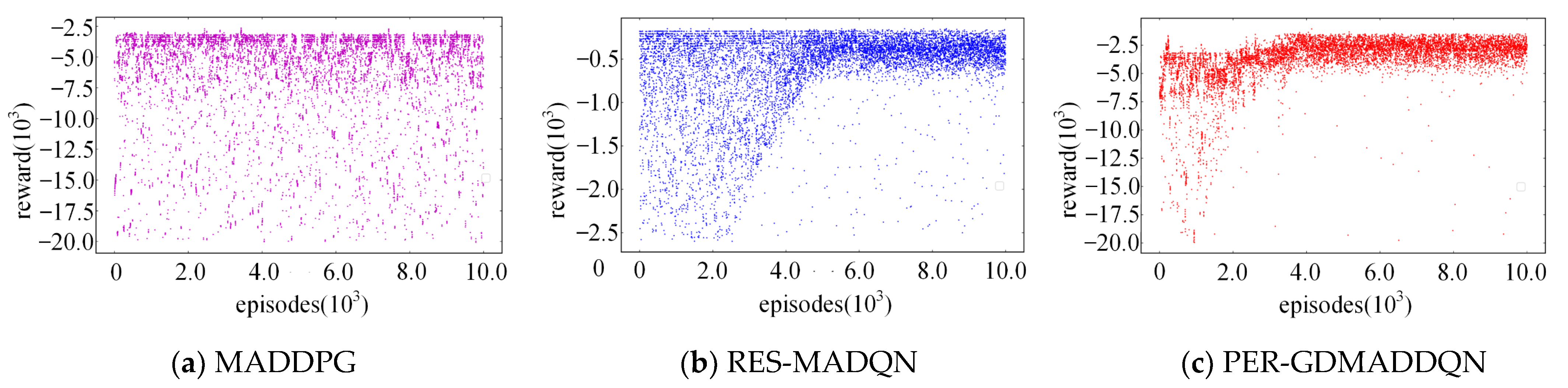
Convergence	No convergence trend after 10,000 episodes	Convergence after 6000 episodes	Convergence after 2000 episodes
Time-consumption	Unconverted	7169 s	5026 s
Average reward	Unconverted	−3500	−2600

. According to the results in Table 6, when compared with the MADDPG algorithm, the proposed algorithm is more suitable for path planning in a static environment. Compared with the RES-MADQN algorithm, the proposed algorithm significantly improves the solving efficiency and accelerates convergence.

5.3. Dynamic Target Pursuit

To further explore the performance of the proposed algorithm, the A* algorithm [41] is selected for comparison with the PER-GDMADDQN algorithm to carry out the pursuit task in a rasterized environment. The comparison results are shown in Figure 14.

As shown in Figure 14, both algorithms can successfully complete the pursuit task when the target moves. However, the PER-GDMADDQN algorithm has a shorter pursuit time, travels a shorter total distance, and has a smoother path. Specifically, in the early stage of the pursuit, all vehicles move towards the target. The difference is that the vehicles with the proposed algorithm can directly move along the diagonals of the grid, whilst the vehicles using the A* algorithm gradually move towards the target along orthogonal paths. The main reason is that the proposed algorithm in this paper expands the traditional four-direction output actions to eight-direction output actions, which not only improves the smoothness of the planned path but also greatly shortens it.

Table 7. Comparison of pursuit process data.

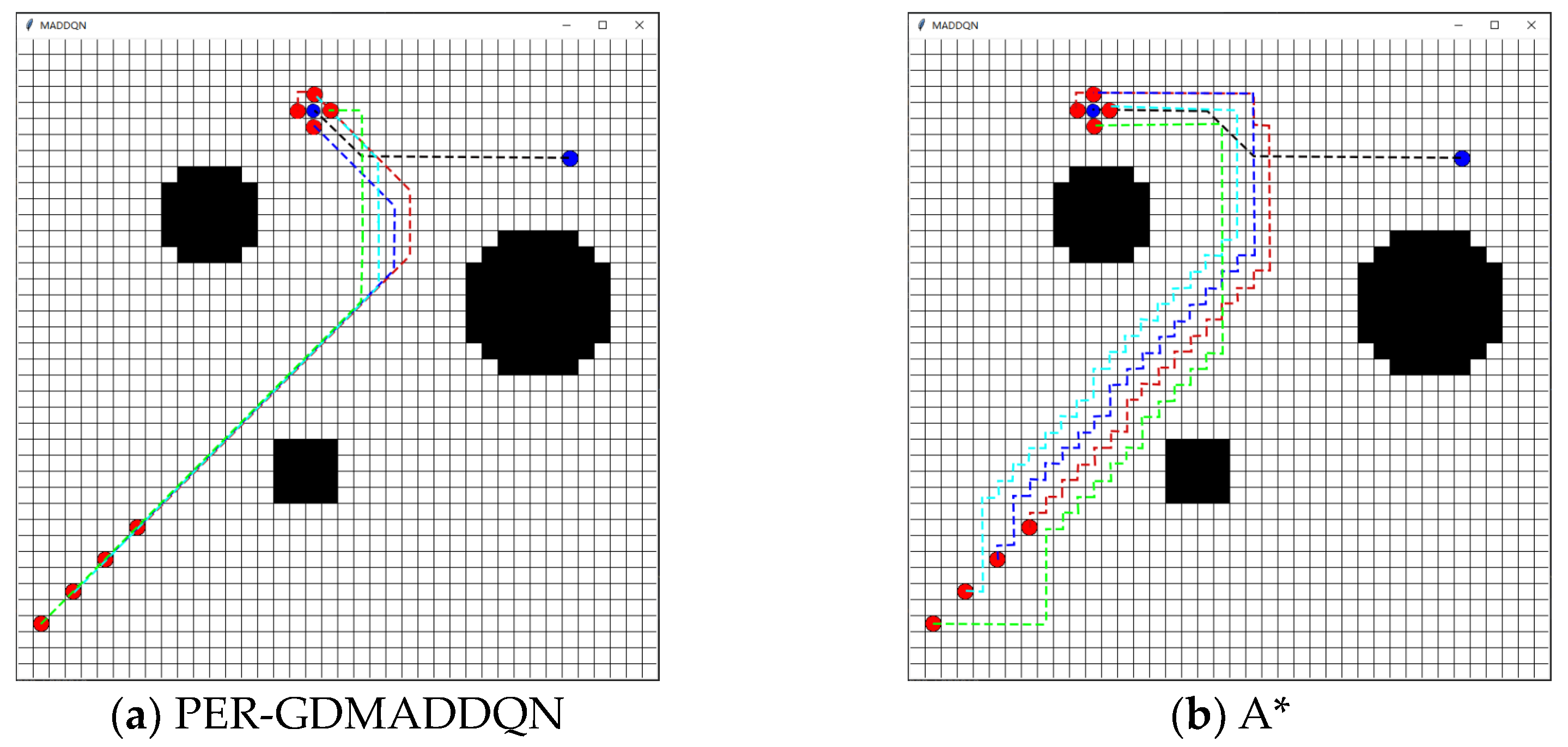
Parameter	PER-GDMADDQN	A*
Pursuit consuming (ms)	692	1933
Total path length	185	257

provides a statistical analysis of the pursuit indicator. The pursuit time indicates the duration of the entire process, from the moment the four unmanned vehicles start moving until the successful capture of the target. The total path length represents the combined distance calculated by all vehicles during the pursuit process. From Table 7, it can be noted that the proposed algorithm plans the pursuit path much faster than the A* algorithm, and its total path length is 28.02% shorter than that of the A* algorithm.

According to the analysis conducted in Table 7, it is evident that the proposed algorithm demonstrates efficient path planning during the testing phase. The time required for this process is approximately one-third of that required by the A* algorithm. This significant difference can primarily be attributed to the fact that the A* algorithm relies on a heuristic function to guide the search process and selects the optimal path using a priority queue. In contrast, the proposed algorithm utilizes a well-trained network that directly outputs the optimal strategy based on the input state value of the environment, thereby substantially reducing the planning time. Moreover, the total path length of the proposed method is reduced by 28.02% when compared to the A* algorithm. This reduction can be attributed to two factors. First, the proposed algorithm extends the action output and smooths the planned paths, greatly reducing the overall path length. Second, due to the reduced planning time, the movement distance of the target is shortened, naturally leading to a decrease in the tracking distance.

In order to enhance the fidelity of the simulation results and better reflect real-world application scenarios, the initial positions of the UGVs are randomized within a specific range ($x\in \left[\mathrm{0,8}\right], y\in \left[\mathrm{30,40}\right]$) in the simulation. The proposed algorithms are compared with MADDPG and RES-MADQN. Since the initial positions differ, this paper primarily focuses on comparing the average planning time and average reward based on the results of 100 tests, as depicted in Figure 15. The figure clearly demonstrates that, under the random initial position condition, the proposed method is superior to MADDPG and RES-MADQN in terms of path planning time and average reward.

To summarize, through comparisons with the MADDPG, RES-MADQN, and A* algorithms, the performance of PER-GDMADDQN is demonstrated. In the case of encircling static targets with multiple UAVs, all three algorithms can accomplish the pursuit task, while PER-GDMADDQN shows superior results. Additionally, when it comes to the pursuit of dynamic targets with multiple UAVs, PER-GDMADDQN significantly outperforms the A* algorithm.

6. Conclusions

In this study, we present a novel algorithm for path planning in multi-UGV pursuit scenarios. Specifically, our study investigates the challenges associated with multi-UGV pursuit and establishes a grid-based environmental model to address these challenges. We introduce the theoretical derivation of DDQN and extend it to the multi-UGV environment. Building upon this, we propose the PER-GDMADDQN algorithm, which incorporates gradient descent and a prioritized experience replay mechanism, which enables the UGVs to learn interactively in the grid environment and successfully complete the pursuit task. Simulation results demonstrate the effectiveness of the proposed algorithm, which outperforms other popular algorithms in terms of planning time and path smoothness.

While focusing on the pursuit of multiple UGVs in a 2D environment, it is important to acknowledge that real battlefield conditions are significantly more complex than the assumptions made in the proposed PER-GDMADDQN algorithm. Therefore, further investigations are required to explore the pursuit problem in 3D scenarios. Additionally, our study only considers a fixed number of UGVs pursuing a single target, neglecting the pursuit of multiple targets by varying numbers of UGVs. Future research should prioritize addressing this limitation and consider more complex scenarios.

References

- Fashey, H.K.M.; Miller, M.J. Unmanned Systems Integrated Roadmap Fiscal Year 2017–2042; United States Department of Defense: Washington, DC, USA, 2017. [Google Scholar]
- Liu, Y.; Jiang, C.; Zhang, T.; Zhao, Z.; Deng, Z. Multi-UAV finite-time ring formation control considering internal collision avoidance. J. Mech. Eng. 2022, 58, 61–68. [Google Scholar]
- Xu, C.; Zhu, H.; Zhu, H.; Wang, J.; Zhao, Q. Improved RRT*Algorithm for Automatic Charging Robot Obstacle Avoidance Path Planning in Complex Environments. Comput. Model. Eng. Sci. 2023, 12, 2567–2591. [Google Scholar] [CrossRef]
- Jiang, W.; Huang, R.; Zhao, Y. Research on cooperative capture method of USVs. In Proceedings of the 9th Academic Conference Professional, Beijing, China, 3–4 July 2021; pp. 45–50. [Google Scholar]
- Sang, H.; You, Y.; Sun, X.; Zhou, Y.; Liu, F. The hybrid path planning algorithm based on improved A* and artificial potential field for unmanned surface vehicle formations. Ocean Eng. 2021, 223, 108709. [Google Scholar] [CrossRef]
- Ding, H.; Cao, X.; Wang, Z.; Dhiman, G.; Hou, P.; Wang, J.; Li, A.; Hu, X. Velocity clamping-assisted adaptive salp swarm algorithm: Balance analysis and case studies. Math. Biosci. Eng. 2022, 19, 7756–7804. [Google Scholar] [CrossRef] [PubMed]
- Wang, Z.; Ding, H.; Yang, Z.; Li, B.; Guan, Z.; Bao, L. Rank-driven salp swarm algorithm with orthogonal opposition-based learning for global optimization. Appl. Intell. 2022, 52, 7922–7964. [Google Scholar] [CrossRef] [PubMed]
- Wang, Z.; Ding, H.; Yang, J.; Wang, J.; Li, B.; Yang, Z.; Hou, P. Advanced orthogonal opposition-based learning-driven dynamic salp swarm algorithm: Framework and case studies. IET Control Theory Appl. 2022, 16, 945–971. [Google Scholar] [CrossRef]
- Wang, Z.; Ding, H.; Wang, J.; Hou, P.; Li, A.; Yang, Z.; Hu, X. Adaptive guided salp swarm algorithm with velocity clamping mechanism for solving optimization problems. Comput. Des. Eng. 2022, 9, 2196–2234. [Google Scholar] [CrossRef]
- Sun, Y.; Lai, J.; Cao, L.; Chen, X.; Xu, Z.; Xu, Y. A Novel Multi-Agent Parallel-Critic Network Architecture for Cooperative-Competitive Reinforcement Learning. IEEE Access 2020, 8, 135605–135616. [Google Scholar] [CrossRef]
- Zhu, P.; Dai, W.; Yao, W.; Ma, J.C.; Lu, H.M. Multi-Robot Flocking Control Based on Deep Reinforcement Learning. IEEE Access 2020, 8, 150397–150406. [Google Scholar] [CrossRef]
- Wu, Z.; Hu, B. Swarm rounding up method of UAV based on situation cognition. J. Beijing Univ. Aero-Naut. Astronaut. 2021, 47, 424–430. [Google Scholar]
- Xu, C.; Zhang, Y.; Wang, W.; Dong, L. Pursuit and evasion strategy of a differential game based on deep reinforcement learning. Front. Bioeng. Biotechnol. 2022, 10, 827408. [Google Scholar] [CrossRef] [PubMed]
- Li, Q.; Lin, W.; Liu, Z.; Prorok, A. Message-Aware Graph Attention Networks for Large-Scale Multi-Robot Path Planning. IEEE Robot. Autom. Lett. 2021, 6, 5533–5540. [Google Scholar] [CrossRef]
- Fu, X.; Wang, H.; Xu, Z. Research on cooperative pursuit strategy for multi-UAVs based on de-maddpg algorithm. Acta Aeronaut. Et Astronaut. Sin. 2021, 43, 325311. [Google Scholar]
- Yuan, Z.; Wu, T.; Wang, Q.; Yang, Y.; Li, L.; Zhang, L. T3omvp: A transformer-based time and team reinforcement learning scheme for observation-constrained multi-vehicle pursuit in urban area. Electronics 2022, 11, 1339. [Google Scholar] [CrossRef]
- Wang, W.; Hao, J.; Wang, Y.; Taylor, M. Achieving cooperation through deep multiagent reinforcement learning in sequential prisoner’s dilemmas. In Proceedings of the First International Conference on Distributed Artificial Intelligence, Beijing, China, 13–15 October 2019; pp. 1–7. [Google Scholar]
- Mao, W.; Yang, L.F.; Zhang, K.; Başar, T. Decentralized Cooperative Multi-Agent Reinforcement Learning with Exploration. arXiv 2022, arXiv:2110.05707v2. [Google Scholar]
- Hartmann, G.; Shiller, Z.; Azaria, A. Competitive driving of autonomous vehicles. IEEE Access 2022, 10, 111772–111783. [Google Scholar] [CrossRef]
- Lowe, R.; Wu, Y.; Tamar, A.; Harb, J.; Abbeel, P.; Mordatch, I. Multi-agent actor-critic for mixed cooperative-competitive environments. In Proceedings of the Advances in Neural Information Processing Systems (NIPS 2017), Long Beach, CA, USA, 4–9 December 2017; pp. 1–16. [Google Scholar]
- Gong, T.; Yu, Y.; Song, J. Path Planning for Multiple Unmanned Vehicles (MUVs) Formation Shape Generation Based on Dual RRT Optimization. Actuators 2022, 11, 190. [Google Scholar] [CrossRef]
- Zhun, F.; Fuzan, S.; Peili, M.; Wenji, L.; Ze, S.; Zhaojun, W.; Guijie, Z.; Ke, L.; Bin, X. Stigmergy-based swarm robots for target search and trapping. Trans. Beijing Inst. Technol. 2022, 42, 158–167. [Google Scholar]
- González-Sierra, J.; Flores-Montes, D.; Hernandez-Martinez, E.G.; Fernández-Anaya, G.; Paniagua-Contro, P. Robust circumnavigation of a heterogeneous multi-agent system. Auton. Robot. 2021, 45, 265–281. [Google Scholar] [CrossRef]
- Moorthy, S.; Joo, Y.H. Distributed leader-following formation control for multiple nonholonomic mobile robots via bioinspired neurodynamic approach. Neurocomputing 2022, 492, 308–321. [Google Scholar] [CrossRef]
- Huang, H.; Kang, Y.; Wang, X.; Zhang, Y. Multi-robot collision avoidance based on buffered voronoi diagram. In Proceedings of the 2022 International Conference on Machine Learning and Knowledge Engineering (MLKE), Guilin, China, 25–27 February 2022; pp. 227–235. [Google Scholar]
- Kopacz, A.; Csató, L.; Chira, C. Evaluating cooperative-competitive dynamics with deep Q-learning. Neurocomputing 2023, 550, 126507. [Google Scholar] [CrossRef]
- Wan, K.; Wu, D.; Zhai, Y.; Li, B.; Gao, X.; Hu, Z. An improved approach towards multi-agent pursuit-evasion game decision-making using deep reinforcement learning. Entropy 2021, 23, 1433. [Google Scholar] [CrossRef]
- Wen, S.; Wen, Z.; Zhang, D.; Zhang, H.; Wang, T. A multi-robot path-planning algorithm for autonomous navigation using meta-reinforcement learning based on transfer learning. Appl. Soft Comput. 2021, 110, 107605. [Google Scholar] [CrossRef]
- De Souza, C.; Newbury, R.; Cosgun, A.; Castillo, P.; Vidolov, B.; Kuli, D. Decentralized multi-agent pursuit using deep reinforcement learning. IEEE Robot. Autom. Lett. 2021, 6, 4552–4559. [Google Scholar] [CrossRef]
- Xue, X.; Li, Z.; Zhang, D.; Yan, Y. A Deep Reinforcement Learning Method for Mobile Robot Collision Avoidance based on Double DQN. In Proceedings of the 2019 IEEE 28th International Symposium on Industrial Electronics (ISIE), Vancouver, BC, Canada, 12–14 June 2019; pp. 2131–2136. [Google Scholar]
- Zhang, R.; Zong, Q.; Zhang, X.; Dou, L.; Tian, B. Game of Drones: Multi-UAV Pursuit-Evasion Game With Online Motion Planning by Deep Reinforcement Learning. IEEE Trans. Neural Netw. Learn. Syst. 2023, 34, 7900–7909. [Google Scholar] [CrossRef] [PubMed]
- Parnichkun, M. Multiple Robots Path Planning based on Reinforcement Learning for Object Transportation. In Proceedings of the 2022 5th Artificial Intelligence and Cloud Computing Conference, Osaka, Japan, 17–19 December 2022. [Google Scholar] [CrossRef]
- Longa, M.E.; Tsourdos, A.; Inalhan, G. Swarm Intelligence in Cooperative Environments: N-Step Dynamic Tree Search Algorithm Extended Analysis. In Proceedings of the 2022 American Control Conference (ACC), Atlanta, GA, USA, 8–10 June 2022. [Google Scholar]
- Yu, Y.; Liu, Y.; Wang, J.; Noguchi, N.; Hea, Y. Obstacle avoidance method based on double DQN for agricultural robots. Comput. Electron. Agric. 2023, 204, 107546. [Google Scholar] [CrossRef]
- Liu, B.; Ye, X.; Dong, X.; Ni, L. Branching improved Deep Q Networks for solving pursuit-evasion strategy solution of spacecraft. J. Ind. Manag. Optim. 2022, 18, 1223–1245. [Google Scholar] [CrossRef]
- Dang, F.; Chen, D.; Chen, J.; Li, Z. Event-Triggered Model Predictive Control with Deep Reinforcement Learning for Autonomous Driving. arXiv 2022, arXiv:2208.10302. [Google Scholar] [CrossRef]
- Huang, L.; Hong, Q.; Peng, J.; Liu, X.; Zhen, F. A Novel Coordinated Path Planning Method using k-degree Smoothing for Multi-UAVs. Appl. Soft Comput. 2016, 48, 182–192. [Google Scholar] [CrossRef]
- Dian, S.; Zhong, J.; Guo, B.; Liu, J.; Guo, R. A smooth path planning method for mobile robot using a BES-incorporated modified QPSO algorithm. Expert Syst. Appl. 2022, 208, 118256. [Google Scholar] [CrossRef]
- Song, B.; Wang, Z.; Zou, L. An improved PSO algorithm for smooth path planning of mobile robots using continuous high-degree Bezier curve. Appl. Soft Comput. 2021, 100, 106960. [Google Scholar] [CrossRef]
- Pan, L.; Rashid, T.; Peng, B.; Huang, L.; Whiteson, S. Regularized softmax deep multi-agent q-learning. In Proceedings of the 35th Conference on Neural Information Processing Systems (NeurIPS 2021), New Orleans, LA, USA, 6–14 December 2021. [Google Scholar]
- Dang, C.V.; Ahn, H.; Lee, D.S.; Lee, S.C. Improved Analytic Expansions in Hybrid A-Star Path Planning for Non-Holonomic Robots. Appl. Sci. 2022, 12, 5999. [Google Scholar] [CrossRef]