Throughput Optimization for Blockchain System with Dynamic Sharding ^†

Abstract

Sharding technology, which divides a network into multiple disjoint groups so that transactions can be processed in parallel, is applied to blockchain systems as a promising solution to improve Transactions Per Second (TPS). This paper considers the Optimal Blockchain Sharding (OBCS) problem as a Markov Decision Process (MDP) where the decision variables are the number of shards, block size and block interval. Previous works solved the OBCS problem via Deep Reinforcement Learning (DRL)-based methods, where the action space must be discretized to increase processability. However, the discretization degrades the quality of the solution since the optimal solution usually lies between discrete values. In this paper, we treat the block size and block interval as continuous decision variables and provide dynamic sharding strategies based on them. The Branching Dueling Q-Network Blockchain Sharding (BDQBS) algorithm is designed for discrete action spaces. Compared with traditional DRL algorithms, the BDQBS overcomes the drawbacks of high action space dimensions and difficulty in training neural networks. And it improves the performance of the blockchain system by 1.25 times. We also propose a sharding control algorithm based on the Parameterized Deep Q-Networks (P-DQN) algorithm, i.e., the Parameterized Deep Q-Networks Blockchain Sharding (P-DQNBS) algorithm, to efficiently handle the discrete–continuous hybrid action space without the scalability issues. Also, the method can effectively improve the TPS by up to $28\%$.

1. Introduction

In recent years, blockchain technology has emerged as a disruptive and transformational technology with high trust and security potential, and it has been widely used in various fields, such as identity management [1], supply chains [2], game systems [3], food tracing [4], value trading [5], etc. However, it is still challenging to apply blockchain systems in large-scale systems because of their slow data-processing speed. For example, Ethereum [6] can encompass thousands of blockchain nodes, but it can only process 14 Transactions Per Second (TPS); Hyperledger [7] achieves throughput of more than 3500 TPS. However, in some industries such as finance, the TPS of 3500 is still too low to process a large number of transactions.

At present, the most effective way to improve blockchain throughput is to apply sharding technology to a blockchain and redesign its architecture. Sharding splits the blockchain network into multiple disjointed networks called shards. In a so-called shard network, each node only communicates with a limited number of nodes within the same shard. This technique substantially reduces the storage, computation and communication cost [8]. At present, extensive research is being conducted, both in academia and the industry, to optimize sharding policies to improve blockchain TPS. Sharding policies fall under either of the following two categories: (i) static and (ii) dynamic. Static methods refer to unchanged sharding policies [9,10,11,12]. Dynamic sharding technology can provide dynamic sharding strategies for dynamic blockchain environments, improving blockchain throughput. Yun et al. [13] proposed a Deep Q-Networks enabled Shard-based Blockchain (DQNBS) scheme that dynamically selects the optimal configuration (i.e., the number of shards, block size and block intervals, etc.) to maximize TPS. Zhang et al. [14] proposed SkyChain, which consists of an adaptive ledger protocol to facilitate merging or spliting the block, and an optimization framework which can adjust the number of shards, the block size and block interval for a long-term balance between security and TPS. However, their works may yield sub-optimal solutions since the action space is discrete and the number of available actions is strictly limited for tractability. This is because the Deep Q-Network (DQN) algorithm did not solve the problem of action space explosion, resulting in difficulty in training neural networks.

In the blockchain computing process, tasks need to be sharded in real time according to the resources and system conditions, i.e., the state at that time, so as to improve the execution efficiency of the system. This is consistent with the logic of MDP in dealing with the dynamic planning problem. Therefore, we endeavor to find higher-quality sharding polices by reformulating the Optimal Blockchain Sharding (OBCS) problem into a Markov Decision Process (MDP) with discrete–continuous hybrid action space, where the number of shards is discrete-valued, while the block size and block interval are continuous. We use two different methods to solve this problem. In the first method, we discretize continuous variables and then process them according to the discretization method. The Branching Dueling Q-Network (BDQ) algorithm is used in the blockchain fragmentation problem, and we propose the Branching Dueling Q-Network Blockchain Sharding (BDQBS) algorithm. The BDQBS solves the problem of action space explosion and provides better action strategies for blockchain systems, thereby improving blockchain performance. However, the BDQBS discretizes continuous action to obtain discrete action space, which ignores precise action. So, we used another method, applying the Parameterized Deep Q-Networks (P-DQN) algorithm to solve the problem in the discrete–continuous hybrid action space and propose the Parameterized Deep Q-Networks Blockchain Sharding (P-DQNBS) algorithm. The P-DQNBS provides more precise action strategies for blockchain systems, further improving the performance of blockchain.

The main contributions of this project are summarized as follows:

• Algorithm design: The BDQBS and P-DQNBS are proposed for blockchain sharding problems. Through the unique neural network structure of BDQ, BDQBS reduces the output dimension of the neural network, solving the problem of neural networks being difficult to train as a result of action space explosion. At the same time, it also shortens the time for parameter tuning and provides a fast sharding policy for blockchain. Compared to the BDQBS, the P-DQNBS provides a more accurate sharding policy for blockchain, which is more suitable for the real dynamic blockchain environment.
• Extensive simulation-based evaluation: We use Python to build a blockchain sharding simulation environment based on existing blockchain sharding systems. We implemented BDQBS and P-DQNBS for different action spaces in the optimization of blockchain throughput based on sharding technology. By comparing throughput, average sub-action and security, the results show that the BDQBS and P-DQNBS are significantly superior to the baseline algorithm. P-DQN and BDQ have increased throughput by 1.28 and 1.25 times.

The rest of the paper is organized as follows. Section 2 reviews the related literature. In Section 3, the system model is presented. Our proposed sharding algorithm is presented in Section 4, followed by simulation results in Section 5. Finally, we conclude this paper in Section 6.

2. Related Work

This section reviews related studies on sharding technology, which are grouped into two categories: static sharding and dynamic sharding. Traditional blockchain networks usually use static sharding to process transactions, i.e., the entire network is divided into multiple fixed-size blocks, each of which processes a certain number of transactions. The static sharding process is relatively simple and easy to implement. However, static sharding is prone to network congestion and transaction latency problems. Dynamic sharding dynamically adjusts the size and number of shards based on the network load and the node availability, ensuring that the network is always able to handle highly concurrent transactions. Dynamic sharding is complicated to implement due to the complexity of parameter changes.

2.1. Static Sharding Technology

Typical static sharding techniques are Elastico [9] and OmniLedger [10]. Lu et al. [9] proposed Elastico, the first sharding technology for public chains, which combines the Proof of Work (PoW) [15] protocol with the Practical Byzantine Fault Toll (PBFT) [16,17] protocol. Nodes establish identification through PoW first, and then are randomly assigned to various committees. A committee can complete the PBFT protocol in each step as the number of nodes in each committee is small enough. Thus, the nodes in each committee can process transactions in parallel, which almost achieves linear scaling of throughput. However, Elastico cannot handle cross-sharding transactions.

The overall architecture of OmniLedger [10] is composed of one identity chain and multiple subchains. OmniLedger uses the RandHound [18] protocol to divide all nodes into different groups and randomly assign these groups to different sharding subchains. The consensus within each shard adopts the PBFT protocol. By removing the full sequence requirements of the blocks, OmniLedger organizes the blocks into a Directed Acyclic Graph structure, which increases the system throughput and reduces the transaction confirmation delay. In addition, OmniLedger uses atomic submission protocols to handle cross-sharding transactions. And by using ledger-editing technology, it sets checkpoints and prunes historical data before checkpoints to reduce the storage pressure on nodes. Using OminiLedger, the throughput of the blockchain increases linearly with the number of shards.

Based on Elastico and OmniLedger, researchers have made improvements to blockchain system architectures, such as Zilliqa [11] and Rapid Chain [12]. The Zilliqa team conducted architecture and performance optimization based on Elastico. In terms of architecture, they proposed a dual-chain architecture, with one transaction chain storing transaction data and one directory service chain storing miner metadata information. In terms of performance optimization, Zilliqa adopted CoSi multi-signature technology in the consensus phase. By using digital signatures instead of MAC in the PBFT protocl, the PBFT can be applied to hundreds of nodes, greatly improving its scalability. On the basis of OmniLedger, RapidChain [12] added information distribution technology based on erasure codes to accelerate the propagation speed of blocks, achieving full sharding technology covering communication computation and storage. In order to reduce the state cost, RapidChain adopts the Cuckoo protocol, which only needs to replace some nodes during each sharding switch. The RapidChain system mainly consists of three important phases, namely the bootstrapping phase, consensus phase and reconfiguration phase. The bootstrapping phase will only run once at the beginning of the RapidChain system, creating an initial random source and randomly selecting a special committee called the reference committee, whose members randomly allocate nodes to form a sharding committee.

2.2. Dynamic Sharding Technology

Although the static methods are easy to design and implement, they cannot adapt to the dynamic blockchain environment, such as a variation in the number nodes in the system and intermittent attacks from malicious nodes, etc. Dynamic sharding technology solves the problem that the sharding policy cannot be adjusted according to the situation. To address this issue, a popular approach is to formulate the OBCS problem as a Markov Decision Process (MDP) and integrate DRL into the sharding controller.

Yun et al. [13] proposed a scalable blockchain system based on fragmentation, which optimizes throughput while maintaining a high security level. They combined sharding technology with DRL, abstracted the blockchain sharding selection process into the MDP and proposed the DQNBS method. Sharding technology continuously delegates mining tasks to other nodes. By adjusting the number of shards, the security level can be changed proactively. It uses DRL to optimize the performance of the blockchain to meet large-scale and dynamic Internet of Things operations. In particular, based on the DRL framework, the concept of trust is integrated into the consensus phase. Thus, we can estimate the malicious probability of the network by monitoring the consensus result of each epoch. Based on network trust, the blockchain calculates the number of secure shards and adopts adaptive control to maintain optimal throughput conditions.

Zhang et al. [14] proposed a sky chain which combines blockchain with DRL. This is a new type of blockchain framework based on dynamic sharding, which achieves a balance between performance and security without affecting scalability in dynamic environments. Firstly, the sky chain adopts an adaptive ledger protocol to ensure that the ledger based on dynamic fragmentation policy can be effectively consolidated or split. Then, it proposes a fragmentation method based on DRL in order to optimize the fragmentation policy under the dynamic environment of a high-dimensional system state. The authors constructed a framework to evaluate blockchain sharding systems in terms of performance and security, achieving a long-term balance between the two by adjusting the sharding interval, number of shards and the block size. In addition, DRL can learn the characteristics of the system from previous experience and obtain long-term returns by adopting appropriate fragmentation strategies according to the current network state.

The above dynamic sharding technologies based on DRL generally adopts the basic DRL algorithm DQN, which solves the problem of state space explosion. However, when the action dimension increases and leads to an explosion in the action space, using DQN will result in the inability of neural network training.

3. System Overview

3.1. System Model

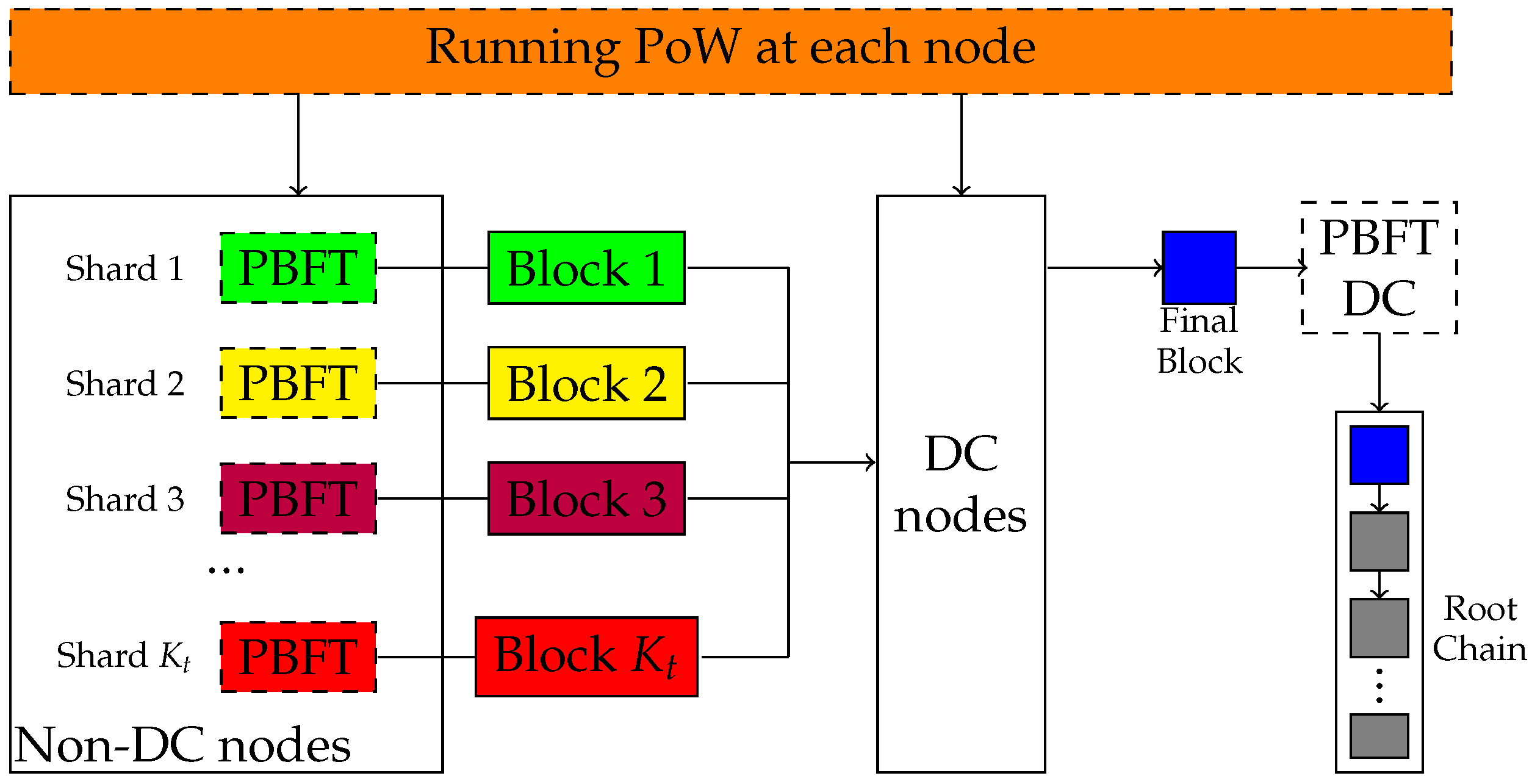
The blockchain sharding system containing N nodes is shown in Figure 1. The blockchain sharding system divides nodes into different shards, and nodes within the shards process transactions in parallel. Firstly, each node in the blockchain needs to solve a workload problem, PoW, to obtain its own identity (ID). The calculation process involves putting the “seed” of the PoW (i.e., EpochRand), the IP address, public key (PK) and the random number Nonce through the SHA-256 hash algorithm to obtain ID. The ID needs to be smaller than the target difficulty value d in the blockchain; i.e., the ID is a 256-bit value that starts with a certain number of 0 bits. Since the SHA-256 hash algorithm is irreversible, the only way to compute the hash value is that the node needs to keep trying to input different values of Nonce until it finds a hash value that meets the conditions. This process consumes a lot of computational resources and time in order to ensure the security of the algorithm. Then, a certain number of nodes are selected form the directory committee (DC) based on the speed of resolving the PoW. Once the nodes in the DC are identified, the blockchain is sharded and the nodes in the blockchain are divided into K shards based on the node’s ID. The transactions are processed in parallel, and the nodes in the shards pack the transactions into blocks and execute the Practical Byzantine Fault Tolerance (PBFT) consensus algorithm. PBFT is used to solve the Byzantine Fault Tolerance problem in blockchain networks, i.e., how to guarantee the correctness of the consensus result in the presence of some malicious nodes in the network. The nodes in the shards verify the block and send it to the DC, which packages it into a final block, performs PBFT on it, uploads it to the blockchain after verification and returns the packaged information to all the nodes in the shards for updating.

At epoch t, the computing capability of node i is denoted as $C_{i,t}$. Sharding begins from each node using its computing capability $C_{i,t}$ to run a computational-intensive task knows as PoW to obtain the identity in the blockchain. All nodes are then grouped as DC nodes and non-DC nodes:

• DC nodes. DC nodes are those who solve the PoW first. They receive local blocks from each shard, and a randomly chosen primary DC node generates the final block by merging all local blocks. The final block should be validated by all DC nodes via PBFT consensus protocol before being broadcast throughout the network and linked to the root chain.
• Non-DC nodes. Non-DC nodes in the blockchain are divided into $K_t$ shards. Here we assume that a transaction can only be assigned to one shard, which is implemented in account-based sharding [20]. All shards process transactions in parallel and create local blocks of size $B_t$ at interval $T_t$. Then, nodes in a shard broadcast messages through the communication channel with transmission rate $R_{i,j,t}$ to perform a local PBFT consensus protocol to validate that the information in the local block is correct.

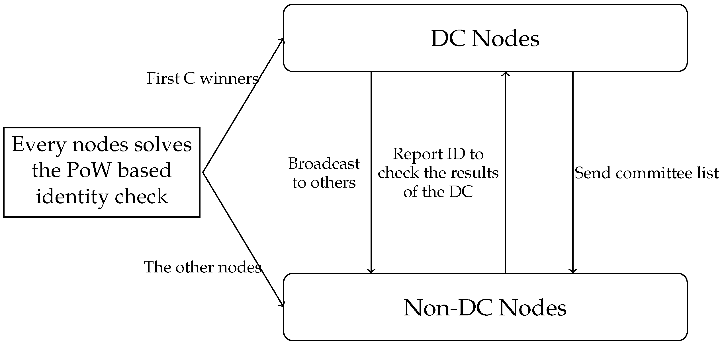
3.2. Blockchain Sharding Mechanism

The blockchain sharding clustering mechanism is shown in Figure 2. Firstly, each node selects its own PK and IP address locally for future authentication. Nodes in blockchain networks can obtain their own IDs by solving a simple PoW. The identity ID of q node can be represented as

$$ID=H(EpochRand||IP||PK||Nonce)<d,$$

(1)

where EpochRand is the “seed” of the PoW, which needs to be generated at the end of the previous epoch to ensure that the PoW is not pre-caculated. d is the difficulty level of the PoW algorithm. It is a predefined parameter in the network which determines how much computing power is needed to solve the PoW. H is a hash operation.

A sharded blockchain consists of a DC and K shards. To share the sharding information, we need to select DC nodes first. The nodes in the DC are composed of the top C nodes that solve the PoW the fastest. To ensure that the number of nodes in the DC is similar to the other K shards, C = $\lfloor N/[K+1]\rfloor$. After the nodes in the DC are determined, the information is broadcast to other nodes. The non-DC nodes will check the information of the DC nodes. Then, the nodes are assigned into shards, according to the last L bit of the node ID. For example, if $L=3$, the shard number is equal to the last three digits of ID, namely, $2^L=2^3=8$. All nodes need to send their own information, namely PK, EpochRand, Nonce and ID, to the DC. The nodes in the DC collect all the information and broadcast it throughout the entire network, enabling the entire network to receive fragment information. After each node knows its shard number, nodes within the same shard establish point-to-point connections.

After the blockchain shard is complete, the division of transactions is determined based on the account UTXO, which means that the transaction is allocated to the shard that matches the last L-bit hash value of the sender’s account. This is to prevent malicious users from generating transactions that exceed their balance and distributing them to different shards.

3.3. Markov Decision Process Formulation for Optimal Blockchain Sharding Problem

We model the blockchain sharding problem as an MDP. In our system, the state space, action space and reward function are defined as follows:

• State Space. The system state at epoch t can be expressed by

  $$s_t=[{\mathit{R}}_t,{\mathit{C}}_t,{\mathit{H}}_t,P_t],$$

  (2)

  where ${\mathit{R}}_t=\{R_{i,j,t}\}$ is the matrix of the data transmission rate, $i,j\in N$; ${\mathit{C}}_t=\{C_{i,t}\}$ is the vector of the node computing capability; $P_t$ is the probability of malicious nodes in the blockchain at time t, which is calculated based on consensus history [13]; and ${\mathit{H}}_t=\{H_{i,t}\}$ is the vector of the consensus history of the previous epoch slot, which is a binary variable where $H_{i,t}=0$ means that node i accepted the block to be linked to the blockchain at epoch $t-1$ and vice versa.
• Action Space. The throughput is closely related to the number of shards $K_t$, block size $B_t$ (in bytes) and block interval $T_t$. Thus, we define the action at epoch t as

  $$a_t=[K_t,B_t,T_t],$$

  (3)

  where $K_t$ is discrete and is selected from a finite enumerable set $\{1,2,\dots ,k_{max}\}$; $T_t\in [T_{min},T_{max}]$ is continuous. $B_t$ is also discrete, but since the action space of $B_t$ is quite large, e.g., several Megabytes, we assume that $B_t$ is approximately continuous.
• Reward Function. We use the transaction throughput as our reward function. The reward $r_t$ in epoch t can be defined as

  $$r_t=\left\{\begin{array}{ccc}\frac{K_t\times \lfloor (B_t-B_H)/b\rfloor }{T_t}\hfill & \hfill ,& \mathrm{constraints}\mathrm{C}1\text{–}\mathrm{C}3\mathrm{are}\mathrm{satisfied},\hfill \\ 0\hfill & \hfill ,& \mathrm{otherwise},\hfill \end{array}\right.$$

  (4)

  $$C1:k_{max}<(N[1-3P_t]-1)/[3N{P}_t+1]$$

  (5)

  $$C2:k_{max}<(2N/[3P_t+1])-1$$

  (6)

  $$C3:T_{latency}=T+T_c^k\le uT,K=1,2,\dots ,k$$

  (7)

  where the numerator is the number of transactions processed by $K_t$ shards in parallel and the denominator $T_t$ represents the block interval. $B_H$ is the size of the block head and b is the average size of transactions. In (4), constraints C1 and C2 are security constraints to ensure that after blockchain nodes are sharded, malicious nodes within the shard cannot threaten the security of the entire shard, and to prevent blocks generated by malicious nodes from being uploaded to the blockchain. Constraint C3 is a delay constraint. In order to meet the final attributes of the blockchain, the delay should be completed within several consecutive block intervals u. $T_c$ is the time consumed for consensus.

3.4. The Optimal Blockchain Sharding Problem

The optimal blockchain sharding problem can now be written as the following optimization problem:

$$\underset{a_t=[K_t,B_t,T_t]}{max}\mathbb{E}\sum _{t=0}^T{\gamma }^t{r}_t,$$

(8)

where $\gamma \in [0,1]$ is the discount rate.

Note that $P_t$ can be determined based on ${\mathit{H}}_t$, and $T_c$ depends upon $B_t$ and $K_t$. The details for calculating these variables can be found in [13], which we omit here due to space limitations. Problem (8) seeks to maximize the accumulated throughput. Given a policy $\pi$, which is a mapping between states and actions, the Q function is defined as the expectation of accumulated reward from state $s_t$ after executing action $a_t$ and following policy $\pi$, i.e.,

$$Q_{\pi }(s_t,a_t)={\mathbb{E}}_{\pi }\left[\sum _{\tau =0}^{\infty }{\gamma }^{\tau }{r}_{t+\tau }|s_t,a_t\right].$$

(9)

The optimal action can be selected once the optimal Q function is found. The optimal Q function satisfies the optimal Bellman equation defined as

$$Q_{\pi }^{\ast }(s_t,a_t)={\mathbb{E}}_{\pi }[r_t+\gamma \underset{a_{t+1}}{max}{Q}^{\ast }(s_{t+1},a_{t+1})].$$

(10)

The traditional Q learning algorithm learns the optimal Q function by

$$\begin{array}{cc}\hfill Q_{\pi }(s_t,a_t)& =Q_{\pi }(s_t,a_t)+\hfill \\ \hfill & \alpha (r+\gamma \underset{a_{t+1}}{max}{Q}_{\pi }(s_{t+1},a_{t+1})-Q_{\pi }(s_t,a_t)),\hfill \end{array}$$

(11)

where $\alpha \ge 0$ is the learning rate, and the Q function is stored in a lookup table. An issue with Q learning is that it can only solve MDPs with discrete action space. However, our problem has a discrete–continuous hybrid action space. As such, it is impossible to directly apply the Q learning algorithm to estimate the optimal Q function. In the next section, we leverage the BDQ and P-DQN [21] to solve problem (8).

4. The Blockchain Sharding Algorithm

In order to improve the performance of the blockchain sharding system, we proposes two blockchain sharding control algorithms based on DRL for different action spaces, namely, blockchain sharding algorithms based on BDQ and P-DQN. The blockchain sharding algorithm based on BDQ not only solves the problem of discrete action space explosion, but also solves the problem of neural networks being difficult to train as a result of action space explosion. The BDQ proposes a new neural network structure with a shared decision module, which is connected to the network branches and state value branches of subactions in the action space. Moreover, it provides a certain degree of independence for each individual action dimension and has better scalability. The blockchain sharding algorithm based on P-DQN solves the problem of discrete–continuous hybrid action space in blockchain sharding decision making. P-DQN uses two different neural networks, namely the policy network and the value network, to predict action. The policy network outputs the continuous action parameters corresponding to a given discrete action, and obtains the continuous action value function from the continuous action parameters and state input value network. The optimal action is selected based on the value function.

4.1. The BDQBS Algorithm

When using DRL to deal with blockchain sharding problems, most studies use DQN to provide the blockchain sharding policy. DQN solves the problem of state space explosion, but when dealing with the problem of action space explosion caused by the combination of the number of actions and the number of action dimensions, DQN has the drawbacks of a complex neural network output and difficulty in training. BDQ is an extension of DQN that proposes a new neural network structure to approximate multidimensional action space functions, achieving a linear increase in network outputs with degrees of freedom. It enables the better training of neural networks, resulting in better action strategies. Therefore, we use BDQ to find the optimal solution to the blockchain sharding problem in the discrete action space.

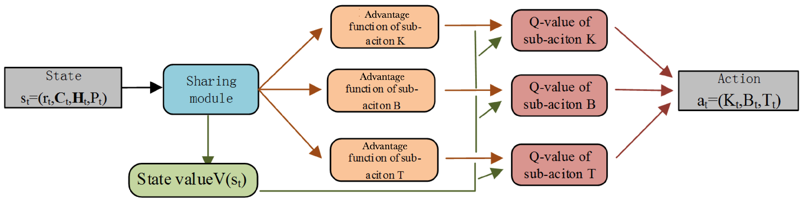
The neural network structure of BDQ is shown in Figure 3. The state $s_t=({\mathit{R}}_t,{\mathit{C}}_t,{\mathit{H}}_t,P_t,)$ is input into the neural network. After the shared module, it outputs the dominant functions of $K,B,T,A(s_t,K_t),A(s_t,B_t),A(s_t,T_t)$ and the state value function $V(s_t)$. The dominant function is added to the state value function to obtain the Q value, which is used to select the optimal action.

4.1.1. Algorithm Design

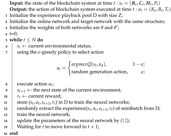
Algorithm 1 shows the details of our BDQ algorithm. In each epoch t, the algorithm first initializes the experience replay pool $\mathit{D}$ to store the experience samples generated by interactions between the agent and the blockchain environment. The experience samples are used to train the neural network. Two neural networks with the same structure, online network and target network, as well as weight $\theta$ and ${\theta }^{\prime }$, are initialized. The status of the blockchain environment $s_t=({\mathit{R}}_t,{\mathit{C}}_t,{\mathit{H}}_t,P_t)$ is obtained at the current time t (line 6). With the state $s_t$, the network outputs the advantage function $(A_K,A_B,A_T)$ and state value function $V(s_t)$ of the subaction and adds them together to obtain the Q value of the action. Select $a_t=(K_t,B_t,T_t)$ of blockchain sharding based on the $ϵ$-greedy policy [22] (line 7). Input $a_t$ into the blockchain (line 8). The blockchain nodes are divided into K shards based on $K_t$. According to $B_t$ and $T_t$, the node processes transactions in parallel within time t and generates a block of size B. The DC collects the blocks generated by sharding, merges them into final blocks, and uploads them into the blockchain. The blockchain system proceeds to the next state $s_{t+1}=({\mathit{R}}_{t+1},{\mathit{C}}_{t+1},{\mathit{H}}_{t+1},P_{t+1})$ and obtains reward $r_t$, i.e., the throughput of processing transactions (line 9–10). The samples generated by the interaction between the agent and the blockchain system environment are stored in the experience pool to update the neural network (line 11). At last, the network is trained by the experience extracted from experience pool D and the parameters are updated (line 12).   

Algorithm 1: The BDQBS Algorithm process

4.1.2. Approximation Architecture

According to Figure 3, the specific steps for updating the neural network parameters in line 8 of Algorithm 1 are as follows. The output of the BDQ neural network consists of the advantage function and state values of multiple action branches. The Q value of the action is obtained by adding the advantage function to the state value. According to (12), the loss values are calculated based on each Q value of multi-actions and the target function, respectively. They are added together to obtain the final loss value.The gradient descent method is used to update neural network parameters. The green arrows represent the flow of the state value, and the red arrows represent the function computation process for the sub-actions.

$$L=E_{s_t,a_t,R_{t+1},s_{t+1}D}[\frac{1}{N}\sum _d{(y_d-Q_d(s_t,a_d))}^2]$$

(12)

where $y_d$ is defined as

$$y_d=r+\gamma \frac{1}{N}\sum _d\underset{a_d^{\prime }\in A_d}{Q_d^{\prime }(s_{t+1},argmax{Q}_d(s_{t+1},a_d))}$$

(13)

$\underset{a_d^{\prime }\in A_d}{Q_d^{\prime }(s_{t+1},argmax{Q}_d(s_{t+1},a_d))}$ obtains the Q value based on the state–action pair in the $Q_d^{\prime }$ network, and the sub-action $a_d$ is determined by the maximum Q value based on the state $s_{t+1}$ in the $Q_d$ network. The Q function in (14) consists of the state value function $V(s_t)$ and the advantage function $A_d(s_t,a_d)$.

$$Q_d(s_t,a_d)=V(s_t)+A_d(s_t,a_d)$$

(14)

There are two neural networks with the same structure in the algorithm, where the online network updates in real-time and the target network is updated every C steps, using the parameters of online network.

4.2. The P-DQNBS Algorithm

In the real blockchain, the number of shards and the block size are discrete parameters. However, due to the large action space of the block size, such as $[0,2^{23}]$, we approximately assume that the block size and block interval are continuous. Furthermore, the block size and block interval in the action space of the blockchain sharding problem can be regarded as continuous decision variables to construct a mixed-action-space MDP, further reducing the discrete action space. For the processing of mixed action spaces, previous work has approached the discrete action space by discretizing continuous action or relaxing discrete action into a continuous set to obtain a continuous action space. We used the P-DQN framework to solve the mixed action space problem and provide more accurate action for sharded blockchain networks. The P-DQN algorithm seamlessly integrates DQN for discrete action and Deep Deterministic Policy Gradient [23] for continuous action.

4.2.1. Algorithm Design

Algorithm 2 shows the details of our P-DQNBS algorithm. In each epoch t, it first computes the optimal continuous action $B_{K_t}^{\ast }$ and $T_{K_t}^{\ast }$ for each $K_t\in \{1,2,\dots ,k_{max}\}$ based on the current state $s_t$ (line 5), then selects the optimal $K_t^{\ast }$ by

$$K_t^{\ast }=arg\underset{K_t\in \{1,2,\dots ,k_{max}\}}{max}Q(s_t,K_t,B_{K_t}^{\ast },T_{K_t}^{\ast };\omega )$$

(15)

and obtains the optimal action $a_t^{\ast }=[K_t^{\ast },B_{K_t^{\ast }}^{\ast },T_{K_t^{*}}^{*}]$ (lines 6–7). Then, an action chosen from the $ϵ$-greedy policy

$$a_t=\left\{\begin{array}{c}\mathrm{A} \mathrm{random} \mathrm{action}, \mathrm{with} \mathrm{probability} ϵ,\hfill \\ [K_t^{\ast },B_{K_t^{\ast }}^{\ast },T_{K_t^{\ast }}^{\ast }], \mathrm{otherwise}.\hfill \end{array}\right.$$

(16)

is executed (line 8). The reward can be computed by (4) (line 9) since violation of constraint C1–C2 indicates that the ratio of malicious nodes is greater than the upper bound required by the PBFT consensus protocol, and consequently, no block is generated. Violation of constraint C3 means that the block cannot be verified within the threshold, which means the uploading of the block to the blockchain fails. Next, a system transition $(s_t,a_t,r_t,s_{t+1})$ is formed and stored in the replay buffer $\mathcal{D}$ (line 10), from which a minibatch $\mathcal{M}$ is sampled to train the policy network and value network, respectively (line 11). More specifically, the policy network is updated by maximizing the Q function; therefore, the loss function is set as

$${\mathcal{L}}_t^{\mathsf{\Theta }}(\theta )=\sum _{(s_{\tau },a_{\tau },r_{\tau },s_{\tau +1})\in \mathcal{M}}Q(s_{\tau },K_{\tau },B_{K_{\tau }}^{\ast },T_{K_{\tau }}^{\ast };\omega )$$

(17)

(line 9). The updating target for the value network is

$$y_{\tau }=r_{\tau }+\underset{K_{\tau +1}\in \{1,2,\dots ,k_{max}\}}{max}\gamma Q(s_{\tau },K_{\tau },B_{K_{\tau }}^{\ast },T_{K_{\tau }}^{\ast };\omega )$$

(18)

and is updated by minimizing the squared TD error, i.e.,

$${\mathcal{L}}_t^Q(\omega )=\frac{1}{2}\sum _{(s_{\tau },a_{\tau },r_{\tau },s_{\tau +1})\in \mathcal{M}}{[Q(s_{\tau },K_{\tau },B_{K_{\tau }}^{\ast },T_{K_{\tau }}^{\ast };\omega )-y_{\tau }]}^2$$

(19)

(lines 13–14).

In order to enhance the stability of P-DQNBS, we also use the target networks [24], which are periodically updated (line 15).

Algorithm 2: The P-DQNBS Algorithm process

4.2.2. Approximation Architecture

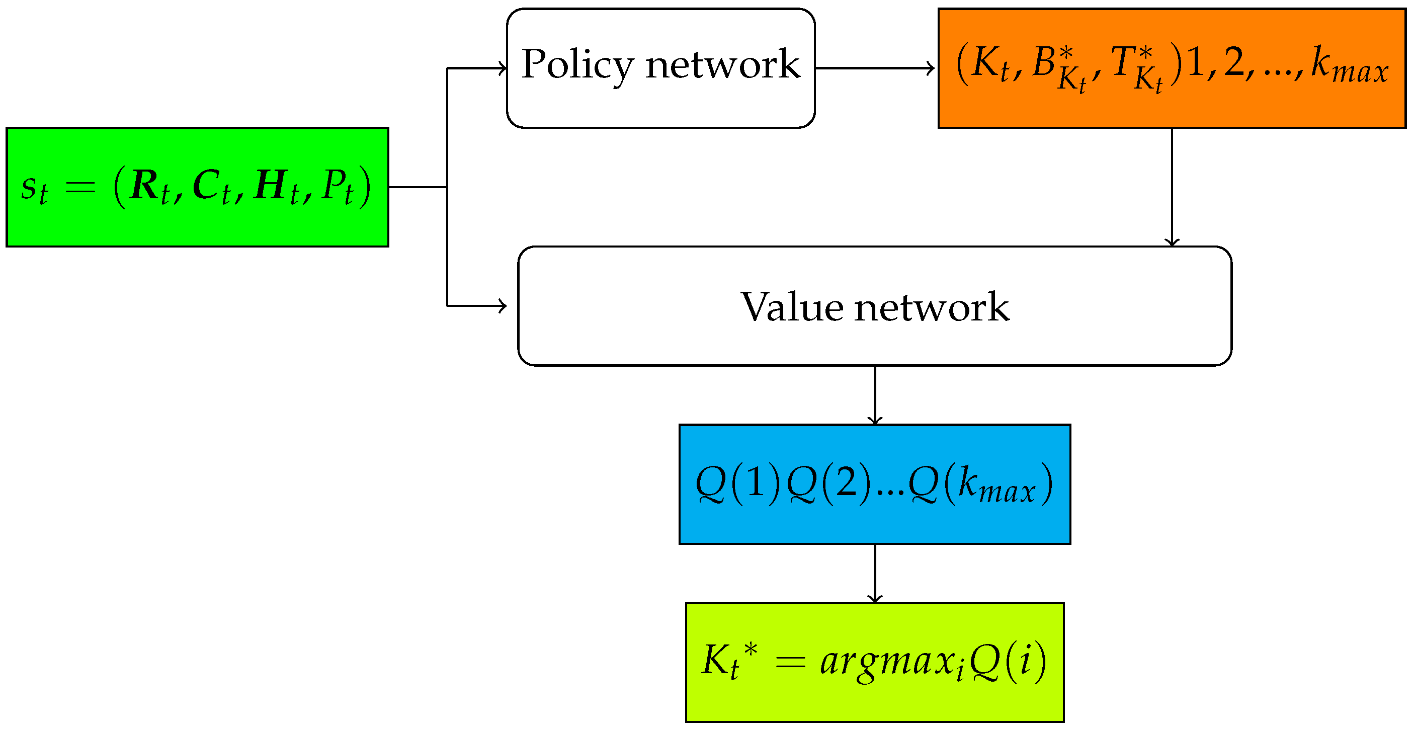
To improve the algorithm’s scalability, we use a neural network shown in Figure 4 to approximate the Q function. The neural network consists of two components, i.e., a policy network and a value network. The policy network parameterized by $\theta$ takes the system state $s_t$ as input, and outputs $B_{K_t}^{\ast }$ and $T_{K_t}^{\ast }$, i.e., the optimal continuous actions with regard to a particular discrete action $K_t$; the value network parameterized by $\omega$ takes the system state $s_t$, $B_{K_t}^{\ast }$ and $T_{K_t}^{\ast }$ as input and outputs $Q(s_t,K_t,B_{K_t}^{\ast },T_{K_t}^{\ast };\omega )$ of each discrete action $K_t\in \{1,2,\dots ,k_{max}\}$.

The training of the policy network and value network by our Parameterized Deep Q-Networks Blockchain Sharding (P-DQNBS) algorithm is shown in detail as follows.

5. Simulations

In order to ensure the validity of the research findings, we used Python to build a blockchain simulation environment based on the fragmentation process of the blockchain system to simulate the actual sharding computation process. We used the Pytorch framework to implement the DRL. The proposed algorithms are implemented in the simulation environment to simulate the operation of algorithms under real conditions. Finally, we compared our algorithms with other algorithms under the same environmental parameters to obtain quantitative results. The interaction flowchart between the blockchain simulation environment and the algorithm is shown in Figure 5.

After initialization, the transmission rate, computing power, consensus history and probability of malicious nodes between nodes in the blockchain at the current time are taken as the system state $s_t$. The state $s_t$ is input into the neural network of the algorithm, and a random action or neural network action is selected through $ϵ$-greedy strategy is output as action $a_t$. Subsequently, the system enters the next moment $s_{t+1}$ and calculates the immediate reward $r_t$. The experience ($s_t$, $a_t$, $r_t$, $s_{t+1}$) is stored in the experience pool. And the batch size of experience is selected to update the neural network parameters. All data are seaved and $s_{t+1}$ is set as the current state $s_t$ to start the next cycle.

5.1. Parameter Settings

This section mainly describes the setting of experimental environment parameters, as well as BDQBS and P-DQNBS parameters. Due to the different neural network structures of the two algorithms, the parameter settings are based on the experimental results of tuning the parameters of each algorithm.

5.1.1. Parameters for the Blockchain Environment

We use PyTorch [25] to build neural networks and implement our proposed algorithm with Python 3.6. The simulation environment is the same as [13], which includes 200 nodes. The maximum number of shards is 8. The maximum block interval and maximum block size are set to 16 s and 8 MB. The average transaction size and block header size are assumed to be 200 B and 80 B. The computing capability and data transmission rate follow uniform distributions. The policy network has three hidden layers, with the number of neurons being 256, 128 and 64, respectively; the value network has two hidden layers, with the number of neurons being 128 and 64, respectively. The policy network and value network use Adam optimization.

Table 1. Parameters for the blockchain environment.

Symbol	Parameters	Value
N	Number of nodes	200
$k_{max}$	Maximum allowable shard number	8
$T_{max}$	Maximum block interval	16 s
$B_{max}$	Maximum block size of each shard	8 MB
b	Average transaction size	200 Bytes
$B_H$	Block header size	80 Bytes
$C_{i,t}$	Computing capability of node i at epoch t	10–30 GHz
$R_{ij,t}$	Data transmission rate between node i and j at epoch t	10–100 Mbps

summarizes the parameter settings used in this paper.

5.1.2. Parameters for the Algorithms

As the Q-function is unknown, we incorporate neural networks in the reinforcement learning process, using the basic neural network Back Propagation for function approximation. For the BDQBS and P-DQNBS algorithm, we use the following settings. We set the number of neurons in the hidden layer to 256, 128 and 64, respectively. The discount factor $\gamma$ is set to 0.9 to make the algorithms more inclined towards long-term optimization, which is beneficial for maximizing rewards. In order to explore better action in the early stage of the algorithms, the initial exploration probability of the algorithms is set to 0.9. After the algorithms explore 2000 steps, the exploration probability decreases by 0.01 per step until the exploration probability reaches 0.1. We set the experience pool size to 1000 and the update frequency of neural network parameters to update every 10 steps.

We set the number of hidden layers in the BDQBS algorithm neural network to 3, and set the learning rate r to 0.05. The number of experiences selected when updating the neural network is 32. In addition, dropout was introduced to prevent overfitting of the neural network, with a random inactivation ratio of 0.5.

The neural network of the P-DQNBS algorithm consists of a policy network and a value network. The number of hidden layers in both networks is set to 3. We set the learning rate $r_p$ of the policy network to 0.001, and the learning rate $r_v$ of the value network to 0.0001. We select 128 experiences when updating the neural network.

Table 2. Parameters for BDQ and PDQ algorithm neural network.

Algorithm	Symbol	Parameters	Value
BDQBS	r	Neural network learning rate	0.05
	M	Number of experiences extracted	32
	$\delta$	Random inactivation rate of neural networks	0.5
P-DQNBS	$r_p$	Policy network learning rate	0.05
	$r_v$	Value network learning rate	0.05
	M	Number of experiences extracted	32

shows the differences between the BDQBS and P-DQNBS settings.

5.2. Performance Comparison

We compared DQNBS as a baseline algorithm with our proposed P-DQNBS and BDQBS. The advantages and disadvantages of the three algorithms are shown in

Table 3. Comparison of algorithm advantages and disadvantages.

Algorithm	Advantages	Disadvantages
DQNBS	It is capable of dynamically adapting sharding to meet large-scale and dynamic IoT operations based on the dynamically changing environment in the blockchain system.	Too many discrete actions may slow down the learning process and fail to handle continuous action spaces.
BDQBS	It can work with discrete action spaces and discretize continuous action spaces to indirectly process continuous action spaces.	The discretization of continuous space may lead to errors in results, as well as an explosion of the action space.
P-DQNBS	It is possible to handle the discrete–continuous hybrid action space directly in the sharding process, with a simpler processing and more accurate results.	It is complex and takes longer to process.

. They are compared from five aspects: TPS, sub-actions, TPS under different malicious node ratios, TPS under different transaction sizes and the average latency under different algorithms.

5.2.1. Throughput Analysis

Figure 6 plots the average TPS of three algorithms. All algorithms explore the action space for 2000 steps with $ϵ=0.9$ before $ϵ$ decreases to $0.1$ linearly in 100 steps.

The TPS of each algorithm first grows rapidly with the increase in the number of steps, then tends to stabilize, and approaches the limit value infinitely. P-DQNBS grows the fastest and has the highest limit value; in other words, P-DQNBS always has the largest TPS to a fixed number of steps. The TPS growth rate and instantaneous value of BDQNBS are inferior to P-DQNBS, which is better than DQNBS.

The average reward of the BDQBS algorithm is about 1.25 times greater than that of the DQNBS algorithm. When all algorithms converge, the average TPS of P-DQNBS is $28\%$ and $11\%$ higher than DQNBS and BDQ, respectively. Figure 7, Figure 8 and Figure 9 show the average of the three sub-actions in different algorithms.

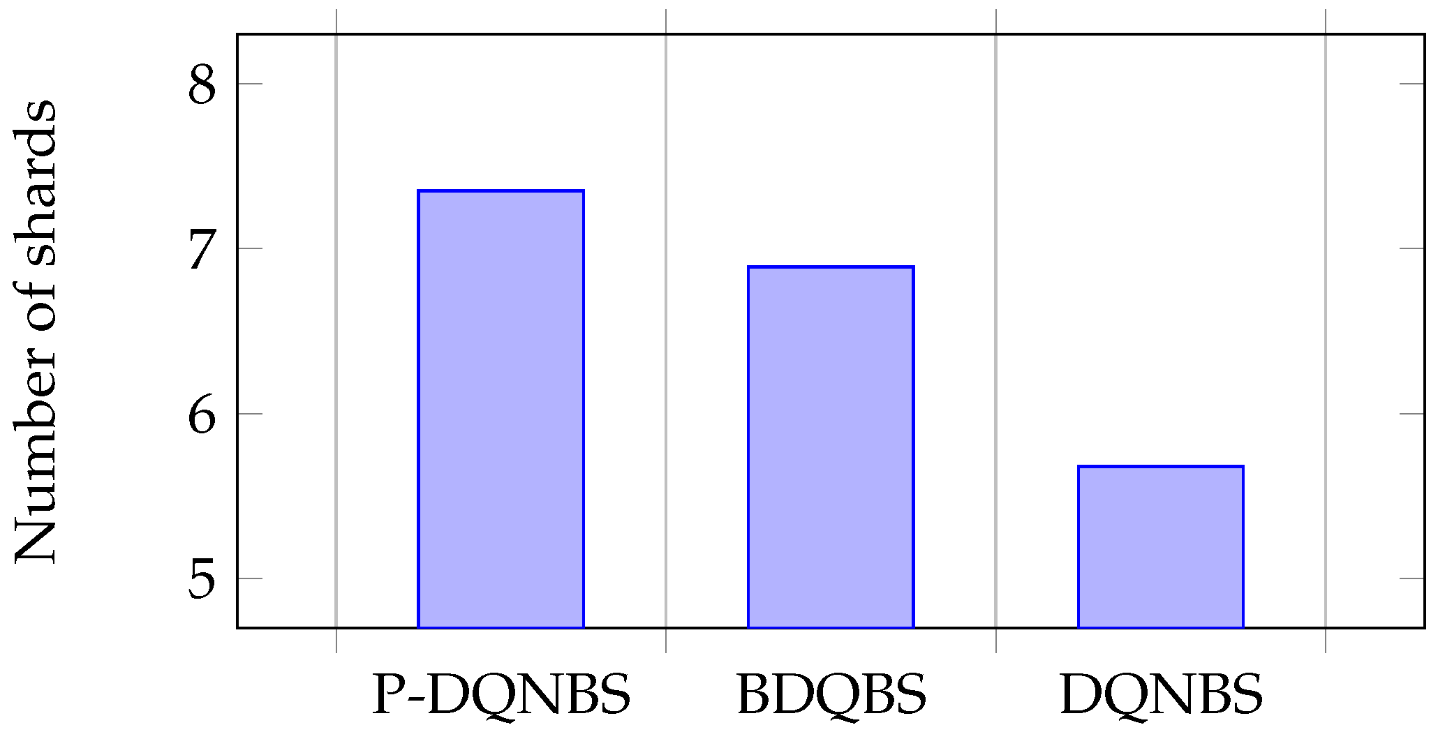
Sub-action K represents the number of shards. In Figure 7, the average value of sub-action K in the BDQBS is 21% higher than in the DQNBS, indicating that BDQBS can shard blockchain nodes into more shards and more transactions can be process in parallel within the shards. The average sub-actions K of the P-DQNBS are 29% and 7% higher than the DQNBS algorithm and BDQBS, respectively. Subaction B represents block size. In Figure 8, the average number of subactions B in the BDQBS is about 5% higher than in the DQNBS, which indicates that the BDQBS handles more transactions than the DQNBS. The average number of subactions B in P-DQNBS is approximately 8% higher than in BDQBS and 12% higher than in DQNBS, indicating that P-DQNBS can enable the blockchain to handle more transactions. The subaction T represent the block generation time. In Figure 9, the average number of subactions T of BDQBS is 7% smaller than that of DQNBS, indicating that using the BDQBS to process data is faster. The average number of subactions T in P-DQNBS is 7% and 13% less than in BDQBS and DQNBS, respectively, which indicates that P-DQNBS can process transactions in the shortest time and has the fastest processing speed. In summary, the BDQBS can improve the throughput of the blockchain compared to the DQNBS. The use of P-DQNBS can improve the performance of blockchain systems the best.

The average execution times per step of the DQNBS, BDQBS and P-DQNBS are $0.27$ s, $0.31$ s and $0.35$ s, respectively. Since the execution times of the algorithms are very short, we output the execution times of twenty consecutive steps and calculate the average value to obtain the average execution time of each step of the algorithm.

5.2.2. Impact of Malicious Node Ratio

A malicious node rejects an honest block in the consensus process or creates a malicious block. Figure 10 shows the TPS under various malicious node ratios. When all nodes in the network are honest, the TPS of P-DQNBS is $1.12$ and $1.17$ times higher than BDQBS and DQNBS, respectively. As malicious nodes emerge, the performance of all algorithms drops, because $K_t$ has to decrease to satisfy constraint C1 and C2 for increased $P_t$, and the number of transactions processed is concurrently reduced. We also observe that P-DQNBS is more robust to malicious nodes since it achieves higher TPS in all simulations.

5.2.3. Average Latency Comparison

To improve the throughput, an obvious approach is to increase the number of shards and the block size while maintaining a small block interval. However, arbitrarily large $K_t$ and $B_t$ values result in longer consensus time $T_{con}^{K_t}$, and together with a small $T_t$, will make constraint C1 and C2 easily violated. It can be shown in Figure 11 that all policies find feasible actions which keep the transaction latency under the threshold, but P-DQNBS learns the best policy with the highest throughput.

5.2.4. Throughput under Different Average Transaction Sizes

Figure 12 shows the throughput using different algorithms under different average transaction sizes. It can be seen that with the increase in transaction size, throughput significantly decreases because of the decreasing number of block packaged transactions. However, the P-DQNBS outperforms the BDQBS and DQNBS in any scale of transactions. When the average transaction size is 100MB, the throughput using the P-DQNBS algorithm is approximately 1.11 and 1.14 times that of the BDQBS and DQNBS. When the average transaction size reaches the maximum value of 500MB, the throughput using the P-DQNBS is approximately 60% and 89% higher than the BDQBS and DQNBS. This indicates that the P-DQNBS can provide better action for blockchains compared to BDQBS and DQNBS when processing transactions of any scale, resulting in an improvement in blockchain performance.

6. Conclusions and Future Work

According to the experimental analysis of P-DQNBS, BDQBS and DQNSB in Section 5.2, the throughput of the three algorithms is obtained in the blockchain simulation environment, and the average action of the three algorithms is compared and analyzed. The experimental comparison shows that the performance of the P-DQNBS is better than that of the BDQBS and the DQNSB. The average TPS of P-DQNBS is $28\%$ and $11\%$ higher than DQNBS and BDQ, respectively. When all nodes in the network are honest, the TPS of P-DQNBS is $1.12$ and $1.17$ times higher than BDQBS and DQNBS, respectively. When the average transaction size reaches the maximum value of 500 MB, the throughput using the P-DQNBS is approximately 60% and 89% higher than the BDQBS and DQNBS. Under a stochastic environment, the throughput of the three algorithms is compared, and the experimental results show that the P-DQNBS can provide the best strategy for the blockchain system and obtain the highest throughput under the condition of satisfying security. In addition, the average latency of the three algorithms is compared, and the experimental results show that the P-DQNBS algorithm has the smallest delay, indicating that the P-DQNBS algorithm can process transactions faster, so that the blockchain can achieve the highest throughput. Finally, the performance of the three algorithms is compared in terms of different average transactions, and the experimental results show that the P-DQNBS can provide the most accurate action strategies for the blockchain and make the blockchain’s performance the best.

We proposed the BDQBS and the P-DQNBS as the optimal blockchain sharding policy. Compared with DQNBS and other algorithms, P-DQNBS does not need to discretize the continuous actions and thereby provides a higher-quality sharding policy for the OBCS problem. This topic mainly studies the research on blockchain performance optimization method based on sharding technology. Traditional blockchain sharding usually takes a static approach, which is not in line with a dynamic blockchain environment. Therefore, DRL is applied to the blockchain sharding problem to provide dynamic sharding decisions for the dynamic blockchain system, so as to improve the performance of the blockchain while establishing the blockchain sharding process as an MDP. The most common DRL algorithm used in the blockchain environment is the DQN, which solves the problem of state space explosion but does not solve the problem of action space explosion. This leads to difficulty in neural network training.

In view of the above problems, we used the BDQ and P-DQN in the blockchain sharding problem and proposed the BDQBS and P-DQNBS. The BDQBS algorithm solves the problem of action space explosion and provides a better action strategy for the blockchain system, thereby improving the blockchain’s performance. The action space of the blockchain sharding problem is a discrete–continuous hybrid action space, and the BDQBS algorithm mainly solves the problem of discrete action space, so the continuous action is discretized to obtain the discrete action space. However, this approach ignores more precise action, so we applied the P-DQN to solve the problem, and proposed the P-DQNBS algorithm. The P-DQNBS algorithm provides a more accurate sharding strategy for the blockchain system, which further improves the performance of the blockchain.

This project takes optimizing the blockchain performance based on sharding technology as the main goal, and designs a blockchain sharding selection strategy based on DRL. Although certain results have been achieved, due to limitations on time and experimental conditions, there are still some shortcomings which need more in-depth research and improvement in the later stage. The experimental algorithm verifies the implementation based on the built blockchain shard simulation environment. However, the real blockchain system will inevitably have more dynamic changes. For example, the transmission rate between nodes and the computing power of nodes must be different. Due to the limited experimental conditions, it is necessary to perform algorithm verification in the real blockchain environment in the future. We use network sharding to partition blockchain nodes, and there is a problem of transaction cross-sharding when using network sharding, which leads to the problem of double spending. So, in the future, it will be necessary to supplement and improve the research on blockchain transaction sharding and state sharding. Blockchain transaction sharding and state sharding are research trends in improving blockchain throughput in the future.

References

- Guo, S.; Hu, X.; Guo, S.; Qiu, X.; Qi, F. Blockchain meets edge computing: A distributed and trusted authentication system. IEEE Trans. Ind. Inform. 2019, 16, 1972–1983. [Google Scholar] [CrossRef]
- Wan, J.; Li, J.; Imran, M.; Li, D.; Fazal-e-Amin. A blockchain-based solution for enhancing security and privacy in smart factory. IEEE Trans. Ind. Inform. 2019, 15, 3652–3660. [Google Scholar] [CrossRef]
- Yun, J.; Goh, Y.; Chung, J.M.; Kim, O.; Shin, S.; Choi, J.; Kim, Y. MMOG user participation based decentralized consensus scheme and proof of participation analysis on the bryllite blockchain system. KSII Trans. Internet Inf. Syst. (TIIS) 2019, 13, 4093–4107. [Google Scholar]
- Zheng, Z.; Xie, S.; Dai, H.; Chen, X.; Wang, H. An overview of blockchain technology: Architecture, consensus, and future trends. In Proceedings of the 2017 IEEE International Congress on Big Data (BigData Congress), Honolulu, HI, USA, 25–30 June 2017; pp. 557–564. [Google Scholar]
- Yao, H.; Mai, T.; Wang, J.; Ji, Z.; Jiang, C.; Qian, Y. Resource trading in blockchain-based industrial Internet of Things. IEEE Trans. Ind. Inform. 2019, 15, 3602–3609. [Google Scholar] [CrossRef]
- Wood, E. A secure decentralised generalised transaction ledger, Ethereum Proj. Yellow Pap. 2014, 151, 1–32. [Google Scholar]
- Androulaki, E.; Barger, A.; Bortnikov, V.; Cachin, C.; Christidis, K.; De Caro, A.; Enyeart, D.; Ferris, C.; Laventman, G.; Manevich, Y.; et al. Hyperledger fabric: A distributed operating system for permissioned blockchains. In Proceedings of the Thirteenth EuroSys Conference, Porto, Portugal, 23–26 April 2018; pp. 1–15. [Google Scholar]
- Nguyen, L.N.; Nguyen, T.D.; Dinh, T.N.; Thai, M.T. Optchain: Optimal transactions placement for scalable blockchain sharding. In Proceedings of the 2019 IEEE 39th International Conference on Distributed Computing Systems (ICDCS), Dallas, TX, USA, 7–10 July 2019; pp. 525–535. [Google Scholar]
- Luu, L.; Narayanan, V.; Zheng, C.; Baweja, K.; Gilbert, S.; Saxena, P. A secure sharding protocol for open blockchains. In Proceedings of the 2016 ACM SIGSAC Conference on Computer and Communications Security, Vienna, Austria, 24–28 October 2016; pp. 17–30. [Google Scholar]
- Kokoris-Kogias, E.; Jovanovic, P.; Gasser, L.; Gailly, N.; Syta, E.; Ford, B. OmniLedger: A Secure, Scale-Out, Decentralized Ledger via Sharding. In Proceedings of the IEEE Symposium on Security and Privacy, Francisco, CA, USA, 20–24 May 2018; pp. 583–598. [Google Scholar]
- The Zilliqa Team. The Zilliqa Technical Whitepaper. 10 August 2017. pp. 1–14. Available online: https://docs.zilliqa.com/whitepaper.pdf (accessed on 4 December 2023).
- Zamani, M.; Movahedi, M.; Raykova, M. RapidChain: Scaling Blockchain via Full Sharding. In Proceedings of the the 2018 ACM SIGSAC Conference, Toronto, ON, Canada, 15–19 October 2018. [Google Scholar]
- Yun, J.; Goh, Y.; Chung, J.M. DQN-based optimization framework for secure sharded blockchain systems. IEEE Internet Things J. 2020, 8, 708–722. [Google Scholar] [CrossRef]
- Zhang, J.; Hong, Z.; Qiu, X.; Zhan, Y.; Guo, S.; Chen, W. Skychain: A deep reinforcement learning-empowered dynamic blockchain sharding system. In Proceedings of the 49th International Conference on Parallel Processing-ICPP, Edmonton, AB, Canada, 17–20 August 2020; pp. 1–11. [Google Scholar]
- Gervais, A.; Karame, G.O.; Wüst, K.; Glykantzis, V.; Ritzdorf, H.; Capkun, S. On the security and performance of proof of work blockchains. In Proceedings of the 2016 ACM SIGSAC Conference on Computer and Communications Security, Vienna, Austria, 24–28 October 2016; pp. 3–16. [Google Scholar]
- Castro, M.; Liskov, B. Practical byzantine fault tolerance and proactive recovery. ACM Trans. Comput. Syst. 2002, 20, 398–461. [Google Scholar] [CrossRef]
- Sukhwani, H.; Martínez, J.M.; Chang, X.; Trivedi, K.S.; Rindos, A. Performance modeling of PBFT consensus process for permissioned blockchain network (hyperledger fabric). In Proceedings of the 2017 IEEE 36th Symposium on Reliable Distributed Systems (SRDS), Hong Kong, China, 26–29 September 2017; pp. 253–255. [Google Scholar]
- Syta, E.; Jovanovic, P.; Kogias, E.K.; Gailly, N.; Ford, B. Scalable Bias-Resistant Distributed Randomness. In Proceedings of the 2017 IEEE Symposium on Security and Privacy (SP), San Jose, CA, USA, 22–26 May 2017; pp. 444–460. [Google Scholar]
- Yao, B.; Wan, J.; Shan, J.; Li, L.; Ma, Z.; Liu, C. Optimal Sharding for Dynamic Throughput Optimization in Blockchain Systems with Deep Reinforcement Learning. In Proceedings of the 2023 IEEE Conference on Systems, Man, and Cybernetics, Honolulu, HI, USA, 1–4 October 2023; pp. 1–5. [Google Scholar]
- Król, M.; Ascigil, O.; Rene, S.; Sonnino, A.; Al-Bassam, M.; Rivière, E. Shard scheduler: Object placement and migration in sharded account-based blockchains. In Proceedings of the 3rd ACM Conference on Advances in Financial Technologies, Arlington, VA, USA, 26–28 September 2021; pp. 43–56. [Google Scholar]
- Xiong, J.; Wang, Q.; Yang, Z.; Sun, P.; Han, L.; Zheng, Y.; Fu, H.; Zhang, T.; Liu, J.; Liu, H. Parametrized deep q-networks learning: Reinforcement learning with discrete-continuous hybrid action space. arXiv 2018, arXiv:1810.06394. [Google Scholar]
- Sutton, R.; Barto, A. Reinforcement Learning: An Introduction; The MIT Press: Cambridge, MA, USA, 1998. [Google Scholar]
- Paul, L.T.; James, H.J.; David, S.; Tom, E.; Yuval, T.; Otto, H.N.M.; Pieter, W.D.; Alexander, P. Continuous control with deep reinforcement learning. arXiv 2018, arXiv:1509.02971. [Google Scholar]
- Mnih, V.; Kavukcuoglu, K.; Silver, D.; Rusu, A.A.; Veness, J.; Bellemare, M.G.; Graves, A.; Riedmiller, M.; Fidjeland, A.K.; Ostrovski, G.; et al. Human-level control through deep reinforcement learning. Nature 2015, 518, 529–533. [Google Scholar] [CrossRef] [PubMed]
- Paszke, A.; Gross, S.; Massa, F.; Lerer, A.; Bradbury, J.; Chanan, G.; Killeen, T.; Lin, Z.; Gimelshein, N.; Antiga, L.; et al. Pytorch: An imperative style, high-performance deep learning library. Adv. Neural Inf. Process. Syst. 2019, 32, 8026–8037. [Google Scholar]