Abstract
Pressure sensors embodied in very tiny packages are deployed in a wide range of advanced applications. Examples of applications range from industrial to altitude location services. They are also becoming increasingly pervasive in many other application fields, ranging from industrial to military to consumer. However, the inexpensive manufacturing technology of these sensors is strongly affected by environmental stresses, which ultimately affect their measurement accuracy in the form of variations in gain, hysteresis, and nonlinear responses. Thermal stresses are the main source of sensor behavior deviation. They are particularly insidious because even a few minutes of high temperature exposure can cause measurement drift for many days in the sensor responses. Therefore, conventional calibration techniques are challenged in their adequacy to achieve high accuracy and over the entire deployment life of the sensor. To manage this, several costly and time-consuming calibration procedures have to be performed. Machine learning (ML) techniques are known, supported by the universal approximation theorem, to provide effective data-driven solutions to the above problems. In this context, this paper addresses two case studies, corresponding to post-soldering thermal stresses and exposure to moderately high temperatures, for which two separate datasets have been built and 53 different tiny ML models (collected into a zoo) have been devised and compared. The ML zoo has been constructed with models such as artificial neural networks (ANN), random forest (RFR), and support vector regressors (SVR), able to predict the error introduced by the thermal drift and to compensate for the drift of the measurements. The models in the zoo also satisfy the memory, computational, and accuracy constraints associated with their deployment on resource-constrained embedded devices to be integrated at the edge. Quantitative results achieved by the zoo are reported and discussed, as well as their deployability on tiny micro-controllers. These results reveal the suitability of a tiny ML zoo for the long-term compensation of MEMS pressure sensors affected by drift in their measurements.
1. Introduction
In the current era of IoT, Industry 4.0, localization services, and humanoid robotics, pressure sensors are essential enablers. They are deployed in a wide range of compelling applications, including altitude localizers, industrial, biomedical, automotive, robotics, wearable, home, AV/VR, GPS, drones, e-cigarettes, gas metering, and many more appliances. The associated market size is currently valued at USD 18.73 billion, and it is expected to grow at a compound annual growth rate (CAGR) of 4.3% between 2023 and 2030, according to [1].
State of the art pressure sensors are based on tiny, cheap, and long-lasting micro-electro-mechanical systems (MEMS) technology [2], which leverages the mechanical response of a mobile element set to produce an accurate electrical signal through an analog and digital signal processing pipeline. More specifically, MEMS pressure sensors feature a silicon membrane, which, when pressure is applied, deflects. This induces an imbalance in the Wheatstone bridge piezoresistance [3]. Next, the output signal is used to infer the pressure measurement.
Temperature sensors, usually, are super-integrated with pressure sensors in the same sensor package. Unfortunately it is rare that this measure is available at the output of the sensor’s interfaces to the external world. Pressure and temperature measurements are natively analog, processed as such, and then A/D converted. This allows them to be communicated to an external microprocessor (MPU) or controller unit (MCU) for further processing. In many applications, MEMS-based pressure sensors are required to provide accurate, reliable, and high-confidence measurements. This is particularly true for altitude location-based services in which pressure is used to infer the sensor’s altitude to locate the sensor’s owner in a building. For this purpose, they are factory-calibrated once and immediately after they are signed off. During their deployment, however, pressure sensors experience a broad range of stress conditions, which ultimately affect their measurements in the form of variations in gain, hysteresis, and sensitivity [4,5].
Drops in supply voltage, exposure to high temperatures for short or long periods, different operating temperatures, and exposure to soldering are the factors causing the sensor to experience drift from its nominal behavior. For example, the grains created by metal nucleation during the deposition process inside the sensor impact the metal alloy’s stabilization by deforming the lattice. In turn, as shown in Figure 1, this creates non-reversible thermoplastic hysteresis effects on the pressure measurements for a quite long time. These events are responsible for consistently degrading the accuracy of the sensor readings.
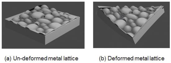
Figure 1.
(a) The sensor’s metal lattice before thermal stresses; (b) the sensor’s metal lattice deformed by the thermal stresses. Metal grains are displaced with respect to the original placement, causing hysteresis in the measurements.
Therefore, drift compensation is needed to mitigate these systematic and time-varying errors. Errors could be either random or systematic. The former are not addressed in this paper. Instead, this work addresses the compensation of systematic errors, and, more specifically, the errors caused by two factors: the inevitable soldering of the sensor on a motherboard during, for example, smartphone manufacturing, and the long-term exposure of the sensor to moderately high temperatures during its deployment in the field and in a smartphone.
It is evident that calibration should not be performed only once during manufacturing. Instead, it should be continuously performed during the entire deployment life of the pressure sensor. However, this could be prohibitive, costly, complex, and time-consuming to realize in practice. Indeed, the most common, fast to achieve during manufacturing, and low-complexity technique to implement calibration is called One Point Calibration (OPC). It takes a measurement from the sensor at 25 °C and compares it with the measurement from a reference, highly accurate (and very costly) barometer. Then, the calibration offset is computed by subtracting the sensor’s reading from the reference. During successive (in time) measurements, the offset will be added to the sensor readings in order to compute the calibrated, error-free, value. OPC computes a non-time-varying offset in a precise environmental condition and in one instant of time, which cannot be scaled or generalized to other conditions that are encountered by the sensor during its lifetime. A method like OPC has a major drawback: it requires frequent offset re-computation and the availability of a reference barometer. Indeed, OPC assumes the calibration error to be constant or linearly varying over time, which is usually not representative of the real case. A more efficient alternative to OPC is based on machine learning (ML) and deep learning (DL) techniques. The training procedures of ML/DL models take advantage of the reference barometer to generate training data. Once these models are trained and deployed, the pressure sensor will be able to predict nonlinear and time-varying compensations for pressure measurements via the ML/DL inferences.
Hence, the limitations of the OPC procedure have motivated the investigation of various calibration methods that rely on DL and ML workloads. Indeed, the establishment of DL and ML has been transformative across a broad variety of domains [6], including, for instance, image classification [7] and seasonal and trend time series forecasting [8,9]. Their success is underpinned by the universal approximation theorems [10], which highlight the ability of artificial neural networks (ANN) to approximate continuous functions to any degree of accuracy [11], making ANNs one of the most powerful approaches to achieve function approximation. However, they should be deployable in the resource-constrained assets of a sensor and be useful to everyone in everyday life at a very low cost.
In this context, this paper addresses the challenge of defining several tiny ML and DL models deployable for sensor calibration as alternatives to the OPC methodology. Moreover, these models shall be deployable in MEMS pressure sensors with built-in ML computing capabilities, available in a single package. The paper is organized as follows. Section 2 introduces the need for accurate pressure sensors in real-life applications; Section 3 introduces two case studies that define the acquisition process of the corresponding datasets; Section 4 describes the research question that this paper addresses through ML/DL solutions. These solutions are intended to fulfill the corresponding requirements. Section 5 reviews related works that have either anticipated answers to the research question or provided useful insights; Section 6 details the datasets that shape the case studies defined in Section 3; Section 7 describes the ML/DL models that address the research question and are trained using the datasets described in Section 6; Section 8 reports the quantitative results achieved by the proposed models in Section 7; Section 9 discusses the results listed in Section 8 and provides a deployability analysis on a tiny micro-controller of the selected DL/ML models; Section 10 concludes this work; and Section 11 introduces perspectives for future work.
2. Pressure Sensor for Vertical Position Localization
Pressure sensors are instrumental in estimating smartphones’ vertical positions in many application scenarios. The inverse relationship between air pressure variations with respect to the altitude allows one to localize it vertically, as described by [12]. These sensors, which lack any horizontal estimation capability, offer unique advantages (e.g., cost, simplicity, small form factor, μW power consumption) compared to Global Positioning Systems (GPS). GPS devices, which are commonly used in providing vertical location information too, are challenged in their accuracy, as highlighted in [13].
One life-saving application is floor level localization in buildings for people rescue under emergencies (e.g., fires, earthquakes, etc.). Current response systems often struggle to accurately locate individuals on a specific floor in a building based solely on voice indications provided during an emergency call.
Other than emergency situations, indoor navigation systems benefit significantly from accurate vertical position estimation, enabling seamless movement through expansive and intricate indoor spaces. Therefore, with such an approach, the traditional GPS limitations in indoor settings are overcome, opening up possibilities for navigation, for example, through multi-level shopping malls, parking lots, busy airports, complex subway stations, and dynamic fairs. The implications extend to enhancing the user experience by facilitating efficient and accurate movement and aiding in locating specific points of interest, such as booths at multi-floor conferences or trade fair venues. Moreover, the application of pressure sensors in fitness tracking adds a new dimension to activity monitoring. By measuring the number of floors climbed, users can gain valuable insights into the intensity and elevation of their physical activity. The work presented in [14] offers more insights on the topic of indoor positioning.
3. Case Studies
If a sensor measurement is not calibrated with respect to a ground truth value, an un-calibration event is said to have occurred. At the industry level, the sensors are usually calibrated in a half second during their manufacturing. However, when deployed in real-world applications, various real-life conditions can cause anomalies within the sensor. Anomalies can often take a variety of shapes, such as non-reversible deformations of the composing materials. They typically cause hysteresis measurements and long-term drifts affected by a variety of responses, including linear, exponential, logarithmic, or atypical drifts [15,16].
This work is focused on piezoresistive pressure sensors that are affected by hysteresis phenomena due to thermal stresses, which cause time-varying drifts that affect sensor measurements for several days after their occurrence. The inevitable soldering process of the sensor in the application motherboard significantly impacts the measurements of the sensors [15], as considered in this paper. A real-life scenario such as prolonged exposure to moderately high temperatures, similar to [16], is also considered within the scope of this work.
In summary, an exemplary pressure sensor, widely used by the industry, and two significant case studies are considered.
3.1. The LPS22HH Pressure Sensor
As a realistic, widely deployed and adopted industry example, the pressure sensor named LPS22HH is considered in this study. It is a tiny piezoresistive absolute pressure sensor that operates as a digital (at the output) and very cheap barometer [17]. The device is composed of two key elements: a sensing component and an IC interface. The latter communicates the measurements to an external MCU or MPU, through I2C, MIPI, I3CSM, or SPI interfaces. The former is designed to sense the absolute pressure and is built with a dedicated 130 silicon manufacturing process, to implement a suspended membrane.
The sensor is enclosed in a full-molded holed LGA (HLGA) package. It is designed to operate reliably within a specified operative temperature range of −40 °C to +85 °C. The sensor package features perforations to enable external pressure to reach sensing element. Additionally, the sensor has an absolute maximum ratings temperature range, which spans from −40 °C to +125 °C. It is underlined that any exposure to temperatures beyond these limits can result in permanent damage to the device, affecting the reliability of the measurements.
3.2. Case Study A: Soldering Drift
Reflow soldering is a technique used to create permanent solder joints between sensor devices and a printed circuit board (PCB) using solder paste. This process involves standard controlled heating, which can be achieved through different techniques, such as passing the assembly through a reflow oven, using an infrared lamp, or, less conventionally, soldering individual joints with a hot air pencil. The primary objective of the reflow process is to raise the solder paste to its eutectic temperature, causing the solder alloy to change from a solid to a liquid or molten state. At this specific temperature range, the molten solder exhibits excellent adhesion properties [18]. It is important to note that the sensor device is turned off during the reflow soldering process; therefore, no measurements can be acquired.
The temperature profile in a reflow oven is tailored to suit the characteristics of a particular PCB assembly, taking into account factors such as the number of PCB layers, the quantity and size of components, and many others. According to the IPC/JEDEC J-STD-020C Standard [18], the temperature can reach from 183 °C to 217 °C for 60 to 150 s and 260 °C for 10 to 40 s. This standard temperature profile ensures that the solder reflows onto adjoining surfaces without exceeding the temperature tolerance of the electrical components, thereby preventing damage.
Figure 2 represents the temperature with respect to time according to the IPC/JEDEC J-STD-020C Standard [18]. It represents the different stages during the soldering process. Each of these stages has a specific thermal profile designed to achieve optimal soldering results while safeguarding the components from overheating.
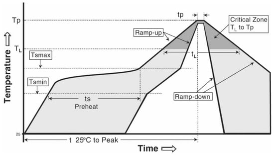
Figure 2.
Temperature profile phases during reflow soldering according to the IPC/JEDEC J-STD-020C Standard [18].
According to these premises, case study A investigates simulations of reflow soldering to study the post-soldering drift, similarly to the use case in [15].
3.3. Case Study B: Normal Usage with Long Exposure to (Moderately) High Temperatures
A non-standard test has been defined in this work. Associated studies were conducted to assess the sensor’s performance after a prolonged period of thermal stress. The study was concerned with the sensor’s ability to function as expected outside the recommended operating conditions—in particular, whether it would experience temperature fluctuations between 85 °C and 125 °C, and then return to the nominal operating range. Would the device then continue to operate correctly? Unlike the JEDEC soldering procedure, there is no standard procedure, to the authors’ knowledge, for such a test [16]; therefore, this work devised one. Taking into account the sensor’s nominal characteristics and considering the average time to stress it during normal usage, the simulation of this case study was performed by exposing the sensor to a thermal budget of 100 °C for two hours.
4. Research Question and Associated Requirements
The question that this study sought to answer quantitatively was the following: How tiny can a machine learning model be designed to provide accurate drift compensation for the use cases defined in Section 3.2 and Section 3.3? To be considered a valid answer to this question, a model should fulfill the following requirements.
- The candidate model’s footprint should not exceed 2 MB in order to fit into the embedded memory of a resource-constrained target device, such as a micro-controller or embedded processor, which are typically employed in edge computing architectures.
- The number of parameters of the model should be lower than a half to one million.
- The ratio of training samples to model parameters should not be lower than ten.
- The model should be deployable in a low-power sensor’s built-in ML assets.
- The model has to be accurate. There is no acceptable argument that support the adoption of any processing solution that achieves a signal-to-noise ratio (S/N) below the one that features the sensor data.
- Precisely, the accuracy of the compensation should be within ±50 Pa, as defined by [17]. Since pressure data are coded into 24 bits, the S/N is required to be 144 dB. Hence, any solution should achieve an S/N above this value.
Some of the requirements defined above are essential to achieve a tiny ML solution. As a consequence, Table 1 highlights the three most salient requirements that are relevant to this work.

Table 1.
Essential requirements for this work.
5. Related Works
Many ML and DL approaches have been proposed in the literature for the calibration of pressure sensors affected by aging, environmental variations, and thermal drift. Most of the related works, however, consider only static calibration; therefore, they do not take into account the temporal duration of the un-calibration caused by the sensor’s exposure to high temperatures, even if for a limited amount of time. Such exposure could generate effects that last for several days, as observed in the post-soldering use case.
5.1. Static Calibration
The compensation of thermal drift in a silicon piezoresistive pressure sensor was proposed in [4] by transferring an Extreme Learning Machine (ELM) trained on a personal computer (PC) to an external MCU. The ELM improved the accuracy temperature coefficient in the nominal −40–85 °C range from 2.57% FS to 0.13% FS and, due to its shorter training time, was suitable for batch compensation.
A similar approach was embraced by [19], using an ELM that had as inputs the output of the sensor and the non-target parameters, i.e., temperature and voltage fluctuations. It mapped them to the true pressure value. In the experiments, the model achieved a mean squared error (MSE) of 0.338 with a training duration of 1.35 s. Additionally, the proposed method was compared with the backpropagated neural network (NN) and a support vector machine (SVM). The proposed ELM achieved better accuracy and stability and had a shorter training time and lower application costs. The ELM was deployed on a commodity PC, which was costly compared to the low-memory budget requirements set by this work.
A new method for the calibration of micro-mechanical capacitive pressure sensors (CPS) using an electrical-only and machine learning approach was detailed in [20]. The proposed approach relied on a two-stage algorithm. The training stage established correlation curves and coefficients between electrical and physical data for a limited set of devices. In the testing stage, these correlations were used to reconstruct physical points for the calibration of new devices. It achieved average absolute accuracy of 1.74 hPa within the 600–1100 hPa pressure range. The electrical-only calibration method reduced the test time by more than 85% against traditional methods, offering a rapid and cost-effective solution for pressure sensor calibration. The focus on capacitive MEMS pressure sensors differs from the piezoresistive sensor considered in this study.
An ANN-based scheme for the calibration of CPS sensors in harsh environments (extreme ambient temperature, pressure, humidity, etc.) was proposed in [21]. By employing a backpropagation ML algorithm with a variable learning rate and incorporating random samples in the training process, a CPS calibration model was developed. Both linear and three types of nonlinear influences of temperature on the sensor characteristics across a temperature range from −50 to 200 °C were evaluated through computer-simulated experiments. The NN model’s maximum full-scale error in pressure estimation fell within ±1.0% for the linear form and within ±1.5% for the three nonlinear influences.
An alternative approach involving the usage of a wavelet neural network (WNN) was adopted in [22] for temperature compensation in silicon piezoresistive pressure sensors. The model took as input temperature and pressure readings from the sensor and produced as output the true pressure value. Furthermore, the solution was compared with standard BP neural networks. The results revealed that the WNN achieved a RMSE, while the latter had a RMSE. Ref. [23] proposed a polynomial-based adaptive digital temperature compensation method for automotive piezoresistive pressure sensors. The compensation technique effectively addressed the nonlinear temperature dependency of the pressure sensor by leveraging opposite characteristics as a function of temperature. Implementing the compensation polynomial in a digital system, the approach also incorporated a scaling technique to enhance the accuracy while adopting a resource-sharing technique to minimize the controller area and power consumption. Additionally, the shared structure approach integrated a high-resolution sigma-delta analog-to-digital converter (ADC) for improved accuracy across a wide temperature range (−40 °C to 150 °C). The measured temperature compensation accuracy was reported to be within ±0.068% with a full scale, and the entire technique was integrated into an automotive pressure sensor signal conditioning chip using a 180 nm complementary metal–oxide–semiconductor (CMOS) process.
A CMOS analog ASIC of a feedforward NN (FFNN), based on both a conventional neuron model and an inverse delayed function model of the neuron, was designed in [24] for the temperature drift compensation of high-resolution piezoresistive MEMS pressure sensors. The inverse delayed function model yielded a mean square error in the order of for the neural network, significantly outperforming the conventional neuron model, with a mean square error in the order of for the same ANN architecture. This resulted in a remarkable reduction in error, from 9% for an uncompensated sensor to only 0.1% for a compensated sensor, within the temperature range of 0–70 °C, using the delayed model of the neuron. In contrast, compensation with a conventional neuron-based ANN reduced the error to 1%.
The escalating legal pressures from regulatory authorities have resulted in heightened demands for resilient pressure sensors in vehicles. Consequently, ref. [25] proposed a cost-effective smart piezoresistive pressure sensor that integrated signal conditioning, analog/digital signal processing, and communication circuitry directly into the sensor element within a single compact housing system. The smart pressure sensor offered enhanced reliability and accuracy through built-in features such as temperature compensation, filtering, and self-calibration. The latter was obtained through a two-layer feedforward ANN architecture trained with Levenberg–Marquardt backpropagation and deployed on an external MCU. The ANN received as input the output pressure indicated by the signal conditioner and it output the true pressure value. After testing the sensor calibration system, the accuracy achieved was FS, as opposed to FS indicated in the datasheet of the bare sensor.
5.2. Dealing with Small Datasets
One of the main issues to tackle when developing an NN model for sensor compensation is the small size of the calibrated data. To address this issue, ref. [26] leveraged data augmentation by learning the calibration process of pressure sensors through the proposed Aquila optimized mixed polynomial kernel ELM (AO-MPKELM) algorithm. Results showed strong consistency between real and generated data, with a maximum voltage deviation of 0.71 mV. Compensating through bilinear interpolation, measurement errors were reduced by 78.95% with full-scale accuracy of 0.03%.
Standard procedures for pressure sensor calibration consist of subjecting the recently manufactured sensors to several controlled temperature and pressure set points to fit a polynomial mapping between the sensor’s predicted value and true pressure. The large number of pressure and temperature set points required by this approach makes it costly, time-consuming, and impractical for industrial deployment. An alternative solution is adopting an ML model to predict the calibration polynomial’s parameter using fewer calibration data, learning from past calibration sessions [27]. The proposed solution considers a novel polynomial hyper-network coupled with Fourier features and a weighted loss. Extensive evaluations show that such an approach saves two thirds of the calibration time and cost.
As the use of ANNs for calibration processes has been limited due to issues like lower training speeds, local minima, and overfitting due to few data available, an SVR model was adopted in [28] to compensate for the pressure sensor’s nonlinearity influenced by temperature and voltage fluctuations. The proposed model established a mapping relationship between the actual voltage output characteristics and pressure sensor nonlinearity, reducing the error from 22.2% to 0.64% in the proposed experiments. The SVM’s calibration model, applied to the CYJ-101 Pressure Sensor, demonstrated improved accuracy and stability, offering a viable solution for sensors affected by temperature and voltage fluctuations. The self-adaptive adjustment of parameters further enhanced the model’s effectiveness.
A similar approach was adopted by [29], which modeled the complex hysteresis of a diffused silicon pressure sensor through a Preisach model obtained by regression analysis from experimental data. Considering the limited amount of samples, the SVR approach led to better results with respect to BP neural networks, as the latter overfitted. This corroborated the superiority in terms of accuracy of SVM, in comparison with NNs, when operating in a few-samples regime.
5.3. Evolutionary Algorithm Approaches
An alternative approach to avoid overfitting and local optima due to the small amount of available calibrated data consists of the use of evolutionary algorithms. Ref. [30] adopted three different types of swarm optimization algorithms in combination with ML models for the temperature compensation of three different ranges of sensors. It achieved a zero-drift coefficient of /°C and a sensitivity temperature coefficient of /°C. In another study, ref. [31] presented adaptive mutation particle swarm optimization optimized support vector regression (AMPSO-SVR) integrated with an improved version of AdaBoost. The RT algorithm was used to calibrate the ambient temperature nonlinearity in a silicon piezoresistive pressure sensor. Results were superior compared to other methods and the AMPSO algorithm successfully avoided local optima in the model parameters.
5.4. Temporal Dependence of Sensor Drift
The aforementioned methods do not address the temporal-dependent aspect of the sensor drift. A candidate solution is to use sequential DL models such as a gated recurrent unit (GRU) and long short-term memory (LSTM). In such a context, ref. [32] proposed a multi-class classifier model based on the combination of an improved LSTM and SVM for drift compensation in gas sensors. The higher classification accuracy, however, was achieved at the price of high model complexity. Similarly, ref. [33] adopted an LSTM for the calibration of air pressure sensors in order to account for the temporal characteristics of the measurement data. The test outcomes on the pressure sensor dataset within the range of [0 kPa, 1100 kPa] and [−30 °C, 30 °C] indicated that, in comparison to other sensor calibration methods, such as BP and radial basis function (RBF) networks, the pressure sensor error was decreased from 1.4 kPa to approximately 0.55 kPa, while the overall calibration speed was not improved. On the other hand, ref. [34] adopted a deep sequential model named Concatenated GRU and Dense Layer with Attention (CGDA) for environmental and time drift compensation in economic gas sensors. The hourly drift sequence was predicted with mean accuracy of over 93% by the model for an entire day.
As an alternative to sequential models, the time dimension as an input to the model has been considered. This is somewhat similar to the approaches proposed by this work. Ref. [35] proposed a real-time self-calibration process based on the Levenberg–Marquardt backpropagation ANN model for pressure estimation in a grasped object using a wearable robotic hand glove. In the experimental setup, a load cell force sensor was used as a reference for the calibrated data obtained during 20 min dynamical loading with 28 repetition cycles. To capture the time dependence of the calibration error, the inputs to the model were the registered voltage and the number of pulses. The method achieved a maximum mean square error of 0.17325 and an R-value over 0.99 for the total response of training, testing, and validation. Unfortunately, the use of a load cell force sensor is not within the scope of this work.
6. Datasets
Datasets for the case studies in Section 3.2 and Section 3.3 were generated in the STMicroelectronics MEMS Sensor Characterization and Measurement Laboratory, by collecting and analyzing several product batches. A collection of recorded pressure and temperature measurements was carefully acquired. They were obtained using the temperature sensor integrated into the LPS22HH [17]. As result of this work, four different datasets were generated: one for Section 3.2 and three for Section 3.3.
6.1. Dataset A for Soldering Drift Case Study
Pressure data were collected from 80 LSP22HH sensors, sampled randomly from several production batches. They underwent the soldering type of thermal stress, compliant with the IPC/JEDEC J-STD-020C Standard [18]. These measurements were collected for 246.5 h after the soldering process was completed, in ambient temperature conditions. The reference barometer measurements were subtracted from the sensor measurements (Psensor − Pref), to derive the accuracy pressure curves plotted in Figure 3.
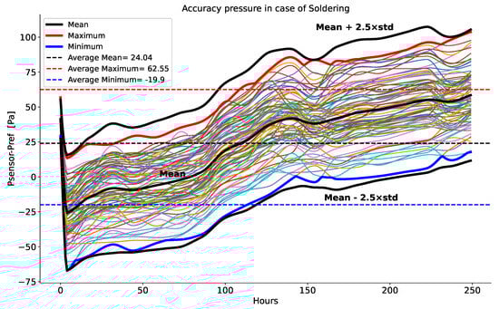
Figure 3.
Post-soldering accuracy pressure curves: reference measurements were subtracted from pressure measurements of 80 devices (Psensor−Pref) for 246.5 h and after the soldering stress was completed. Pressure accuracy curves of different colors represent Psensor−Pref of different sensors. This stress was compliant with the IPC/JEDEC J-STD-020C Standard [18].
Each sensor contributed 250 data, one sample per hour, which formed a curve representing the accuracy of the pressure measurements. Figure 3 graphically displays the 80 curves as well as three key measures:
- The mean—it represents the instantaneous average or central tendency of the pressure accuracy measurements;
- The maximum—this curve illustrates the highest accuracy pressure value recorded by the sensors at each hour;
- The minimum—this curve shows the lowest pressure accuracy value recorded by the sensors at each hour.
Additionally, the standard deviation, denoted as std in Figure 3, was computed to quantify the degree of variation or spread in the pressure accuracy data. The generated curves are within a range that extends the values 2.5 times std below and above the mean pressure accuracy curve. The averages for the maximum, mean, and minimum curves across all 250 samples are represented.
6.2. Dataset B for Normal Usage of Long Exposure to (Moderately) High Temperatures Case Study
To collect data, six LPS22HH sensors, named Devices Under Test (DUT), precisely called DUT1, DUT4, DUT9, DUT12, DUT18, and DUT23, were exposed to prolonged thermal stress of 100 °C for two hours. After this time passed, pressure data were collected over approximately 25 days at ambient temperature.
A seventh DUT (named DUT17) was calibrated and adopted as the reference to compute the accuracy curves (Psensor−Pref). They represented the pressure measurements of the reference subtracted from the pressure measurements of DUTi, with i taking values of 1, 4, 9, 12, 18, and 23, as depicted in Figure 4.
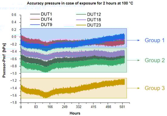
Figure 4.
Accuracy pressure for dataset B: prolonged exposure (2 h) to moderately high temperatures (100 °C). The data acquisition took 596 h (approximately 25 days), after the thermal stress was completed. The data belonged to six DUTs that were classified into three main groups based on the standard deviations of the measures at their outputs, and then augmented in order to compile three different datasets.
Differently from dataset A, the accuracy curves exhibited notable variations in their shapes, influenced by the tolerances inherent to the fabrication process of the DUTs. By observing these variations, the accuracy curves were categorized into three main groups based on their standard deviations relative to the curves of their mean values.
In Figure 4 are represented the original data measurements, where
- DUT4 and DUT9 formed the first group;
- DUT1, DUT12, and DUT18 formed the second group;
- DUT23 formed the third group.
Next, each of them was used for data augmentation to generate 100 curves. Random pressure accuracy curves were produced within a range that spanned 2.5 times the standard deviation both below and above the mean curve of the accuracy pressure.
DUT12, DUT18, and DUT23 deviated from the accuracy specifications reported in the LPS22HH sensor datasheet [17] (cf. REQ2 in Table 1). Due to their poor performance, they should have been discarded by the established product quality verification procedures. Instead, this study devised ML/DL models that aimed to provide corrections to compensate for their performance.
Table 2 provides details regarding the number of measured and generated data samples for both the datasheets for Section 3.2 and Section 3.3.
Table 2.
Measured and generated pressure and temperature data for both datasets A and B.
7. Proposed Machine Learning and Deep Learning Model Zoo
The proposed ML/DL model zoo allowed a performance comparison of 53 different topologies designed to be regressors and to output the error in compensating for the sensor measures under drift. In particular, the models output only the systematic errors following the two scenarios as defined in Section 3. The model zoo included ANNs, random forest regressors (RFR) [36], and support vector regressors (SVR) [37]. The latter used the principles of support vector machines to find the hyperplane that best fit a given set of data points for regression tasks, with the aim of minimizing the error within a certain threshold, and it has proven to be effective in a broad variety of applications [37,38], including time series prediction [39]. On the other hand, RFR is an ensemble learning method that instantiates a multitude of decision trees at training time and outputs the mean prediction of the individual trees during inference. The use of decision trees for regression tasks has been already adopted for a wide range of purposes, such as critical temperature estimation in superconductors [40] and precipitation forecasting [41]. To effectively capture the time-dependent aspects of the datasets under consideration, the ANNs proposed in this work were primarily recurrent-based, complemented by temporal convolution networks (TCNs). TCNs utilize convolutions applied to time series data, enabling them to hierarchically capture and analyze relationships across low, intermediate, and high-level time scales [42]. Among the recurrent-based models employed, basic recurrent neural networks (RNNs) were considered [43]. Moreover long short-term memory (LSTM) networks were utilized [44]. LSTMs are known by their ability to learn long-term dependencies through their inner gating mechanism, which controls the flow of temporal information and mitigates the vanishing gradient problem. Instead, gated recurrent units (GRUs) [45], which also feature gating mechanisms, offer a more streamlined architecture that simplifies the processing while maintaining efficacy, often performing on par with LSTMs in various tasks. In addition, a relatively recent development in this domain was considered. The Lagrange Memory Unit (LMU) [46] represents a significant evolution in RNN design. LMUs incorporate principles from the calculus of variations, offering a sophisticated approach to managing internal yet compact memory states, which enhances the network’s capability to process and remember information over extended time periods.
A more detailed discussion of the design approach and training and testing methodologies is provided in the subsequent Section 7.1.
7.1. Design Approach for the Model Zoo: Topology and Number of Parameters
The approach entailed the design of
- 31 TCN models;
- 15 RNN, including 6 LSTMs, 7 GRUs, and 2 LMUs;
- 6 RFRs;
- a single SVR.
Several configurations of these models were built by combining different numbers and types of layers, such as convolution (Conv), LSTM, GRU, LMU, and dense layers. The ANN models also varied in terms of the activation functions used and the number of filters in each Conv layer. The RFR models differed in terms of the number of estimators and the maximum depth, and 6 combinations were produced.
The exploration was not only limited to different typologies, but it also examined different model footprints, by changing the number of their parameters. These variations were instrumental to investigate their deployability on resource-restricted processors, as per the requirements in Table 1 set in this work.
7.2. Training and Testing Methodology
Following the design of the model zoo, the train and test steps were performed for each dataset independently and for each ML/DL model. Since a single dataset was generated for case A and three datasets for case B, a total of 212 train and test iterations were performed to complete the comparison between the ML/DL models in the zoo.
The training process involved splitting the datasets as follows: 80% for training, 10% for validation, and 10% for testing, as shown in Table 3.
Table 3.
Summary of the data splits and input shapes for the ML/DL model zoo.
The training optimized the mean square error (MSE) loss function through the ADAM [47] optimizer. Parameters such as the input shape, data split, loss function, optimizer, learning rate, batch size, and training epochs are reported in Table 4.
Table 4.
List of training parameters for ANN models.
While the same ML/DL models were trained and tested for both case studies A and B, there was a subtle difference in the shape of their inputs. A more detailed explanation is provided in the two following sub-sections.
7.2.1. Case Study and Dataset A
For Section 3.2, the experimentation was conducted using the dataset of pressure accuracy, described in Section 6.1. The model inputs were time and the accuracy pressure that was measured at one time immediately after the soldering process was concluded. The input tensor was of shape (2,1). Splitting the dataset according to the ratios specified in Table 3 resulted in using 64 DUTs for training, 8 DUTs for validation, and an additional 8 DUTs for testing. Considering that each DUT in the dataset had 250 samples, the number of training samples was equal to 16,000. The different training parameters are reported in Table 4. The learning rate was dynamically scheduled by monitoring the validation loss (MSE) such that, when no improvements were observed for consecutive epochs, the learning rate was reduced by a factor of 0.5.
7.2.2. Case Study and Dataset B
For the use case in Section 3.3, the training was separately performed for the three sub-datasets corresponding to the three groups of DUTs, as explained in Section 6.2. The model input was only the time, starting from the end of the thermal stress, which meant that the models were trained given an input tensor of shape (1,1).
Each one of the three datasets underwent the same splitting ratios as in the previous case study, which led to the use of 80 DUT curves for training, 10 for validation, and 10 for testing. It is important to note that each of the 100 DUT curves within each dataset contributed 596 data points. As a result, the training phase involved 47,680 samples in total, corresponding to the 80 curves of the training set, as reported in Table 3. Table 4 summarizes the parameters used during the training phase. In this case, the dynamic learning rate was gradually reduced following a cosine decay function.
8. Experimental Results
In this section, the results of the testing performed using the model zoo are described. The assessment was based on two metrics: the MSE and mean absolute error (MAE). In addition, a ratio was computed to evaluate whether any ML/DL model was potentially overfitting the datasets: the ratio between the number of training samples and the number of the model parameters.
The number of model parameters was computed and is reported as Params in Table 5 and Table 6. For ANN models (i.e., TNN, LSTM, GRU, and LMU), the parameters were the weights and biases learned by any of these NN models after training. Meanwhile, for RFR models, the number of parameters was computed assuming that , with , , and being, respectively, the number of decision trees, the number of nodes excluding the leaf in each of them, and the number of thresholds for each of them. Since SVR is a linear function (hyperplane) defined by a weight vector and a bias scalar, for dataset/case A, the number of parameters of the SVR model was 3, whereas, for B, it was 2.
Table 5.
Case study A: Test results on the soldering dataset.
Table 6.
Case study B: Test results for normal usage on three datasets (3 groups of DUTs: (4,9), (1,12,18), and (23)).
Although the topology of the models was the same, the different input shapes between datasets A and B resulted in a subtle difference in the number of parameters of the models. This is why, in Table 5 and Table 6, the column Comments is only once reported, whereas the column Params is reported in each table. The models presented in the tables are separated to form four main groups of models: TNN, RNN, RFR, and SVR.
8.1. Dataset A: Performance Achieved in Case Study A
The results achieved according to the training approach explained in Section 7.2.1 are reported in Table 5. The MSE and MAE reported were computed on the test samples of each dataset. Additionally, the MAE was measured in Pascal [Pa], matching with the pressure accuracy of the dataset. The ratio was computed with regard to the 16,000 training samples, as reported in Table 3.
8.2. Dataset B: Performance Achieved in Case Study B, Prolonged Exposure to (Moderately) High-Temperature
Table 6 reports the performance of the model zoo with the training approach explained in Section 7.2.2. The MSE and MAE in Pa are reported on the test sets of the three groups of DUTs describing the datasets in Section 6.2. The number of 47,680 training samples reported in Table 3 was used to compute the ratio of each model.
9. Discussion of the Results and Deployability in Tiny Processor Studies
9.1. Selection of the Models
From the model zoo and considering the performance achieved, a subset was derived under the primary criterion REQ3 of Table 1 in Section 4. Table 7, Table 8, Table 9 and Table 10 report the MAEs and ratios of the selected models. For each type of model (TCN, RNN, RFR, and SVR), two candidates were selected: one achieving the highest ratio and another scoring the lowest MAE. The RFR models were not selected due to their low ratio, which was against requirement REQ3 of Table 1. The model_1_TCN of Table 10 achieved, at the same time, the highest ratio and the lowest MAE among all the TCN models. The models model_1_TCN and model_33_GRU were the ones with the highest ratios among, respectively, the TCN and RNN models. Since model_53_SVR was the single SVR of the model zoo, it was considered in all the case studies.
Table 7.
Case study A: Candidate models.
Table 8.
Case study B: Candidate models with regard to dataset of DUTs (4,9).
Table 9.
Case study B: Candidate models with regard to dataset of DUTs (1,12,18).
Table 10.
Case study B: Candidate models with regard to dataset of DUT (23).
9.2. Deployability Analysis on Tiny Micro-Controllers
The selected models, listed in Section 9.1, were deployed on tiny MCUs. An automatic tool, STM32Cube.AI Developer Cloud developed by STMicroelectronics, (https://stm32ai-cs.st.com/home, accessed on 27 November 2023) was used. It enabled the automatic mapping and execution of pre-trained ML/DL models on a broad range of ARM Cortex-M MCU series. This process started from a pre-trained Keras model and ended by producing ANSI C code. Next, the latter was compiled, installed, and executed by the MCU. In particular, STM32U5 was used, featuring the following:
- Arm Cortex-M33, running at 160 MHz;
- Total embedded RAM: 786 KiB;
- Embedded FLASH: 2048 KiB;
- Off chip FLASH: 64 MB;
- Energy efficiency: 19 μA/MHz.
Table 11, Table 12, Table 13 and Table 14 report the performance of the trained candidate models. Specifically, the cloud-based deployment service was used to optimize and benchmark the models on STM32U5 and to evaluate the following:
Table 11.
Case study A: Deployment on STM32U5 of candidate models.
Table 12.
Case study B: Deployment on STM32U5 of candidate models with regard to dataset of DUTs (4,9).
Table 13.
Case study B: Deployment on STM32U5 of candidate models with regard to dataset of DUTs (1,12,18).
Table 14.
Case study B: Deployment on STM32U5 of candidate models with regard to dataset of DUTs (23).
- Number of multiply-accumulate (MACC) operations for each model inference;
- Inference time;
- Random access memory (RAM) size;
- Flash memory size.
The optimization option, which affected the quality of the ANSI C code generated by the automatic tool, was a trade-off between reducing the inference time and the RAM size.
The deployment of the model_45_LMU on STM32 by the automatic tool was not yet supported, which explains the missing entries for the MACC, inference time, and RAM size in Table 11. However, the flash memory size was computed by adding the sizes of the weights and the STM32U5 runtime library. Precisely, the weight size was 1232 bytes considering that the number of parameters of the model was 308, and each parameter was 4 bytes. Additionally, the STM32U5 runtime library size was 18 KiB, resulting in a total flash memory size of 19.2 KiB.
9.3. Discussion of the Results
The selection process in Section 9.1 helped to identify the models, out of the 53 present in the ML/DL zoo, that satisfied the requirements set in Table 1. Once the models were selected, they were deployed on the STM32U5 to assess their deployability costs, as reported in Section 9.2.
In particular, this section is focused on a detailed cross-comparison for the two more accurate models model_1_TCN and model_33_GRU. Figure 5 provides a cross-comparison of the compensation errors between the models, measured in terms of the MAE, across the four datasets corresponding to case studies A and B. The two models demonstrated comparable MAE values on the three datasets of case study B, showcasing their similar accuracy in the scenario of long-term exposure to high temperatures. However, a noteworthy distinction emerges when examining the models’ performance in the post-soldering scenario of case study A.
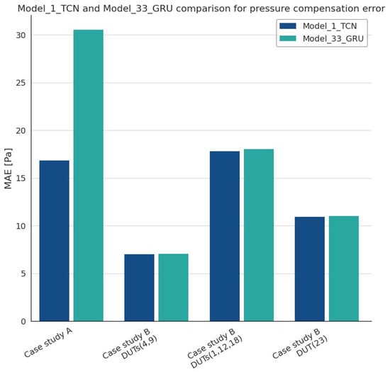
Figure 5.
Performance comparison of model_1_TCN and model_33_GRU.
Figure 5 shows clearly that, for case A, model_1_TCN outperforms model_33_GRU, achieving a lower MAE of 16.85 Pa. In contrast, model_33_GRU exhibits a higher degree of error, with an MAE of 30.54 Pa. This discrepancy underscores the superior accuracy of model_1_TCN in the challenging post-soldering scenario, emphasizing its efficacy in handling drifts introduced by soldering processes.
10. Summary of This Work
This work proposes an answer to the original research question, “How tiny can a machine learning model be designed to provide accurate drift compensation for the use cases in Section 3.2 and Section 3.3?”. In total, 53 different ML/DL models, including TCN, RNN, LSTM, GRU, LMU, RFR, and SVR, have been devised and analyzed. These models were trained and tested on four sets of sensor data generated in STMicroelectronics Laboratories for two case studies: soldering drift and normal usage. For each ML/DL model, two candidates were selected on the basis of the highest ratio between training samples and model parameters and the lowest MAE. The model_1_TCN, model_33_GRU, and model_53_SVR models are present in Table 7, Table 8, Table 9 and Table 10 since they exhibited the lowest MAE values and the highest ratios. In particular, model_1_TCN performs much more accurately than the other TCN models in terms of ratio both for cases A and B, while its MAE remains slightly higher and comparable. Among the RNNs, model_33_GRU performed significantly better than the alternatives and exhibited an MAE slightly greater than model_1_TCN and an approximately 10% lower ratio for case B. Finally, model_53_SVR outperformed all the other models, with ratio values for all the tests that were two orders of magnitude greater and a slightly higher and comparable MAE. However, model_1_TCN and model_33_GRU demonstrated their cheap costs when they were deployed on the STM32U5 tiny MCU, as shown in Table 11, Table 12, Table 13 and Table 14. The TCN and GRU models, indeed, require a number of MACC operations and an inference time two orders of magnitude lower than those of the SVR model, meaning significantly cheaper deployability on resource-constrained devices and usability in tiny applications. The importance of achieving high pressure accuracy with scarce implementation resources is proven, for example, by the model_1_TCN model, so as to be considered within altitude localization applications. It can be approximately calculated that, in the first 1500 m, the pressure decreases by 1 hPa every 8.3 m; at 3000 m, by 1 hPa every 10 m; and at 9000 m, by 1 hPa every 50 m. Since the Burj Khalifa, the highest building in the world, in Dubai, is 828 m tall, the rule of 1 hPa every 8.3 m can be applied. The accuracy of 16.85 Pa for the model_1_TCN model in case study A translates into accuracy of 1.4 m, which is essential for precise sensor localization.
11. Future Perspectives
Although this study focused on devising pre-trained ML/DL solutions suitable to address the drift effects of the thermal stresses affecting pressure measurement accuracy, the achieved results enable accurate re-calibration during the operative life of the MEMS sensor. It has been demonstrated that very tiny ML/DL models can be successfully deployed on low-power and resource-constrained platforms. Given their limited computational complexity and small memory footprint, these results pave the way to cheap, affordable unsupervised learning performed on either sensors or MCUs. These will allow us to reduce the complexity and the effort of generating and handling enormous datasets during the sensor manufacturing, characterization, and validation processes performed in the STMicroelectronics MEMS Sensor Characterization and Measurement Laboratory.
Author Contributions
Conceptualization, D.P., W.B.Y., G.D.L. and P.V.; methodology, D.P., W.B.Y., G.D.L. and P.V.; software, W.B.Y. and P.V.; validation, W.B.Y.; formal analysis, D.P., W.B.Y., G.D.L. and P.V.; investigation, D.P., W.B.Y., G.D.L. and P.V.; resources, D.P., W.B.Y., F.M.A., G.D.L. and P.V.; data curation, W.B.Y. and P.V.; writing—original draft preparation, D.P., W.B.Y., F.M.A., G.D.L. and P.V.; writing—review and editing, D.P., W.B.Y., F.M.A., G.D.L. and P.V.; visualization, D.P., W.B.Y. and P.V.; supervision, D.P. and G.D.L.; project administration, D.P. and G.D.L. All authors have read and agreed to the published version of the manuscript.
Funding
This research received no external funding.
Data Availability Statement
Data sharing is not applicable to this article.
Conflicts of Interest
Author Danilo Pau, Welid Ben Yahmed, and Fabrizio Maria Aymone were employed by the company STMicroelectronics. The remaining authors declare that the research was conducted in the absence of any commercial or financial relationships that could be construed as a potential conflict of interest.
References
- Pressure Sensor Market Size, Share & Trends Analysis Report by Product (Differential, Absolute), by Type (Wireless, Wired), by Technology (Capacitive, Optical), by Application (Oil & Gas, Medical), and Segment Forecasts, 2023–2030; Technical Report; Grand View Research, Inc.: San Francisco, CA, USA, 2023.
- Hajare, R.; Reddy, V.; Srikanth, R. MEMS based sensors—A comprehensive review of commonly used fabrication techniques. Mater. Today Proc. 2022, 49, 720–730. [Google Scholar] [CrossRef]
- Meti, S.; Balavald, K.B.; Sheeparmatti, B. MEMS piezoresistive pressure sensor: A survey. Int. J. Eng. Res. Appl. 2016, 6, 23–31. [Google Scholar]
- Zhou, G.; Zhao, Y.; Guo, F.; Xu, W. A Smart High Accuracy Silicon Piezoresistive Pressure Sensor Temperature Compensation System. Sensors 2014, 14, 12174–12190. [Google Scholar] [CrossRef] [PubMed]
- Rivera, J.; Carrillo, M.; Chacón, M.; Herrera, G.; Bojorquez, G. Self-calibration and optimal response in intelligent sensors design based on artificial neural networks. Sensors 2007, 7, 1509–1529. [Google Scholar] [CrossRef]
- Alzubaidi, L.; Zhang, J.; Humaidi, A.J.; Al-Dujaili, A.; Duan, Y.; Al-Shamma, O.; Santamaría, J.; Fadhel, M.A.; Al-Amidie, M.; Farhan, L. Review of deep learning: Concepts, CNN architectures, challenges, applications, future directions. J. Big Data 2021, 8, 1–74. [Google Scholar] [CrossRef] [PubMed]
- Krizhevsky, A.; Sutskever, I.; Hinton, G.E. ImageNet Classification with Deep Convolutional Neural Networks. In Proceedings of the Advances in Neural Information Processing Systems; Pereira,, F., Burges, C., Bottou, L., Weinberger, K., Eds.; Curran Associates, Inc.: Red Hook, NY, USA, 2012; Volume 25. [Google Scholar]
- Xu, X.; Zhang, Y. Second-hand house price index forecasting with neural networks. J. Prop. Res. 2022, 39, 215–236. [Google Scholar] [CrossRef]
- Zhang, G.; Qi, M. Neural network forecasting for seasonal and trend time series. Eur. J. Oper. Res. 2005, 160, 501–514. [Google Scholar] [CrossRef]
- Cybenko, G. Approximation by superpositions of a sigmoidal function. Math. Control Signals Syst. 1989, 2, 303–314. [Google Scholar] [CrossRef]
- Hornik, K.; Stinchcombe, M.; White, H. Multilayer feedforward networks are universal approximators. Neural Netw. 1989, 2, 359–366. [Google Scholar] [CrossRef]
- Stone, J.O. Air pressure and cosmogenic isotope production. J. Geophys. Res. Solid Earth 2000, 105, 23753–23759. [Google Scholar] [CrossRef]
- Li, B.; Harvey, B.; Gallagher, T. Using barometers to determine the height for indoor positioning. In Proceedings of the International Conference on Indoor Positioning and Indoor Navigation, Montbeliard-Belfort, France, 28–31 October 2013; pp. 1–7. [Google Scholar] [CrossRef]
- Xia, H.; Wang, X.; Qiao, Y.; Jian, J.; Chang, Y. Using multiple barometers to detect the floor location of smart phones with built-in barometric sensors for indoor positioning. Sensors 2015, 15, 7857–7877. [Google Scholar] [CrossRef]
- Licciardo, G.D.; Vitolo, P.; Bosco, S.; Pennino, S.; Pau, D.; Pesaturo, M.; Di Benedetto, L.; Liguori, R. Ultra-Tiny Neural Network for Compensation of Post-soldering Thermal Drift in MEMS Pressure Sensors. In Proceedings of the 2023 IEEE International Symposium on Circuits and Systems (ISCAS), Monterey, CA, USA, 21–25 May 2023; pp. 1–5. [Google Scholar] [CrossRef]
- Vitolo, P.; Pau, D.; Licciardo, G.D.; Pesaturo, M.; Bosco, S.; Pennino, S. Tiny compensation of pressure drift measurements due to long exposures to high temperatures. In Proceedings of the 2023 IEEE International Instrumentation and Measurement Technology Conference (I2MTC), Kuala Lumpur, Malaysia, 22–25 May 2023; pp. 1–5. [Google Scholar] [CrossRef]
- STMicroelectronics. High-Performance MEMS Nano Pressure Sensor: 260–1260 hPa Absolute Digital Output Barometer; STMicroelectronics: Geneva, Switzerland, 2019. [Google Scholar]
- IPC/JEDEC J-STD-020C; Moisture/Reflow Sensitivity Classification for Nonhermetic Solid State Surface Mount Devices. JEDEC Solid State Technology Association: Arlington, VA, USA, 2004.
- Chang, Y.; Cui, X.; Hou, G.; Jin, Y. Calibration of the Pressure Sensor Device with the Extreme Learning Machine. In Proceedings of the 2020 21st International Conference on Electronic Packaging Technology (ICEPT), Guangzhou, China, 12–15 August 2020; pp. 1–5. [Google Scholar] [CrossRef]
- Najar, H. Electrical Only Calibration of Barometric Pressure Sensors Using Machine Learning. In Proceedings of the 2019 20th International Conference on Solid-State Sensors, Actuators and Microsystems & Eurosensors XXXIII (TRANSDUCERS & EUROSENSORS XXXIII), Berlin, Germany, 23–27 June 2019; pp. 1977–1980. [Google Scholar] [CrossRef]
- Patra, J.; Gopalkrishnan, V.; Ang, E.L.; Das, A. Neural network-based self-calibration/compensation of sensors operating in harsh environments [smart pressure sensor example]. In Proceedings of the SENSORS, 2004 IEEE, Vienna, Austria, 24–27 October 2004; Volume 1, pp. 425–428. [Google Scholar] [CrossRef]
- Wu, R.; Li, H.; Gao, L. Research on temperature drift mechanism and compensation method of silicon piezoresistive pressure sensors. AIP Adv. 2023, 13, 035323. [Google Scholar] [CrossRef]
- Ali, I.; Asif, M.; Shehzad, K.; Rehman, M.R.U.; Kim, D.G.; Rikan, B.S.; Pu, Y.; Yoo, S.S.; Lee, K.Y. A Highly Accurate, Polynomial-Based Digital Temperature Compensation for Piezoresistive Pressure Sensor in 180 nm CMOS Technology. Sensors 2020, 20, 5256. [Google Scholar] [CrossRef] [PubMed]
- Futane, N.; Chowdhury, S.R.; Chowdhury, C.R.; Saha, H. ANN based CMOS ASIC design for improved temperature-drift compensation of piezoresistive micro-machined high resolution pressure sensor. Microelectron. Reliab. 2010, 50, 282–291. [Google Scholar] [CrossRef]
- Soy, H.; Toy, İ. Design and implementation of smart pressure sensor for automotive applications. Measurement 2021, 176, 109184. [Google Scholar] [CrossRef]
- Zou, M.; Xu, Y.; Jin, J.; Chu, M.; Huang, W. Accurate Nonlinearity and Temperature Compensation Method for Piezoresistive Pressure Sensors Based on Data Generation. Sensors 2023, 23, 6167. [Google Scholar] [CrossRef]
- Sarmad, M.; Fatima, M.; Tayyub, J. Reducing Energy Consumption of Pressure Sensor Calibration Using Polynomial HyperNetworks with Fourier Features. Proc. Aaai Conf. Artif. Intell. 2022, 36, 12145–12153. [Google Scholar] [CrossRef]
- Xie, W.; Bai, P. A pressure sensor calibration model based on Support Vector Machine. In Proceedings of the 2012 24th Chinese Control and Decision Conference (CCDC), Taiyuan, China, 23–25 May 2012; pp. 3239–3242. [Google Scholar] [CrossRef]
- Chuan, Y.; Chen, L. The Application of Support Vector Machine in the Hysteresis Modeling of Silicon Pressure Sensor. IEEE Sens. J. 2011, 11, 2022–2026. [Google Scholar] [CrossRef]
- Wang, H.; Li, J. Machine Learning and Swarm Optimization Algorithm in Temperature Compensation of Pressure Sensors. Sensors 2022, 22, 8309. [Google Scholar] [CrossRef]
- Li, J.; Zhang, C.; Zhang, X.; He, H.; Liu, W.; Chen, C. Temperature Compensation of Piezo-Resistive Pressure Sensor Utilizing Ensemble AMPSO-SVR Based on Improved Adaboost.RT. IEEE Access 2020, 8, 12413–12425. [Google Scholar] [CrossRef]
- Zhao, X.; Li, P.; Xiao, K.; Meng, X.; Han, L.; Yu, C. Sensor Drift Compensation Based on the Improved LSTM and SVM Multi-Class Ensemble Learning Models. Sensors 2019, 19, 3844. [Google Scholar] [CrossRef]
- Wang, T.; Liu, P.; Zhang, W.; Jia, X.; Wang, Y.; Yang, J. Calibration of Multi-dimensional Air Pressure Sensor Based on LSTM. In Proceedings of the Artificial Intelligence and Security; Sun, X., Zhang, X., Xia, Z., Bertino, E., Eds.; Springer: Cham, Switzerland, 2022; pp. 532–543. [Google Scholar]
- Chaudhuri, T.; Wu, M.; Zhang, Y.; Liu, P.; Li, X. An Attention-Based Deep Sequential GRU Model for Sensor Drift Compensation. IEEE Sens. J. 2021, 21, 7908–7917. [Google Scholar] [CrossRef]
- Almassri, A.M.M.; Wan Hasan, W.Z.; Ahmad, S.A.; Shafie, S.; Wada, C.; Horio, K. Self-Calibration Algorithm for a Pressure Sensor with a Real-Time Approach Based on an Artificial Neural Network. Sensors 2018, 18, 2561. [Google Scholar] [CrossRef]
- Ho, T.K. Random decision forests. In Proceedings of the 3rd International Conference on Document Analysis and Recognition, Montreal, QC, Canada, 14–16 August 1995; Volume 1, pp. 278–282. [Google Scholar] [CrossRef]
- Awad, M.; Khanna, R.; Awad, M.; Khanna, R. Support vector regression. In Efficient Learning Machines: Theories, Concepts, and Applications for Engineers and System Designers; Apress Open, Apress Media, LLC: New York, NY, USA, 2015; pp. 67–80. [Google Scholar]
- Alade, I.O.; Zhang, Y.; Xu, X. Modeling and prediction of lattice parameters of binary spinel compounds (AM2X4) using support vector regression with Bayesian optimization. New J. Chem. 2021, 45, 15255–15266. [Google Scholar] [CrossRef]
- Cao, L.; Tay, F. Financial Forecasting Using Support Vector Machines. Neural Comput. Appl. 2001, 10, 184–192. [Google Scholar] [CrossRef]
- Zhang, Y.; Xu, X. Disordered MgB2 superconductor critical temperature modeling through regression trees. Phys. C Supercond. Appl. 2022, 597, 1354062. [Google Scholar] [CrossRef]
- Choubin, B.; Zehtabian, G.; Azareh, A.; Rafiei Sardooi, E.; Sajedi Hosseini, F.; Kisi, O. Precipitation forecasting using classification and regression trees (CART) model: A comparative study of different approaches. Environ. Earth Sci. 2018, 77, 314. [Google Scholar] [CrossRef]
- Lea, C.; Vidal, R.; Reiter, A.; Hager, G.D. Temporal convolutional networks: A unified approach to action segmentation. In Proceedings of the Computer Vision–ECCV 2016 Workshops, Amsterdam, The Netherlands, 8–10, 15–16 October 2016; Part III 14. Springer: Berlin/Heidelberg, Germany, 2016; pp. 47–54. [Google Scholar]
- Rumelhart, D.E.; Hinton, G.E.; Williams, R.J. Learning Internal Representations by Error Propagation; MIT Press: Cambridge, MA, USA, 1986. [Google Scholar]
- Hochreiter, S.; Schmidhuber, J. Long Short-Term Memory. Neural Comput. 1997, 9, 1735–1780. [Google Scholar] [CrossRef]
- Cho, K.; van Merriënboer, B.; Gulcehre, C.; Bahdanau, D.; Bougares, F.; Schwenk, H.; Bengio, Y. Learning Phrase Representations using RNN Encoder–Decoder for Statistical Machine Translation. In Proceedings of the 2014 Conference on Empirical Methods in Natural Language Processing (EMNLP), Doha, Qatar, 25–29 October 2014; Moschitti, A., Pang, B., Daelemans, W., Eds.; Association for Computational Linguistics: Stroudsburg, PA, USA, 2014; pp. 1724–1734. [Google Scholar] [CrossRef]
- Voelker, A.R.; Kajić, I.; Eliasmith, C. Legendre Memory Units: Continuous-Time Representation in Recurrent Neural Networks. Adv. Neural Inf. Process. Syst. 2019, 32, 15544–15553. [Google Scholar]
- Kingma, D.P.; Ba, J. Adam: A method for stochastic optimization. arXiv 2014, arXiv:1412.6980. [Google Scholar]
Disclaimer/Publisher’s Note: The statements, opinions and data contained in all publications are solely those of the individual author(s) and contributor(s) and not of MDPI and/or the editor(s). MDPI and/or the editor(s) disclaim responsibility for any injury to people or property resulting from any ideas, methods, instructions or products referred to in the content. |
© 2023 by the authors. Licensee MDPI, Basel, Switzerland. This article is an open access article distributed under the terms and conditions of the Creative Commons Attribution (CC BY) license (https://creativecommons.org/licenses/by/4.0/).