Research on a High-Performance Rock Image Classification Method

Abstract

Efficient and convenient rock image classification methods are important for geological research. They help in identifying and categorizing rocks based on their physical and chemical properties, which can provide insights into their geological history, origin, and potential uses in various applications. The classification and identification of rocks often rely on experienced and knowledgeable professionals and are less efficient. Fine-grained rock image classification is a challenging task because of the inherent subtle differences between highly confusing categories, which require a large number of data samples and computational resources, resulting in low recognition accuracy, and are difficult to apply in mobile scenarios, requiring the design of a high-performance image processing classification architecture. In this paper we design a knowledge distillation and high-accuracy feature localization comparison network (FPCN)-based learning architecture for generating small high-performance rock image classification models. Specifically, for a pair of images, we interact with the feature vectors generated from the localized feature maps to capture common and unique features, let the network focus on more complementary information according to the different scales of the objects, and then the important features of the images learned in this way are made available for the micro-model to learn the critical information for discrimination via model distillation. The proposed method improves the accuracy of the micro-model by 3%.

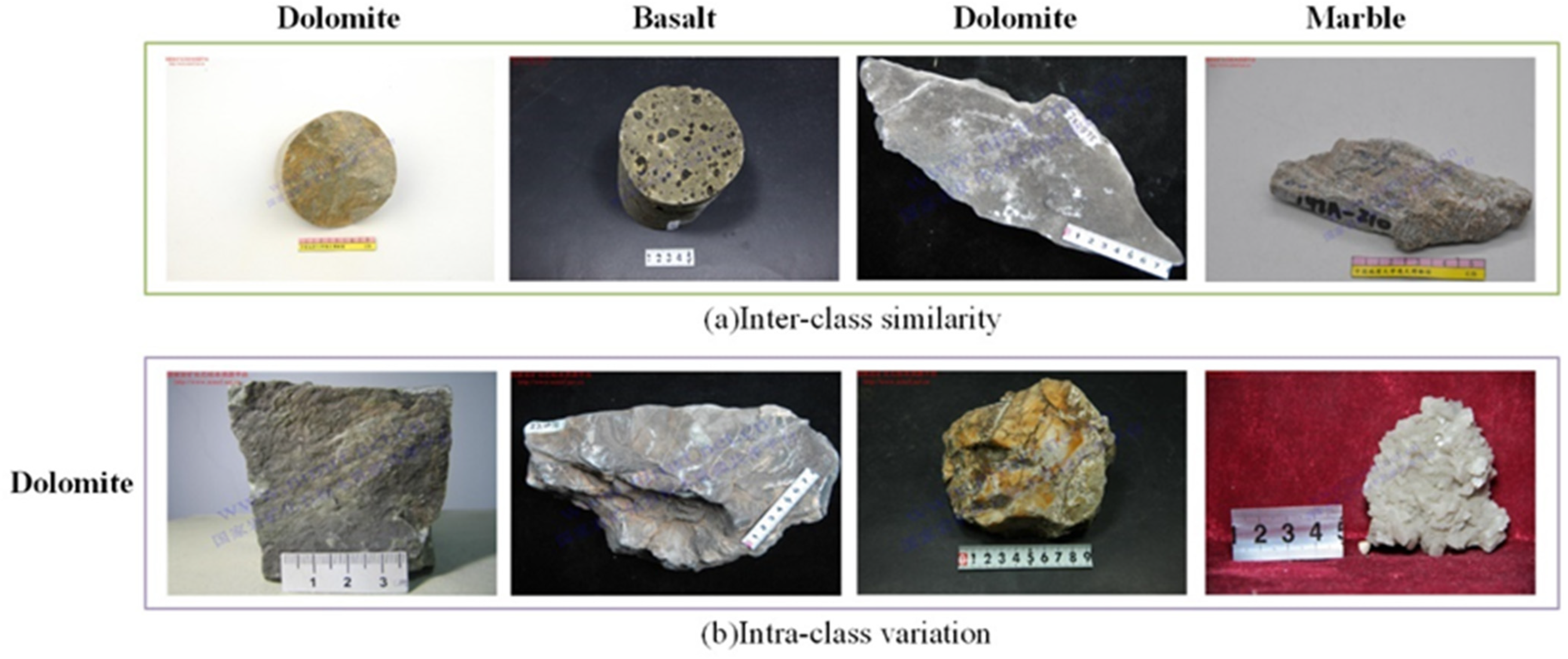
1. Introduction

The identification of rock types is an important part of geological research, and accurate and efficient rock image classification is of great importance. The classification of rock images is a fine-grained visual classification task. Although convolutional neural networks (CNNs) have achieved remarkable results in recent years for general image classification [1], the fine-grained classification of rock images is still a challenging task due to the great similarity between subclasses.

In recent years, some studies related to automatic rock image classification have been proposed and some progress has been made. Chatterjee et al. [2,3,4] extracted the texture features of rock images and used a support vector machine-based method to perform regression prediction based on texture features. Liang et al. [5] used a convolutional neural network-based approach, Guojian [6] proposed a residual network based on a rock slice image classification method, and Pascual et al. [7] used a three-layer convolutional neural network (CNN) approach to classify rock images to improve classification accuracy. To enhance discriminative feature learning and to alleviate the overfitting problem, data augmentation has also been applied in some fine-grained image classification schemes. There are essentially three modes of data augmentation: (1) Image mixing [8]. The training data are enhanced by blending images/patches and labels from two samples. (2) Image resampling [9], which is a non-uniform image sampling method and is usually guided by an attention map. (3) Image cropping [10]. Image cropping is a widely used enhancement method that is suitable for different visual scales and easy to apply. The cropped images may contain too much irrelevant information, which may aggravate the overfitting problem.

Zhao [11] proposes rock image data expansion and data enhancement based on a generative adversarial network (GAN) from the perspective of rock image samples to make the trained model better by using better data samples.

As shown in Figure 1, the difficulties in fine-grained classification of rock images are (1) the existence of large intra-class variance, where images of similar rocks have different backgrounds, different perspectives, and different scales of rock subjects, resulting in large feature differences between similar samples; (2) small inter-class variance, where there are visually very similar samples between rock subclasses, which have similar color, texture, and shape, relying on subtle differences to be distinguished; (3) in scenarios such as field exploration, the rock image recognition conditions are restricted, including shooting clarity and mobile device performance limitations, and it is also challenging to ensure the model efficiency of rock classification.

To address these issues, this study designs a knowledge distillation and high-accuracy feature-positioning comparison network (FPCN)-based learning architecture for generating high-performance rock image classification micro-models.

(1) It obtains the basic regions of the rock body using the feature maps generated by the pre-trained model without the additional annotation of the rock image location frames;

(2) It learns key features of rock image types using a self-supervised learning approach based on intra- and inter-class contrast learning of rock images and filtering irrelevant contrast information;

(3) The rock classification baseline models of different sizes are tested, the accuracy, scale, and efficiency are tested, and the accuracy of the small models is improved via distillation.

Our source code is available at https://github.com/TohsakaRin404/Feature-Positioning-Contrast-Network (accessed on 7 November 2023).

2. Related Work

In recent years, there have been many works on fine-grained image classification, and the main proposed ideas and methods of these works are summarized and discussed in the following.

2.1. Target Object Positioning

Since the target to be classified is at an arbitrary position in the image and does not always fill the whole image, locating the classification target can exclude the interference of other elements in the background of the image. Background modeling algorithms [12] are a class of typical algorithms in unsupervised learning target detection methods. The basic principle is to use video images or multiple consecutive pieces of image information to construct a background image model that can accurately describe the background information, and then use the background image model for comparison with the original image to extract the target in the image. Some localization methods determine the object location using features generated by convolutional neural networks [13,14,15,16,17]. R-CNN [13] proposes the generation of several alternative regions on the detected image using a selective search [18] and extracts the corresponding feature vector from each region, and then the most correctly classified region is identified as the target region. Such approaches require manual annotation of the part frames of the manually annotated objects and consume a lot of time and computational resources. Therefore, weakly supervised approaches to localization [19,20,21,22] have been proposed: RA-CNN [19] continuously zooms in on the region of interest in the convolutional layer and uses the zoomed image as input to obtain the classification result as part of the final result. S3N [21] determines the object region using the maximum position of the image response to each category. This type of method achieves good results under the condition that location frame labeling is not required, but it requires a two-stage process of localization–classification, and there are multiple inputs and multiple networks, which may lead to a complex and inefficient model.

2.2. Learning More Discriminating Features

High-quality features are especially important in fine-grained image classification because the differences between fine-grained images are often small. The construction of robust feature representations has been widely studied for fine-grained image classification. The earliest representative method is Bilinear CNN [23], which aggregates features extracted by two CNNs to generate higher order features that describe pairs of features. Subsequent methods inspired by this include the methods in [21,22,24,25,26,27,28], which set multiple feature extraction modules and for each module input cropped, erased, masked, and zoomed-in multi-view image samples. Such methods extracted richer feature representations and achieved better results, but were unable to determine which features truly distinguish classes from each other and the unique features within classes. Rao [29] proposed an attention learning approach based on causal inference to encourage networks to learn more effective visual attention. Inspired by this, fine-grained image classification methods based on contrast learning were proposed using CIN [25] to exploit channel correlations between samples to pull positive pairs closer while pushing away negative pairs through channel interactions, and PCA-Net [26] and API-Net [27] to learn common and difference features through channel interactions with simultaneous input of positive/negative sample pairs. The fine-grained image classification method based on contrast learning achieves the best results so far, but the problem remains that similar features of similar samples and different features of dissimilar samples are used as the basis for discrimination, and these features are not the right basis on which to distinguish them. For example, when using two images obtained from two different birds under the same sky with the same sky background color and light, where both have an airplane in the background, the existing models may classify the two images as the same type. In this paper, we try to delineate the contrast region using a weakly supervised localization method to allow the model to learn the truly critical unique and differential features.

One of the major challenges of deep learning models is that they are difficult to deploy on resource-constrained devices, such as embedded devices and mobile devices, due to resource capacity limitations. In recent years, a large number of large model compression and acceleration techniques have been proposed, including knowledge distillation, where a small student model can efficiently learn from a large teacher model. Hinton’s team’s proposed response-based knowledge distillation [30] pioneered the field of knowledge distillation, followed by feature-based knowledge distillation. Since then, feature-based and relation-based knowledge distillation algorithms have been proposed. Using complex fine-grained image recognition models as teacher models to train tiny models that can be applied to mobile devices can improve the model performance without changing the model size.

3. Method

In this section, we propose the feature-positioning contrast network (FPCN) for fine-grained rock image classification. As shown in Figure 2, the model is divided into three main parts: object positioning, part contrast learning and optimization loss. We optimize the student model training process based on the FPCN inference.

3.1. Object Positioning

The purpose of the main object localization module is to determine the approximate area in the image where the object is located. Due to the interference of invalid contrast information generated by the background or other objects, the localization region can help focus on the critical contrast regions in the contrast module. Our proposed feature map maximum region detection approach does not require additional annotation of the location frame, and the target location is obtained by generating the highlighted connected regions of the feature map using a pre-trained image detection network.

Given an input image $I$, $\mathit{F}\in {ℝ}^{H\times W\times C}$ denotes the feature map obtained after the last convolutional layer of the backbone, and $H,W,C$ denote the height, width, and number of channels of the feature map, respectively, with $\mathit{L}\in {ℝ}^{H\times W}$ denoting the feature map of a single channel, and the feature map of each channel is overlayed to obtain the activation map $\mathit{A}$ of $I$, as shown in Equation (1).

$$\mathit{A}={\displaystyle \sum _{i=0}^C{\mathit{L}}_{\mathit{i}}}$$

(1)

To obtain the pixel regions with significant activation values, the average value of the activated pixel values is calculated as in Equation (2).

$$\overline{\mathrm{A}}=\frac{{\displaystyle \sum _{x=1,y=1}^{W,H}\mathit{A}(x,y)}}{W\times H}$$

(2)

$A(x,y)$ denotes the activation value of a pixel in the activation map and $\overline{\mathrm{A}}$ is used as a threshold to determine the object position, thus obtaining an approximate mask map of the object target according to Equation (3).

$$\mathit{M}(x,y)=\{\begin{array}{l}1,\mathrm{if}\mathit{A}(x,y)\ge \overline{A}\\ \theta ,0\le \theta <1,\mathrm{else}\end{array}$$

(3)

Considering that the objects in the image take up different ratios of the complete image with different scales, and the unlabeled localization method may not be accurate enough, retaining part of the features outside the mask helps to supplement the effective information. $\theta$ indicates the ratio of features retained outside the object. The simplest explanation is that the smaller the number of pixels that are occupied by the object, the lower the amount of information it contains and the lower the amount of complementary information that is needed, and the area share of the target subject in the figure is expressed by $\alpha$ as shown in Equation (4).

$$\alpha =\frac{{\displaystyle \sum _{x=1,y=1}^{W,H}\mathit{M}(x,y)}}{W\times H}$$

(4)

$\alpha$ denotes the mask intensity, balancing the ratio of subject information and extra-object supplementary information. The experiments in Section 4.3 list the accuracy of the model with different parameters $\alpha$. The mask is overlaid on the feature map to obtain a feature map that preserves the object feature, denoted by ${\mathit{F}}_{\mathit{mask}}$.

$${\mathit{F}}_{\mathit{mask}}=\alpha \odot \mathit{F}\odot \mathit{M}$$

(5)

In Equation (5), $\odot$ indicates multiplication by elements. When the ratio of objects in the image is large, the feature map focuses more on the object itself; when the ratio is smaller, the feature map retains more features outside the object. This ensures that the features outside the object in the image are utilized while focusing on the object itself when the target object is small or not completely accurate in positioning.

3.2. Part Comparison Learning

In order for the model to learn common features within classes and differential features between classes, we propose a between-objects comparison learning module. For any pair of image samples (including the cases of the same class and different classes), a fused vector ${\mathit{X}}_{\mathit{f}}\in R^{D\times C}$, shown in Equation (6), is learned by a trainable multi-layer perceptron with the help of the mask feature maps obtained by the localization module, which contain the unique features and common features of the sample pairs. Specifically, we use ${\mathit{F}}_{\mathit{A}}$ and ${\mathit{F}}_{\mathit{B}}$ to represent the mask feature maps generated with a pair of samples and ${\mathit{X}}_{\mathit{a}}\in R^{D\times C}$ and ${\mathit{X}}_{\mathit{b}}\in R^{D\times C}$ to represent the average pooled feature vectors, perform the global average pooling (GAP) operation on ${\mathit{F}}_{\mathit{A}}$ and ${\mathit{F}}_{\mathit{B}}$ to obtain the object feature representations ${\mathit{X}}_{\mathit{a}}$ and ${\mathit{X}}_{\mathit{b}}$ as in Equation (7), and use $j=1,2\dots C$ to represent the feature map corresponding to the channel of the $j\mathrm{th}$ pair.

$${\mathit{X}}_{\mathit{f}}=\mathrm{MLP}(concat({\mathit{X}}_{\mathit{a}},{\mathit{X}}_{\mathit{b}}))$$

(6)

$${\mathit{X}}_{\mathit{A}\mathit{j}}={\displaystyle \sum _{x=1,y=1}^{W,H}{\mathit{F}}_{\mathit{A}\mathit{j}}(x,y)}$$

(7)

The interaction of ${\mathit{X}}_{\mathit{f}}$ with ${\mathit{X}}_{\mathit{a}}$ and ${\mathit{X}}_{\mathit{b}}$ activates the unique and common features of the corresponding feature vectors of the samples, as shown in Equations (8) and (9). The explanation for this design is that the fused feature vectors point out the key contrast features and the sample feature vectors retain this key contrast information when interacting with each sample.

$${\mathit{X}}_{\mathit{a}\mathit{f}}={\mathit{X}}_{\mathit{a}}\odot {\mathit{X}}_{\mathit{f}}$$

(8)

$${\mathit{X}}_{\mathit{b}\mathit{f}}={\mathit{X}}_{\mathit{b}}\odot {\mathit{X}}_{\mathit{b}\mathit{f}}$$

(9)

3.3. Model Training Optimization

Due to the problem of large intra-class variance in fine-grained image classification, relying only on the cross-entropy loss function to pull apart the inter-class distance in the feature space may also create the problem of overlapping decision boundaries of different classes. Moreover, for model stability, the attention maps of each channel are expected to provide specific attention patterns, e.g., in rock classification, one of the attention maps focuses on color features and the other on rock texture features; however, the supervision of classification loss alone does not guarantee this. To make the intra-class samples more aggregated, center loss is introduced [31], which initializes an intra-class center for each class and brings the feature vectors of this class samples closer to the center; each class center is determined by the feature vectors of this class and is continuously updated during training, and all images in each training iteration help to update their corresponding center feature vectors. The initial center of a class is denoted by $\mathit{c}\in R^{D\times C}$, the center of a round is updated by ${\mathit{c}}^{\prime }$, and the update process is as in Equation (10).

$${\mathit{c}}^{\prime }=\mathit{c}+\frac{{\displaystyle \sum _{i=1}^m{\mathit{x}}_{\mathit{i}}-\mathit{c}}}{m}$$

(10)

${\mathit{x}}_{\mathit{i}}$ denotes the feature vector of the $i\mathrm{th}$ sample of the category $\mathit{c}$, and $m$ denotes the number of feature vectors of the category $\mathit{c}$. The central loss function for each epoch is shown in Equation (11), where $\left|\right|·|{|}_2^2$ denotes the $L_2$ norm and $\mathit{c}$ denotes the class center vector of the category $\mathit{c}$ under the current epoch.

$${ℒ}_{center}=\frac{1}{2}{\displaystyle \sum _{i=1}^m\left|\right|{\mathit{x}}_{\mathit{i}}-\mathit{c}|{|}_2^{}}$$

(11)

The whole model optimization process in the training phase is shown in Equation (12). ${ℒ}_{class}$ uses a cross-entropy loss function in category predictions, and the overall loss is expressed as the sum of the classification loss and the central loss. $\lambda$ is the hyperparameter to balance the two losses, which is set to 0.5 based on experimental experience.

$$ℒ={ℒ}_{class}+\lambda {ℒ}_{center}$$

(12)

3.4. Knowledge Distillation Training Optimization

We use $y_i$ to denote the corresponding value of the teacher network’s prediction class and $T$ to denote the distillation temperature, which weakens the predicted value difference between the target and non-target classes, and helps the student model to learn the distribution of the predicted values as shown in Equation (13).

$$p(y_i,T)=soft\max (y_i/T)$$

(13)

In order to reduce the difference between the teacher model and the student model, Kullback–Leibler divergence (KL) was used to measure the difference between the predictions of the two models and minimize this value as shown in Equation (14), where ${\mathit{p}}_{\mathit{i}}^{\mathit{T}},{\mathit{p}}_{\mathit{i}}^{\mathit{S}}$ denote the predicted logits of class i in the teacher model and student model, respectively. KL divergence describes the similarity in distribution of two models by optimizing it to become smaller to make the student model similar to the teacher model.

$${ℒ}_1=KL(\mathit{p}({\mathit{y}}_{\mathit{teacher}},\mathit{T}),\mathit{p}({\mathit{y}}_{\mathit{student}},\mathit{T}))={\displaystyle \sum _{\mathit{i}=1}^m{\mathit{p}}_{\mathit{i}}^{\mathit{T}}\log (\frac{{\mathit{p}}_{\mathit{i}}^{\mathit{T}}}{{\mathit{p}}_{\mathit{i}}^{\mathit{S}}})}$$

(14)

4. Experiments and Discussions

4.1. Datasets and Implementation Details

The rock image dataset used in this paper is a sample of rocks from the Geological Museum taken under different perspectives and lights, including three types of dolomite, marble, and basalt with a total of 39,620 rock images, all with a resolution higher than 448 × 448 as shown in

Table 1. Fine-grained rock dataset.

Rock Type	Number
dolomite	7924
marble	11,658
basalt	19,678

.

First, we resized each image to 448 × 448 specifically, by performing random cropping during training and center cropping during testing, as the input to the FPCN. We used ResNet-101, pre-trained on ImageNet, as the backbone network for the proposed model. We did not use any annotation information other than the category labels of the images during training. In this paper, we implemented the proposed model using the Pytorch deep learning framework and trained it on a computer with an RTX A5000 (24 GB) GPU and 42 GB memory. The training process used the stochastic gradient optimization algorithm (SGD) with a momentum of 0.9 and training rounds were set to 100 (reached convergence in 80–90 epochs in the actual training process) with a batch size of 42 (14 images of each type) and an initial learning rate of 0.01.

When constructing the input image pairs, their mask feature maps and comparison vectors were generated for any two samples in each batch, and the overall optimization of the model was performed. Intuitively, the larger the number of samples in each batch, the better the comparison. The training results of different batch sizes are tested in Section 4.2, but considering that setting a larger batch size will consume a lot of storage space and computational resources, and the batch size set in this paper achieved quite good results, the model effect under larger batches was not tested.

4.2. Experimental Results

As shown in

Table 2. Comparison results on rock dataset.

Basic Model	Train Acc@1 (%)	Test Acc@1 (%)	Backbone
AlexNet	96.8	73.1
LeNet	50.1	50.5
GoogLeNet	86.6	76.3
VGG16	76.1	72.3
ResNet-50	79.6	72.4
Fine-Grained Model
Bilinear CNN (2015)	85.4	85.3	VGG16
PCA-Net (2021)	94.9	90.8	ResNet-101
API-Net (2020)	99.8	91.2	ResNet-101
MMAL-Net (2021)	99.7	91.9	ResNet-50
Ours	99.8	93.1	ResNet-101

, the proposed method in this paper is compared with the basic and fine-grained classification models for image classification, and the proposed method in this paper achieves the best accuracy of 93.1% on the rock image dataset used. Train Acc@1 and Test Acc@1 denote the probability that the predicted class with the highest probability is the true label in the training and test datasets. Compared with the suboptimal PCA-Net and API-Net, two models based on contrast learning, our method adds an half-supervised object localization module to achieve filtering of invalid contrast information and is more effective; compared with MMAL-Net’s multi-view learning approach of localizing both objects and multiple parts, our method considers a soft mask according to the ratio of objects to supplement more feature information in the case of inaccurate target object localization or small target objects.

4.3. Ablation Study

We studied the impact of the key design in the proposed method on the results. To verify the validity of the key components in the model, we conducted an ablation study using ResNet-101 on a fine-grained rock dataset, as shown in

Table 3. Ablation study on the effect of each design on rock dataset.

Area Mask	Center Loss	Area Scale ($\mathit{\alpha }$)	Acc@1 (%)
√			92.0
	√		91.2
√		√	92.2
√	√		92.8
√	√	√	93.1

. Since the area share weights ($\alpha$) depend on the mask module, there was no single test of its ablation. The experiments show that the localization mask module has the largest impact on the results, with a 1% improvement without the introduction of other modules. The accuracy is also improved in the two cases where $\alpha$ is introduced in the third and fifth rows of the table, indicating the presence of insufficient feature information due to small target objects or inaccurate localization in the localization module.

We also studied the effect of the number of image pairs in a single batch on the results. As shown in Figure 3, increasing the number of image pairs in all three models results in a great improvement in the accuracy, indicating that the model learns more information about the contrast features and is able to correctly categorize more indistinguishable images. In the process of increasing the number of contrast samples, the method we proposed outperforms the other two classification models based on contrast learning. The possible reasons for this are the following: when the contrast samples are small, the model can receive less feature information, and the masked feature map contains insufficient information, which limits the number of features extracted by the network; when the contrast samples are sufficient, the model extracts a large number of contrast features, which include wrong contrast features (e.g., the same background in similar images), while our proposed model can filter more critical information from a large number of contrast features through object localization, achieving better results.

We studied the effect of mask intensity $\alpha$ on the enhancement in image classification at different scales. We divided the test set into four parts according to the area ratio generated by the localization module (object ratio <25%, 25–50%, 50–75%, >75% of the image) and counted the changes in their accuracy rates with $\alpha$/without $\alpha$, respectively, as shown in Figure 4. $\alpha$ is smaller when the target object ratio is smaller, retains more feature information outside the object, and the accuracy improvement is greater when there is almost no problem of insufficient feature information or inaccurate localization when the target object occupancy is larger, so the localization classification effect is almost unchanged, and the experimental results proved the effectiveness of the design mask strength $\alpha$.

4.4. Visualization

To further evaluate the effectiveness of our method, we visualized images of fine-grained rock datasets using Grad-CAM [32]. Gradient CAM is formed via a weighted summation of the feature maps, which shows the importance of each region for its classification. We compared the visualization results of our method with the base model (ResNet-101), as shown in Figure 5. It can be observed that the base model will be interested in focusing on the wrong contrast information in the background. Our method can learn more rich and discriminative features, especially those centered on the target subject. Because our method can focus attention on the internal regions of the object, it can make the prediction more comprehensive and capture not only the salient features but also the subtle fine-grained features.

4.5. Small Model Distillation Effect

The results of training the small student model with FPCN as the teacher model are shown in

Table 4. Distillation improvements on small models.

Models		Params	FLOPs	Inference Time (ms)	ACC@1 (%) Baseline	Acc@1 (%) Distilled
(Teacher)	FPCN	46.06 M	28,210 M	13.98	93.1
(Student)	ResNet18	11.89 M	7294 M	2.61	73.8	74.7 (+0.9)
(Student)	ResNet34	22.00 M	14,713 M	5.63	74.7	76.1 (+1.4)
(Student)	ResNet50	25.76 M	16,529 M	7.50	76.5	77.1 (+0.6)
(Student)	MobileNetV1	4.2 M	1080 M	0.82	68.7	71.1 (+2.4)
(Student)	MobileNetV2	3.4 M	1080 M	0.64	70.9	73.5 (+2.6)
(Student)	ShuffleNet(V2)	3.4 M	947 M	0.73	70.5	73.6 (+3.1)

. Each column represents each parameter of the different models, including the number of total model parameters, the number of floating-point operations, the inference time per image, and the accuracy of the test set for training directly and incorporating knowledge distillation on the rock image dataset. The accuracy of the mini-model distilled using the knowledge of the FPCN model is higher than that of the baseline model, which achieves a balance between model efficiency and effectiveness.

5. Conclusions

In this paper, we propose a knowledge distillation and high-accuracy feature localization comparison network (FPCN)-based learning architecture for generating high-performance rock image classification micro-models. To learn more effective contrast feature representation, we use a feature map maximum region detection approach to obtain contrast information about the target region without additional annotation of the location frame. For better intra-class and inter-class contrast feature learning, our FPCN is dynamically tuned depending on the proportion of target objects. From the experimental results, the proposed FPCN model achieves the highest accuracy and proves that the part contrast is superior to the complete image. The knowledge distillation in the FPCN enables the small model to improve in accuracy. In future work, we will add more image sets of rock types to prove that the model works on more complex data. In addition, the improved small model still has some difference in accuracy from the large model, which to some extent indicates that the learning effect of the small model is average or that there is parameter saturation. We will carry out research on better learning architectures or compression methods for the large model in the future to make it easier to be deployed on mobile devices suitable for field geological surveys.

References

- He, K.; Zhang, X.; Ren, S.; Sun, J. Deep residual learning for image recognition. In Proceedings of the CVPR, Las Vegas, NV, USA, 27–30 June 2016; pp. 770–778. [Google Scholar]
- Chatterjee, S. Vision-based rock-type classification of limestone using multi-class support vector machine. Appl. Intell. 2013, 39, 14–27. [Google Scholar] [CrossRef]
- Deng, C.; Pan, H.; Fang, S.; Konaté, A.A.; Qin, R. Support vector machine as an alternative method for lithology classification of crystalline rocks. J. Geophys. Eng. 2017, 14, 341–349. [Google Scholar] [CrossRef]
- Perez, C.A.; Saravia, J.A.; Navarro, C.F.; Schulz, D.A.; Aravena, C.M.; Galdames, F.J. Rock lithological classification using multi-scale Gabor features from sub-images, and voting with rock contour information. Int. J. Miner. Process. 2015, 144, 56–64. [Google Scholar] [CrossRef]
- Liang, Y.; Cui, Q.; Luo, X.; Xie, Z. Research on Classification of Fine-Grained Rock Images Based on Deep Learning. Comput. Intell. Neurosci. 2021, 2021, 5779740. [Google Scholar]
- Guojian, C.; Peisong, L. Rock thin-section image classification based on residual neural network. In Proceedings of the 2021 6th International Conference on Intelligent Computing and Signal Processing (ICSP), Xi’an, China, 9–11 April 2021; pp. 521–524. [Google Scholar]
- Pascual, A.; Lei, S.; Szoke-Sieswerda, J.; Mcisaac, K.; Osinski, G. Towards natural scene rock image classification with convolutional neural networks. In Proceedings of the 2019 IEEE Canadian Conference of Electrical and Computer Engineering (CCECE), Edmonton, AB, Canada, 5–8 May 2019; pp. 1–4. [Google Scholar]
- Yun, S.; Han, D.; Oh, S.J.; Chun, S.; Choe, J.; Yoo, Y. Cutmix: Regularization strategy to train strong classifiers with localizable features. In Proceedings of the IEEE/CVF International Conference on Computer Vision, Seoul, Republic of Korea, 27 October–2 November 2019. [Google Scholar]
- Baboo; Santhosh, S.; Devi, M.R. An analysis of different resampling methods in Coimbatore, District. Glob. J. Comput. Sci. Technol. 2010, 10, 61–66. [Google Scholar]
- Yan, J.; Lin, S.; Kang, S.B.; Tang, X. Learning the change for automatic image cropping. In Proceedings of the IEEE Conference on Computer Vision and Pattern Recognition, Portland, OR, USA, 23–28 June 2013. [Google Scholar]
- Zhao, G.; Cai, Z.; Wang, X.; Dang, X. GAN Data Augmentation Methods in Rock Classification. Appl. Sci. 2023, 13, 5316. [Google Scholar] [CrossRef]
- Zin, T.T.; Tin, P.; Toriu, T.; Hama, H. Background modeling using special type of Markov Chain. IEICE Electron. Express 2011, 8, 1082–1088. [Google Scholar] [CrossRef]
- Girshick, R.; Donahue, J.; Darrell, T.; Malik, J. Rich feature hierarchies for accurate object detection and semantic segmentation. In Proceedings of the IEEE Conference on Computer Vision and Pattern Recognition, Columbus, OH, USA, 23–28 June 2014; pp. 580–587. [Google Scholar]
- Lin, D.; Shen, X.; Lu, C.; Jia, J. Deep LAC: Deep localization, alignment and classification for fine-grained recognition. In Proceedings of the IEEE Conference on Computer Vision and Pattern Recognition, 7–12 June 2015; pp. 1666–1674. [Google Scholar]
- Zhang, N.; Donahue, J.; Girshick, R.B.; Darrell, T. Part-based R-CNNs for fine-grained category detection. In Proceedings of the Computer Vision–ECCV 2014: 13th European Conference, Zurich, Switzerland, 6–12 September 2014; pp. 1173–1182. [Google Scholar]
- Zhang, H.; Xu, T.; Elhoseiny, M.; Huang, X.; Zhang, S.; Elgammal, A.; Metaxas, D. SPDA-CNN: Unifying semantic part detection and abstraction for fine-grained recognition. In Proceedings of the CVPR, Las Vegas, NV, USA, 27–30 June 2016; pp. 1143–1152. [Google Scholar]
- Huang, S.; Xu, Z.; Tao, D.; Zhang, Y. Part-stacked CNN for fine-grained visual categorization. In Proceedings of the 2016 IEEE Conference on Computer Vision and Pattern Recognition, CVPR 2016, Las Vegas, NV, USA, 27–30 June 2016; pp. 1173–1182. [Google Scholar]
- Uijlings, J.; van de Sande, K.; Gevers, T.; Smeulders, A. Selective search for object recognition. Int. J. Comput. Vis. 2013, 104, 154–171. [Google Scholar] [CrossRef]
- Fu, J.; Zheng, H.; Mei, T. Look closer to see better: Recurrent attention convolutional neural network for fine-grained image recognition. In Proceedings of the IEEE Conference on Computer Vision and Pattern Recognition, Honolulu, HI, USA, 21–26 July 2017; pp. 4438–4446. [Google Scholar]
- Zheng, H.; Fu, J.; Mei, T.; Luo, J. Learning multi-attention convolutional neural network for fine-grained image recognition. In Proceedings of the ICCV, Venice, Italy, 22–29 October 2017; pp. 5209–5217. [Google Scholar]
- Ding, Y.; Zhou, Y.; Zhu, Y.; Ye, Q.; Jiao, J. Selective sparse sampling for fine-grained image recognition. In Proceedings of the IEEE/CVF International Conference on Computer Vision, Seoul, Republic of Korea, 27 October–2 November 2019; pp. 6599–6608. [Google Scholar]
- Zhang, F.; Li, M.; Zhai, G.; Liu, Y. Multi-branch and multi-scale attention learning for fine-grained visual categorization. In Proceedings of the MultiMedia Modeling: 27th International Conference, MMM 2021, Prague, Czech Republic, 22–24 June 2021; pp. 136–147. [Google Scholar]
- Lin, T.Y.; RoyChowdhury, A.; Maji, S. Bilinear CNN models for fine-grained visual recognition. In Proceedings of the IEEE International Conference on Computer Vision, Santiago, Chile, 7–13 December 2015; pp. 1449–1457. [Google Scholar]
- Ji, R.; Li, J.; Zhang, L. Siamese self-supervised learning for fine-grained visual classification. Comput. Vis. Image Underst. 2023, 229, 103658. [Google Scholar] [CrossRef]
- Gao, Y.; Han, X.; Wang, X.; Huang, W.; Scott, M. Channel interaction networks for fine-grained image categorization. In Proceedings of the AAAI Conference on Artificial Intelligence, New York, NY, USA, 7–12 February 2020; Volume 34, pp. 10818–10825. [Google Scholar]
- Chen, Y.; Bai, Y.; Zhang, W.; Mei, T. Progressive co-attention network for fine-grained visual classification. In Proceedings of the 2021 International Conference on Visual Communications and Image Processing (VCIP), Munich, Germany, 5–8 December 2021; pp. 1–5. [Google Scholar]
- Zhuang, P.; Wang, Y.; Qiao, Y. Learning attentive pairwise interaction for fine-grained classification. In Proceedings of the AAAI Conference on Artificial Intelligence, New York, NY, USA, 7–12 February 2020; Volume 34. [Google Scholar]
- Chen, J.; Li, H.; Liang, J.; Su, X.; Zhai, Z.; Chai, X. Attention-based cropping and erasing learning with coarse-to-fine refinement for fine-grained visual classification. Neurocomputing 2022, 501, 359–369. [Google Scholar] [CrossRef]
- Rao, Y.; Chen, G.; Lu, J.; Zhou, J. Counterfactual attention learning for fine-grained visual categorization and re-identification. In Proceedings of the IEEE/CVF International Conference on Computer Vision, Montreal, BC, Canada, 11–17 October 2021; pp. 1025–1034. [Google Scholar]
- Hinton, G.; Vinyals, O.; Dean, J. Distilling the knowledge in a neural network. arXiv 2015, arXiv:1503.0253. [Google Scholar]
- Wen, Y.; Zhang, K.; Li, Z.; Qiao, Y.U. A discriminative feature learning approach for deep face recognition. In Proceedings of the ECCV, Amsterdam, The Netherlands, 11–14 October 2016. [Google Scholar]
- Ramprasaath; Selvaraju, R.; Cogswell, M.; Das, A.; Vedantam, R.; DeviParikh; Batra, D. Grad-cam: Visual explanations from deep networks via gradient-based localization. Int. J. Comput. Vis. 2020, 128, 336–359. [Google Scholar] [CrossRef]