Article

Autonomous Vehicle Decision-Making with Policy Prediction for Handling a Round Intersection

Automated Driving Lab, Ohio State University, 1320 Kinnear Rd, Columbus, OH 43212, USA
*
Author to whom correspondence should be addressed.
Electronics 2023, 12(22), 4670; https://doi.org/10.3390/electronics12224670
Submission received: 10 October 2023 / Revised: 3 November 2023 / Accepted: 15 November 2023 / Published: 16 November 2023
(This article belongs to the Special Issue Active Mobility: Innovations, Technologies, and Applications)

Abstract

:
Autonomous shuttles have been used as end-mile solutions for smart mobility in smart cities. The urban driving conditions of smart cities with many other actors sharing the road and the presence of intersections have posed challenges to the use of autonomous shuttles. Round intersections are more challenging because it is more difficult to perceive the other vehicles in and near the intersection. Thus, this paper focuses on the decision-making of autonomous vehicles for handling round intersections. The round intersection is introduced first, followed by introductions of the Markov Decision Process (MDP), the Partially Observable Markov Decision Process (POMDP) and the Object-Oriented Partially Observable Markov Decision Process (OOPOMDP), which are used for decision-making with uncertain knowledge of the motion of the other vehicles. The Partially Observable Monte-Carlo Planning (POMCP) algorithm is used as the solution method and OOPOMDP is applied to the decision-making of autonomous vehicles in round intersections. Decision-making is formulated first as a POMDP problem, and the penalty function is formulated and set accordingly. This is followed by an improvement in decision-making with policy prediction. Augmented objective state and policy-based state transition are introduced, and simulations are used to demonstrate the effectiveness of the proposed method for collision-free handling of round intersections by the ego vehicle.

1. Introduction

Active mobility and last-mile delivery are crucial aspects of urban transportation, and autonomous vehicles are increasingly being proposed and used in pilot deployments worldwide to help. Current shuttles used for solving the last-mile problem have difficulty in handling intersections autonomously and the operator must check the intersection and press a proceed type button after making sure that it is safe to enter. Understanding how autonomous vehicles navigate complex intersections is essential for their safe and efficient integration into the existing transportation infrastructure. This paper, therefore, focuses on decision-making for handling a round intersection with partially observable information about the motion of the other vehicles.
Self-driving or autonomous vehicles are already available in limited-scale operations around the world and are expected to become more available soon [1]. When autonomous vehicles also use onboard units, which are vehicular-to-everything communication modems, they become connected and autonomous vehicles (CAVs) [2,3,4,5]. Due to their increasing availability, CAVs have been the focus of both academic and industry research and, as a result, there is a lot of research on autonomous driving function controls and their higher-level decision-making algorithms. For example, Ref. [6] treats motion planning for autonomous vehicles driving on highways. Real-time motion planning for urban autonomous vehicles is presented in [7]. A survey of autonomous vehicle common practices and emerging technologies is the topic of [8]. A survey of autonomous vehicle localization methods can be found in [9]. The robust control of path tracking is treated in [10]. Ref. [11] is on path planning and control of autonomous vehicles and presents rule-based decision-making. A survey of autonomous vehicle decision-making at straight intersections is presented in [12].
The innovative part of this paper is its focus on round intersections as compared with straight intersections, which have been the focus of many research efforts. The contributions of this paper are as follows. The Partially Observable Markov Decision Process was applied to an autonomous vehicle handling a round intersection in the presence of measurements on the states of the other vehicles in the round intersection that are partially observable. This approach allows the ego vehicle to handle the decision-making of which actions to take while entering and following the round intersection autonomously. The Object-Oriented Partially Observable Markov Decision Process was applied to the same problem for faster decision-making. A policy-prediction-based state transition approach was combined with the Object-Oriented Partially Observable Markov Decision Process to improve the accuracy of future motion prediction of the other nearby vehicles in the round intersection, thereby improving the decision-making process. A microscopic traffic simulation was used to show that the AV can handle the round intersection successfully in a multiple-vehicle scenario.
The organization of the rest of the paper is as follows. Related work is presented in Section 2. The Markov Decision Process (MDP), the Partially Observable Markov Decision Process (POMDP), the Object-Oriented Partially Observable Markov Decision Process (OOPOMDP) and the Partially Observable Monte-Carlo Planning algorithm (POMCP) solution are introduced in Section 3. The OOPOMDP is also applied to decision-making for autonomous vehicles in round intersections in Section 4, where the penalty function is formulated and set. An improvement in decision-making with policy prediction is presented in Section 4. The augmented objective state and policy-based state transition are introduced in Section 5. Simulations are used in Section 6 to demonstrate the effectiveness of the proposed method. This paper ends with conclusions and recommendations in the last section.

2. Related Work

Planning and decision-making are the core functions of an autonomous vehicle for driving safely and efficiently under different traffic scenarios. As discussed in [13], the decision-making and planning algorithms for autonomous vehicles aim to solve problems like (a) determining the future path, (b) utilizing observations of the surrounding environment using the perception system, (c) acting properly when interacting with other road users, (d) instructing the low-level controller of the vehicle and (e) ensuring that autonomous driving is safe and efficient. Therefore, planning and decision-making are very important for autonomous driving. Depending on the traffic scenario, autonomous driving functions are designed for highway driving, off-road driving, or urban driving. Research on highway driving and off-road driving has been going on for a long time with many results on planning and decision-making. Due to the complexity of the urban traffic scenario, decision-making and planning for the urban traffic environment have always been very challenging, with many unsolved problems remaining.
The complexity of the urban traffic scenario is manifested in the following aspects, which are discussed next [14]. The first problem is the presence of a large variation in road types. Roads in a highway scenario are quite similar. Vehicles should either stay in their lane or execute lane changes if needed. Unlike a highway, an urban traffic scenario is composed of different road types, including lanes, intersections, traffic circles and roundabouts as well as lanes for bicyclists and crosswalks for pedestrians. Hence, decision-making and planning need to include intersection management and driving on different types of roads including one-way ones. The second problem is the presence of many different types of road users who share the road. In an urban traffic scenario, the road users are not only vehicles but also vulnerable road users (VRUs) such as bicyclists, pedestrians, scooterists, etc. Much more damage will be caused when VRUs are involved in traffic accidents. The safety of driving, thus, is what the autonomous vehicle and its planning algorithm should always prioritize. Then, there are intersections that may or may not be signalized. Decision-making is easier when the intersection is signalized and there are also traffic lights [15]. The rules of interaction in a signalized intersection with stop signs are also well-established, but the interpretation or lack of knowledge of these rules by drivers may make it difficult for an autonomous vehicle to handle the intersection. Handling a round intersection is always a more challenging task for an autonomous vehicle as decision-making requires knowledge of the other vehicles in the intersection and prediction of their intent. This paper focuses on the decision-making of autonomous vehicles in round intersections and is motivated by the difficulty of autonomously handling the two round intersections by the AV shuttles of the recent Linden LEAP deployment in Columbus, Ohio, U.S.A., as part of its Smart Columbus project [16].
An intersection is a junction where roads meet and cross. One of the major challenges of autonomous vehicle decision-making in urban traffic is handling intersections, especially round intersections that are not signalized. This paper, therefore, focuses on autonomous vehicle decision-making and planning in round intersections. A round intersection is a special case of unsignalized intersections. Intersections, based on the existence of traffic signals, are usually categorized into two types: signalized intersections and unsignalized intersections. The signalized intersection is a centralized control system where the traffic flow is controlled by traffic signals, either traffic lights or traffic signs. Thus, vehicles will behave according to the traffic signals and do not require extra decision-making or behavior planning. In contrast, at an unsignalized intersection, decision-making and planning are decided by the driver or the planner of an autonomous vehicle for determining their behavior when approaching the intersection as well as for interacting with other nearby road users or the traffic within the intersection zone.
According to [17], regular intersections are replaced with round intersections to improve traffic efficiency and safety [18], but there are still traffic problems due to merging and diverging operations, which are relatively easier for a human operator compared with an autonomous vehicle due to the difficulty of the decision-making process. Motivated by this, researchers like [19] have tried to mimic human decision-making by using imitation learning, for example. Decision trees were used in [20] to model human decision-making in handling round intersections. However, handling round intersections is not very easy for human drivers either, according to [21]. This is due to the difficulty in detecting and tracking the other vehicles in the round intersection due to the round geometry and occlusions of view [22,23]. The Vehicle-to-Vehicle (V2V) communication to detect and track all vehicles in a round intersection, as proposed in [24], will obviously help with this measurement problem, but this requires all vehicles to be equipped with V2V modems, which is not the case currently. Even if all vehicles had V2V communication capability, partial observability of the other vehicles would still result from accuracy problems in localization sensors used and communication problems like latency and packet loss [25]. According to [26], drivers are still not accustomed to round intersections and have problems in the form of unpredictable decisions. Deep reinforcement learning was used in [27] to solve this problem, but the training of a deep reinforcement learning control system is very time-consuming and also depends a lot on the intersection geometry used.
The effect of the driving behavior of an AV on round intersection travel performance is investigated in [28]. The driving behavior is discretized into three categories: aggressive, normal and conservative. Low-level driving behavior in the form of low-level actuator controls is studied in many other papers. For example, the authors of [29] designed a model predictive controller speed profile for an ego vehicle to avoid collision with other vehicles in a round intersection assuming full knowledge of the motion of the other nearby vehicles. They used high-fidelity CarSim simulation for the ego vehicle. Ref. [30] also designed a model predictive controller for the round path tracking problem in a round intersection and similarly used CarSim and lower fidelity Simulink models in simulation evaluation for path tracking performance. The incorporation of higher fidelity longitudinal, lateral and vertical suspension dynamics [31] will be useful for the evaluation and validation of the lower-level actuator controls of the ego AV. However, this high-fidelity modeling is not required for higher-level decision-making, which is the focus of the current paper. Here, it is assumed that the low-order actuator controllers for trajectory tracking have already been designed and are part of the lower level of control.
A microscopic traffic model considers individual vehicles with car following, traffic rule obeying and lane changing models within a mathematical model of the road network under analysis. There are many microscopic traffic simulation tools like Vissim, SimTraffic, AIMSUN, CUBE Dynasim, SUMO and others, according to [32], where the commercially available tool Vissim was used for round intersection analysis. A microscopic traffic simulator was used to evaluate the traffic flow capacity of a round intersection in [33]. SUMO was used in [34] for a gap acceptance analysis for round intersections. SUMO was also used in [35] for centralized intersection management at an intersection, curvilinear decision-making for a two-lane round intersection in [36] and cooperative perception analysis in a round intersection in [37]. In accordance with these references, SUMO is used for microscopic traffic simulation in the two-vehicle and multiple-vehicle simulations of this paper. It is also widely used by many researchers and is freely available.
The geometric layout of the round intersection considered in this paper is shown in Figure 1 and resembles the two Linden LEAP AV shuttle route intersections in Ref. [16]. The round intersection in Figure 1 can be viewed as a combination of three types of roads: a one-lane straight road before the round intersection, an entry/exit part of the round intersection and a round part of the intersection where a vehicle can only drive in the counterclockwise direction. Vehicles enter the round intersection from the straight road and exit in the area of exit/entry. Vehicles will follow the straight and curved lanes in the straight roads and the round intersection, respectively. For a single vehicle, the change in angular velocity in different parts of the road makes it difficult for the vehicle motion model to track vehicle behavior. When there are multiple vehicles in the traffic scenario, the interaction between vehicles requires a good decision-making and planning algorithm for the autonomous vehicle. In this paper, a decision-making algorithm based on the Partially Observable Markov Decision-Making Process (POMDP) for planning the acceleration of the autonomous vehicle is proposed. A policy-prediction method is also used for better tracking of the trajectories of other vehicles, which leads to better decision-making.

3. Decision-Making and Planning for Handling Round Intersections

3.1. Markov Decision Processes

The motion planning and decision-making of autonomous vehicles can be viewed as a sequential decision-making problem. The Markov Decision Process (MDP) and the Partially Observable Markov Decision Process (POMDP) represent a very wide range of methods for solving the sequential decision-making problem. In the Markov Decision Process, an agent takes actions that affect the whole system, which includes the environment and the agent itself. The agent looks for actions that lead to future maximal rewards collected from the whole system, as illustrated in Figure 2.
Formally, MDP is defined by the five-tuple S , A , T , R , γ , where S represents the collection of states s , including the states of the agent as well as uncontrollable factors in the environment. A represents the action space, which is a set of executable actions that the agent can take. T is the transition model. R is the reward function, where γ represents the discount factor. The transition model T ( s | s , a ) denotes the probability that the system updates to state s given that the system takes action a at state s . The reward function R ( s , a ) provides the immediate reward when the system takes action a at state s . Action a is derived from the policy function π ( s , a ) = P ( a | s ) , or the probability of a given s, to achieve the overall optimization goal of the cumulative expected reward of
E [ t = 0 γ t R ( s t , a t ) ] .
The discount factor γ reduces the effect of the reward with time. The difference between POMDP and MDP is that the system state s is not fully observable to the agent. Instead, the agent can only access observations that are generated probabilistically, based on the action and the possible true states. The PODMP can be represented as a seven-tuple extended from MDP as S , A , T , R , O , Z , γ , where S , A , T , R and γ have the same meanings as in an MDP. Of the two additional elements, O represents the observation space, which contains observations o that the agent perceives from the system and the environment and Z is the observation model with Z ( o | s , a , s ) denoting the probability or probability density of receiving observation o in state s given that the previous state and action were s , a , respectively.
The distinction between POMDP and MDP is that the agent does not have full knowledge of the environment and the system. Hence, the state information must be inferred from the entire history of previous actions and observations as well as the initial belief information b 0 . The policy is now a mapping from the history to an action. The history at time t is denoted as h t = { b 0 , a 0 , o 1 , a 1 , o 2 , , a t 1 , o t } . In contrast, the policy mapping function now depends on the history rather than the states themselves, π ( h t , a ) = P ( a | h t ) . Due to the lack of knowledge of state s , the belief state, which is the probability distribution over states given the history, is introduced as
b ( s ) = Pr ( s t | h t = h )
which is important for the POMDP for updating the belief states. After reaching a new state s , the agent observes a new observation o based on the observation model. The belief update rule for POMDP is
b ( s ) = η Z ( o | s , a ) s S T ( s | s , a ) b ( s )
The overall optimization is refined as
a * = arg max a t E [ t = 0 γ t R ( s t , a t ) | b 0 ]
In the case of the autonomous driving decision-making problem, the ego-vehicle does not have full observation over other vehicles or road user states. Hence, POMDP provides a better method for solving the sequential decision-making problem for autonomous driving under uncertainties and partial observability.
Traditional POMDP works well for problems with a state space that is of a small domain and low dimension. However, POMDP becomes computationally intractable for planning over a large domain and results in the “curse of dimensionality” issue for its solution [38]. Since the state space is not fully observable for the agent, the agent needs to develop a belief representation over the state space, which grows exponentially with the number of state variables. As for the decision-making problem of autonomous vehicle driving, the number of other vehicles in the environment will normally be large, and the decision horizon can be long to finish a driving task in specific traffic scenarios. Both of these factors in a traffic scenario will lead to a large domain for the POMDP problem.
To improve the performance and deal with the intractability of POMDP over a large domain, an Object-Oriented POMDP was proposed in [39] for solving a multi-object search task. It is also useful when applied to solving autonomous driving decision-making problems due to the large domains in the problem formulation of a traffic scenario with multiple vehicles in it. Object-Oriented POMDP (OOPOMDP) provides an extension for POMDPs by factorizing both state and observation spaces in terms of object. It uses object state abstractions to enable the agent to reason about objects and relations between objects. The OOPOMDP problem can be represented as an 11-tuple C , A t t ( c ) , D o m ( a ) , O b j , S , A , T , R , Z , O , γ . In this notation, S , A , T , R , O , Z and γ have the same meanings as those in POMDP problems. However, in the problem of OOPOMDP, a new set O b j is introduced. O b j = { o b j 1 , , o b j n } is a set that state space S and observation space O are factored into. Each O b j i is an instance of a particular class, c C . Those classes have their class-specific attributes that are defined in the set A t t ( c ) . D o m ( a ) defines the possible values of each attribute in the attribute set. The dual factorization of S and O allows the observation functions to exploit shared structures to define observations grounded in the state with varying degrees of specificity: over a class of objects, a single object, or an object’s attribute.
One of the important steps in solving a POMDP that causes the problem of the “curse of dimensionality” is the belief update procedure, as given by Equation (3). The belief state over the possible state space has to be updated according to the transition and observation models. The state space grows exponentially along the update of the belief space regarding the number of objects. Assume that there are M possible states for the N objects in the current decision region. Then, the states to be covered with the POMDP are:
| S | = i = 1 N | S o b j i | = | M | N
Therefore, the dimension of the belief state b ( s ) also grows exponentially with the state space.
The OOPOMDP method improves the step for belief updates over multiple objects and reduces the dimension of states by exploring one possible independence assumption. When assuming that objects in the environment are independent of each other, the belief state over the state space can be viewed as a union of belief states over the state of each object as
b ( s ) = b ( i = 1 N s i ) = b ( s 1 ) b ( s 2 ) b ( s N ) = i = 1 N b ( s i )
Thus, the exponentially growing belief state now scales linearly in the number of objects N in the environment. The dimension of the unfactored belief, which is a belief that is not processed with the OOPOMDP, is | M | N . While the dimension of the factored belief state is N | M | . When providing object-specific observation o i with respect to each of the independent objects in the environment, the belief update can also be object-specific for object i as
b i ( s i ) = η p ( o i | s i ) b i ( s i )
where i denotes the i t h object and η is the normalization factor for the belief state within the range of [ 0 , 1 ] .
To solve the OOPOMDP problem, a modified version of the Partially Observable Monte-Carlo Planning (POMCP) algorithm [40] is used. The POMCP algorithm is a well-known online POMDP planning algorithm that shows significant success over large domain POMDP problems. POMCP applies the Monte-Carlo Tree search to find the optimal policy and best action by estimating the Q-value over a certain action and the next belief state [41].

3.2. Application to Round Intersections

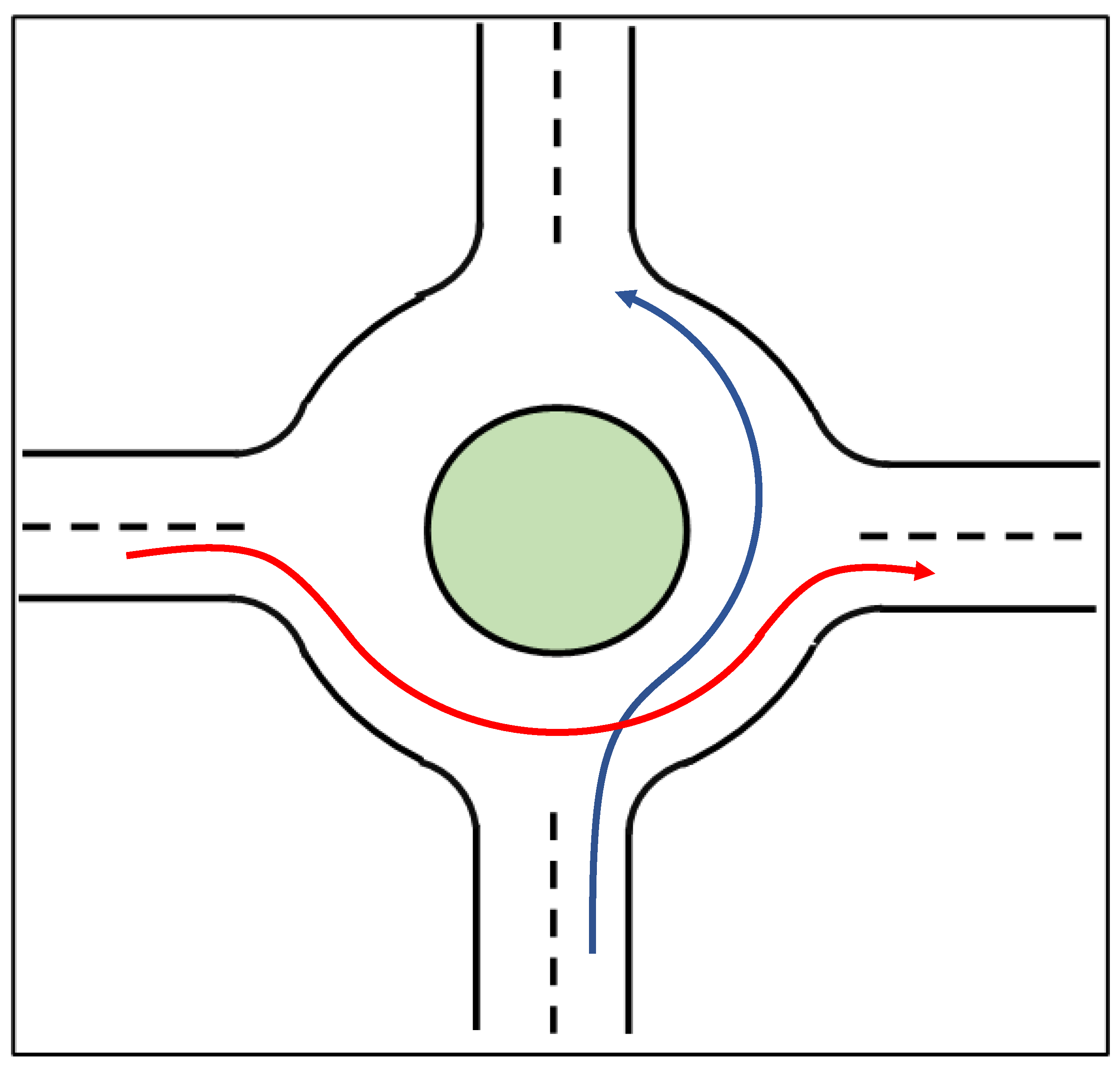
The goal of implementing the decision-making algorithm at a round intersection is to realize safe, comfortable and efficient driving of an autonomous vehicle that interacts with multiple other vehicles. To achieve this goal, not only is a decision-making algorithm necessary but good path planning is also required. However, path planning is out of the scope of this paper, and we will not discuss the path planning method here. The assumption made here is that the vehicle drives on a designated path through a round intersection, as illustrated in Figure 3, for two different vehicles. The blue line represents the path for the ego autonomous vehicle and the red line shows the path for another vehicle, which could be a human-driven vehicle or an autonomous vehicle. These two paths have an intersection point. Thus, to make sure that a collision does not happen at the intersection point between these two paths and that the ego vehicle can pass through the round intersection within a shorter time compared with executing a stop-wait-and-then-pass policy, a decision-making algorithm for a round intersection is necessary.
The vehicle model is an important factor for vehicle control in autonomous driving. Even though there is no perfect model to describe how the vehicle moves, there are several vehicle models commonly used since they show good approximations and performance for the vehicle control problem. An example is the single-track vehicle model [42]. Autonomous vehicle control can be modeled in a hierarchical architecture: high-level control for decision-making and low-level control for path following as well as the control for brake and throttle. In this paper, as we are mainly concentrating on the high-level decision-making part of vehicle control, a model that describes vehicle kinematic motion will be sufficient. Hence, we use the vehicle kinematic motion model in a discrete-time domain at a round intersection. The vehicle model for the ego vehicle with the subscript of r is given by
S t + 1 = T r ( S t , a t )
where S t represents the state vector of the vehicle and a t is the input to drive the model. Model (8) is expanded in detail as
x ( t + 1 ) = x ( t ) + v ( t ) cos θ ( t ) Δ t
y ( t + 1 ) = y ( t ) + v ( t ) sin θ ( t ) Δ t
v ( t + 1 ) = v ( t ) + a ( t ) Δ t
θ ( t + 1 ) = θ ( t ) + w ( t ) Δ t
In Equations (9)–(12), x ( t ) , y ( t ) describe the 2D planar position and θ ( t ) is the heading angle of the vehicle model with respect to a fixed coordinate system. v ( t ) is the linear velocity of the vehicle. The input a t that drives the vehicle is a ( t ) , w ( t ) , representing the linear acceleration and the angular velocity or the yaw rate of the vehicle. The acceleration determines how fast the vehicle can change its speed and direction. Δ t is the time step for the discrete model. In this paper, the above model is used for updating the states of the agent. Since the agent has no information on other vehicles, we assume that other vehicles will follow a similar model but with no speed or direction change given by
S t + 1 = T v ( S t )
which can be expanded as
x ( t + 1 ) = x ( t ) + v ( t ) cos θ ( t ) Δ t
y ( t + 1 ) = y ( t ) + v ( t ) sin θ ( t ) Δ t
v ( t + 1 ) = v ( t )
θ ( t + 1 ) = θ ( t )
The position information, the heading angle and the velocity of other vehicles will be collected each time a perception snapshot is made.
In this paper, the input of the ego vehicle is selected from a finite set of actions, { a 1 , a 2 , , a m } × { w 1 , w 2 , , w k } for linear acceleration and angular velocity. At every decision step, the ego vehicle will take a linear acceleration to determine its velocity and an angular velocity to determine its direction of driving. The change in the direction of the yaw rate introduces the discontinuity of tracking the vehicle motion using the model in Equation (8) and will influence the decision-making for the forward Monte-Carlo simulation part, which is discussed in detail later.
In this paper, without loss of generality, all road users are considered as vehicles driving on the road. Based on the vehicle models provided, the state space of all the objects contains the states of all the vehicles involved in the decision-making problem. For the decision-making cycle at time k , the state space is given by
S k = { s k e , s k 1 , , s k m }
The subscripts are the time stamps of the current decision-making cycle. The ego vehicle’s state is represented with superscript e , and superscripts 1 , , m are for the m other vehicles that are not controllable with the decision-making algorithm. s e = [ x , y , θ , v , w ] T . x , y , θ represent the longitudinal position, lateral position and yaw angle of the vehicle, respectively. These three values provide vehicle pose information. v , w are the linear velocity and yaw rate for describing the motion of the ego vehicle. For the other vehicles
s i = [ x , y , θ , v ] T ,   i = 1 , , m
where x , y , θ are the vehicle pose information and v is the linear velocity of the observed vehicle i. The difference in the state vector between the ego vehicle and other vehicles reveals partial observability in vehicle decision-making problems. Using the vehicle’s onboard sensors such as IMU, the ego vehicle can sense its yaw rate during driving. However, due to the limitation of sensors, the ego-vehicle will not be able to access other vehicles’ yaw rate values, hence the need to predict other vehicles’ future trajectories for planning and decision-making. The transition models are the vehicle models provided before. We assume that the state transitions are deterministic with a probability of transition given by
T : P ( s | s , a ) = 1
The observation states of the agent vehicle and the other vehicles are the same, with their state vector having an observation probability of 1. The uncertainty in perception and sensing is not discussed here and is out of the scope of this paper with
Z : P ( o | s , a ) = 1
Since the OOPOMDP method is used for the decision-making problem within a multi-vehicle round intersection traffic scenario, we also formalize the state space and observation space in the OOPOMDP fashion by noting the following:
  • C = { c r , c v } is the class of objects in the decision-making problem. In this problem, we consider two classes of objects, which are the ego vehicle class c r for the ego vehicle and the other vehicle class c v for other vehicles in the environment.
  • A t t ( C ) are the attributes of objects in different classes. The attributes of the ego vehicle class include the position information ( X , Y , θ ) and motion information ( v , w ) . The attributes of the other vehicle class include position information ( X , Y , θ ) and velocity v .
  • D o m ( a ) is the domain of attributes. The domain of attributes in this paper is mainly on the poses of vehicles. For both the ego vehicle class and the other vehicle class, the positional domain is within the area of the round intersection, and the heading angle is within the range of [ 0 , 2 π ) .
  • A is action set. The action is a combination of two finite set of actions, A = { a 1 , a 2 , , a m } × { w 1 , w 2 , , w k } for linear acceleration and angular velocity. Each action is selected from the set and results in a pair ( a i , w j ) ,   i = 1 m ,   j = 1 k .
The decision-making algorithm for a round intersection is based on the Partially Observable Markov Decision-Making Process, which can also be viewed as an optimization problem that optimizes the expected summary reward in the future horizon. Hence, a reward function or penalty function is required for awarding or penalizing the current action. In this paper, a penalty-style reward function is implemented. Wrong actions are penalized, which makes them a negative reward. The goal of the decision-making algorithm is to minimize the overall negative reward (penalization) of the agent traveling along the designated path through the round intersection, as given by
a * = arg max a A E [ t = 0 γ t R ( s t , a t ) | b 0 ]
The goal of this decision-making algorithm is to make sure that the agent can drive through the round intersection safely, efficiently and comfortably. The requirements for these three perspectives lead to the penalization of the risk of collision, the speed, the acceleration and the sound use of the road. The overall reward function for each step is given by
R ( s t , a t ) = c 1 R c o l l i s i o n ( s t , a t ) + c 2 R g a p ( s t , a t ) + c 3 R v e l o c i t y ( s t , a t ) + c 4 R t a r g e t ( s t , a t ) + c 5 R a c c ( s t , a t )
The reward in Equation (23) is made up of five different components. For the collision reward, the ego vehicle should not collide with other road users, as avoiding collisions and reducing traffic accidents is the top priority in designing any kind of decision-making algorithm. This reward is related to the nearest vehicle. Every time an action makes the ego vehicle get closer than some threshold safe distance to the nearest other vehicle, a large penalty given by
R c o l l i s i o n ( s t , a t ) = { 1000   if   d ( v e , v ) < = d s a f e 0   otherwise
is applied. In the above equation, d is the distance between the two vehicles given by
d ( v e , v ) = | x e x | 2 + | y e y | 2
which is the distance between the center of mass of the agent vehicle (ego vehicle) and that of the nearest vehicle of detection. d s a f e is determined by the dimensions of the vehicles and the speed limit of the road. As illustrated in Figure 4 below, to determine the safety bound of vehicles, a circular range around each vehicle is considered such that the boundary will not be influenced by the heading direction of vehicles. Therefore, the safety threshold distance is a summary of the threshold distance as well as the two radii of the circular boundaries generated from the vehicles’ dimensions and is given by
d s a f e = d t h r e s h o l d + R e , b o u n d a r y + R b o u n d a r y
d t h r e s h o l d = v lim 2 2 a max
R e , b o u n d a r y = W e 2 + ( L e / 2 ) 2 , R b o u n d a r y = W 2 + ( L / 2 ) 2
In Equations (26)–(28), v lim is the speed limit on a given road segment, a m a x is the maximum allowed deceleration of a vehicle for which the passengers in the vehicle will not feel uncomfortable and d t h r e s h o l d shows the emergency distance when the ego vehicle (the blue vehicle in the back) needs to make an emergency brake to fully stop in order to avoid a collision with the front vehicle (the orange vehicle). W represents the width of the vehicles. L is the length of the vehicles. Equation (27) uses a worst-case stopping distance analysis and, hence, uses the largest allowable speed vlim. If a less conservative result is desired, the current speed of the ego vehicle can be used instead.
The ego vehicle is penalized for its speed being lower than the speed limit of the current road segment because the vehicle is always expected to drive at the limit speed of the current road segment for efficiency. It is also penalized if it exceeds the speed limit. The penalty for exceeding the speed limit is larger than being lower than the limit speed. The penalty for discomfort is, then, introduced as
R v e l o c i t y = { C e x c e e d | v e v d e s | v d e s   if   v e > v d e s C l o w e r | v e v d e s | v d e s   if   v e < v d e s
where C e x c e e d and C l o w e r are negative constant coefficients for the situation where the ego velocity v e is larger than or smaller than the desired velocity v d e s , respectively. The desired velocity is determined according to the largest tolerance to lateral acceleration for passengers in the vehicle if the vehicle is turning and follows the road speed limitation if the vehicle is traveling on a straight road as
v d e s = { a y , max / κ   if   turning v l i m i t   otherwise
where κ in Equation (30) is the radius of curvature while turning. The velocity reward drives the ego vehicle toward the desired velocity if there is no risk of collision with the other vehicles. If there is a chance of collision, the velocity reward is dominated by the penalty caused by the collision risk due to the difference in scales between these two rewards. Regarding the comfort of the passengers in the vehicle, the maximum acceleration is limited as
a = a x 2 + a y 2 < = a max .
Therefore, once the overall acceleration is larger than a max , a penalty for discomfort is introduced in the reward function for causing discomfort to the passengers in the vehicle. The longitudinal acceleration part a x is the currently selected action from the action set. The lateral acceleration a y is derived from the lateral motion of the vehicle as
a y = v 2 / r = v 2 κ
Since the vehicle is following a designated path, the target area is also pre-determined on the path. Once the vehicle is within the target point of the path, it will be rewarded. The negative reward (cost), given by
R a c c = { 100   if   a a m a x 0     otherwise
is used to penalize acceleration above the threshold amax. Braking deceleration limiting was used here as acceleration was readily available. It should be noted that jerk can also be used in the reward function as an alternative.
Apart from the commonly used reward settings, as can be seen in other works, a gap reward is also proposed for driving efficiency on the road in the decision-making algorithm in this paper. Intersections, especially round ones, are the most crowded traffic scenarios in urban traffic with vehicles merging from different road segments. In addition to the requirement of safety, efficient use of the road space is also necessary to reduce the chance of a traffic jam. The gap reward aims to drive the agent vehicles to follow the proceeding vehicle at a certain distance. A commonly accepted 3 s rule for vehicle following is used to generate the desired gap between the agent vehicle and the preceding vehicle as
v 3 s = max { v e 3 b max , 0 }
d d e s i r e d = v e 2 v 3 s 2 2 a max
R g a p = c g a p | d ( v e , v ) d d e s i r e d |
In Equation (34), v 3 s is the target velocity when acting an emergency full brake at the maximum brake acceleration b max and d d e s i r e d is the preferred gap between the ego vehicle and the nearest preceding vehicle. A negative reward Rgap is assigned according to Equation (36) if the distance is different from the desired gap between vehicles. It should be noted that there is a tradeoff between safety (Rcollision) and the efficiency of travel (Rgap), which are conflicting goals.

4. Improving Decision-Making with Policy Prediction

Decision-making and planning for autonomous vehicles in urban traffic scenarios has always been a challenging problem due to the complexity of urban traffic. Another challenge is the tracking of vehicle driving motion in the urban area, which largely influences the performance of the decision-making algorithm. There are several research works that have been conducted to improve the vehicle planning algorithm’s performance. Ref. [42] proposed the method of adjusting the vehicle model parameters (Intelligent Driver Model or IDM model parameters) to emulate different styles of driving and tried to improve the decision-making algorithm for highway autonomous driving performance. Ref. [43] proposed a game-theoretic planning algorithm for all vehicles in the traffic scenario in round intersections. Ref. [44] proposed a method that uses a hidden mode stochastic hybrid system to model different human driving behaviors to assist the performance of decision-making in a driver assistance system. Yet, there are few works on improving the autonomous vehicle decision-making problem for round intersections with multiple vehicles involved. Hence, in this section, a policy-prediction method-based improvement for autonomous vehicle decision-making is proposed as one of the main contributions of this paper.
The planning and decision-making problem can be regarded as a receding horizon optimization problem starting from the current time and extending to a future time based on the horizon of the optimization problem. The ego vehicle obtains an observation of all the other surrounding vehicles at time t, noted as o t , and tries to find an optimal action such that the total reward is maximized as
a * = arg max a A E [ t = t t + k γ t R ( s t , a t ) ] .
We do not have full knowledge of all the future states along the planning horizon. It is essential to have a good prediction over the future state trajectories, and the state transition model needs to have good precision for tracking the future potential trajectories.
For the decision-making and planning of autonomous vehicles, the vehicle trajectory tracking over a future horizon can be performed with the state transition model as described in Equations (13)–(17). For highways, it is rather simple since the vehicles tend to not have rough behaviors like multiple lane-changing within a short time, for example. The model in Equation (13) can provide good trajectory tracking for the decision-making problem on a highway. The case is different for planning in the urban traffic environment for intersections, especially round intersections. The vehicle needs to change the direction of driving in a short period of time due to the geometric features of intersections. The current observations of other vehicles do not provide enough information on how they will move in the future time horizon for planning.
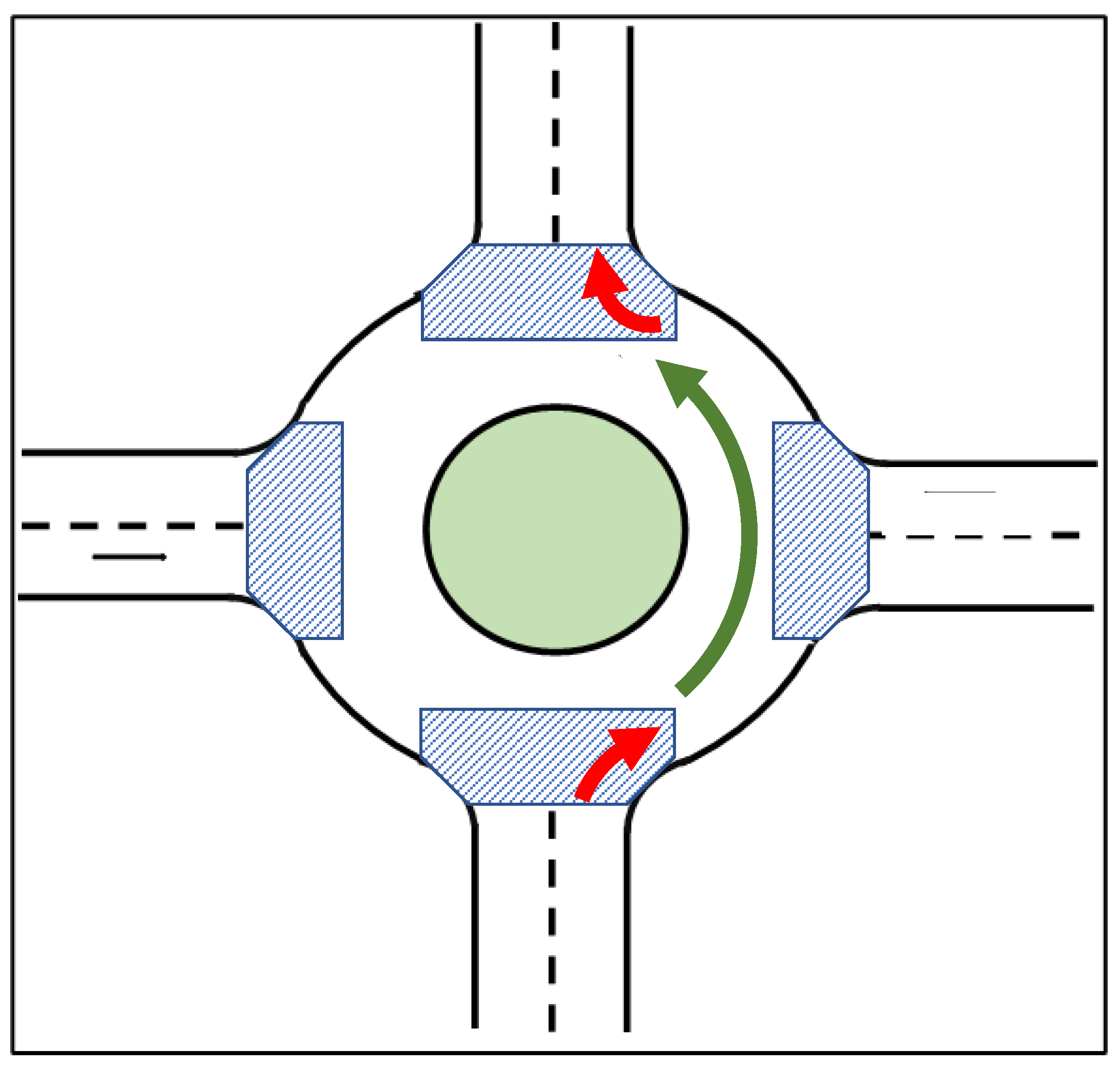
As a demonstrative example, the path of a vehicle passing a round intersection is shown in Figure 5. The shadowed areas in the figure are the areas in which a vehicle is entering or exiting the round intersection. The vehicle first travels through a shadowed area to enter the round intersection and makes a turn in a clockwise direction, as shown by the bottom red arrow. After passing the shadowed area to enter the round intersection, the vehicle follows the lane area and takes a constant yaw angle turning in the counterclockwise direction, as shown by the green arrow. Reaching the target connection point to exit, the vehicle now makes a clockwise turn to exit the round intersection and drive on the straight road again, as shown by the red arrow on the top. Throughout the whole procedure of passing the round intersection, the vehicle shows a discontinuous motion in the driving direction, and the yaw rate keeps changing along the path, making it hard for the vehicle motion model (10) to track given a single initial condition.
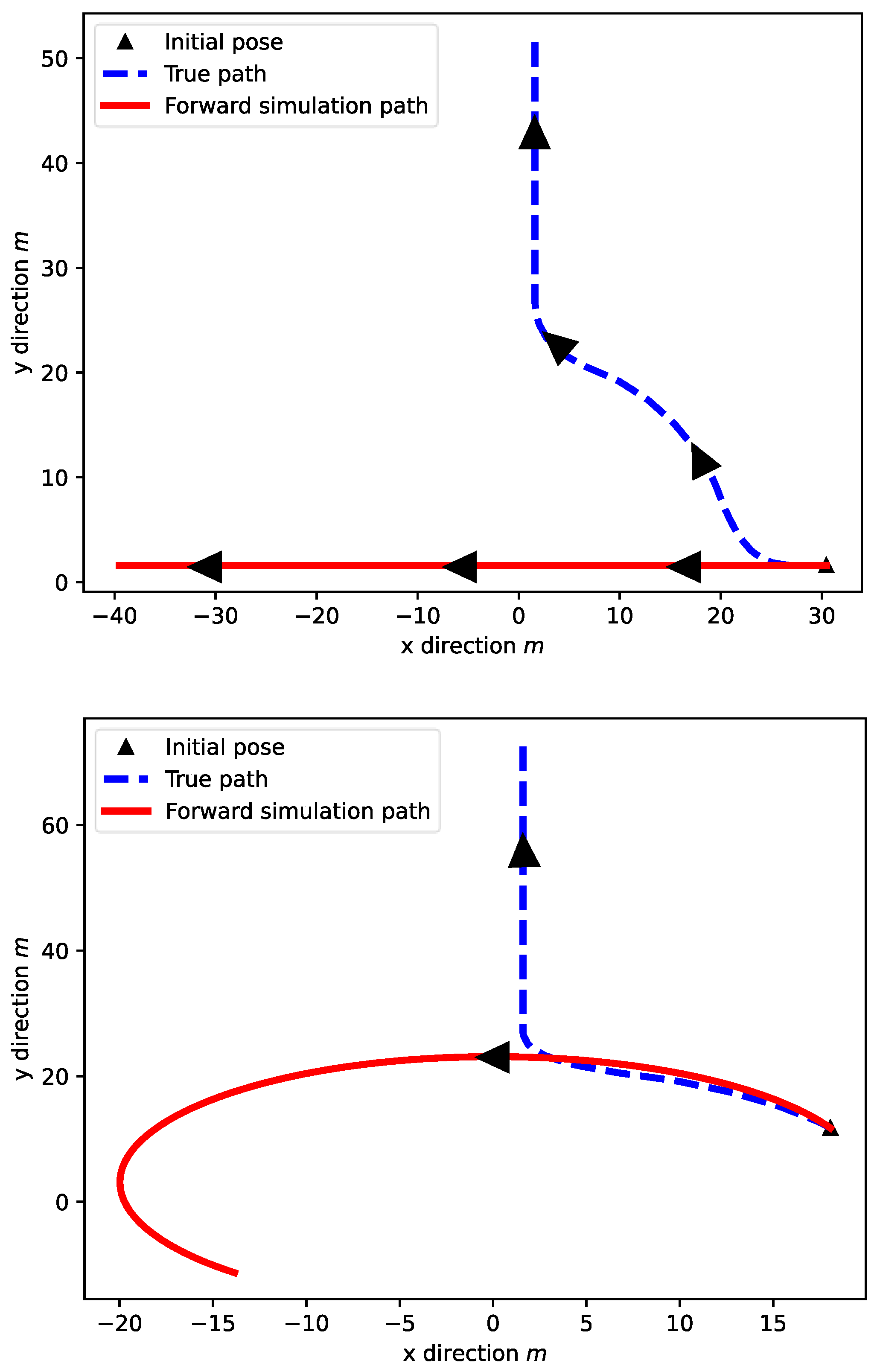
In a decision-making cycle, the planning starts from some initial state sampled from the belief state space at current time, denoted as t 0 , and carries out a forward simulation to generate potential trajectories of the states for optimizing the expected cumulative reward along the optimization horizon t 0 ~ t 0 + k , with k being the decision-making horizon. Directly implementing the vehicle motion models in Equation (10), even with the knowledge of the yaw rate at t 0 , the true trajectory deviates a lot from the simulated trajectory that tracks the potential vehicle trajectory on the optimization horizon. The model alone is not enough to describe the vehicle state transitions under the round intersection traffic scenarios, as shown in Figure 6. In Figure 6, the true trajectories are not successfully tracked by directly implementing the state transition equations from the initial state. The forward simulation path is calculated for 100 steps, and the arrows show the direction of the vehicle moving or the direction of the simulation. This will cause a lot of issues when making decisions for the ego vehicle to pass the round intersection safely and efficiently. This issue will also affect the solution of the POMDP problem based on the Monte-Carlo Tree search since the Monte-Carlo simulation for the state particles is the core procedure in the tree search algorithm.
To overcome the issue caused by the discontinuity in vehicle motion, a policy-prediction-based decision-making method is proposed here, such that the state transition of the vehicle can be better tracked and simulated during the decision-making cycle. The policy-prediction method is based on the change point policy-prediction method. This paper mainly focuses on the traffic scenario of round intersections, and an abstract policy set is applied here for the decision-making algorithm. This method utilizes the recorded history of the decision-making algorithm based on the OOPOMDP so that it avoids additional memory costs.

5. Augmented Objective State and Policy-Based State Transition

The original setting of the observation state is the same as the state of the other vehicles, that is
s t i = o t i = [ x i , y i , θ i , v i ] T
where the observation state o t i is the real observation made by the agent from the environment. It does not contain any of the policy information, so the states sampled from the updated belief states directly accomplish state transition using the model (10) during the decision cycle. This leads to the issue of the simulated path deviating from the true path and causing inaccuracy in decision-making. Here, an attribute is added to the other vehicle class c v for the most recent policy π i that augments the state space and observation space into
s t , a i = o t , a i = [ x i , y i , θ i , v i , π i ] T
where π i is the most likely policy that the observed vehicle is executing at the time that current observation is made for vehicle i. We denote the policy prediction method as
F : h π t i , i { 1 , 2 , , n }
where h is the current history of the POMDP problem, and, as shown in a previous section, it is a series of actions and observations made by the agent and given by
h t = { b 0 , a 0 , o 1 , a 1 , o 2 , , a t 1 , o t } .
According to the feature of the OOPOMDP, the observations of other vehicles can also be indexed by objects in the history. So, we can use it for policy-prediction methods for each of the vehicles involved in the traffic scenario. π t i Π is a policy for vehicle i selected from the pre-determined policy set. For every decision cycle, we first obtain the history of observations on vehicle i and implement the policy-prediction method to find the policy over the last segment of the vehicle and then augment the observations state and state of vehicle i with the potential policy so that the policy can be used for state transitions during the Monte-Carlo Tree search. The state transition equation of other vehicles is now modeled as
S t + 1 = T v ( S t , π t )
with
x ( t + 1 ) = x ( t ) + v ( t ) cos θ ( t ) Δ t
y ( t + 1 ) = y ( t ) + v ( t ) sin θ ( t ) Δ t
v ( t + 1 ) = v ( t )
θ ( t + 1 ) = θ ( t ) + w ( π i , θ ^ π i ) d t
Vehicle model (13) now becomes a constant velocity and turn rate model for vehicle trajectory tracking. The yaw rate is generated based on the current policy π i and parameter θ ^ π i , which will help with vehicle trajectory tracking in the decision-making cycle and improve the performance of decision-making based on the OOPOMCP algorithm.
Since the decision-making algorithm is mainly used for vehicles traversing a round intersection, we take advantage of its geometry to simplify the generation procedure of the vehicle yaw rate based on the policy. According to the geometric features of a round intersection, we know that a round intersection has mainly three types of areas: straight road segments, enter/exit areas and round areas. The vehicle yaw rate will also be determined by road curvatures in these three different types of areas based on
w = v / r = v κ
where r is the turning radius of the vehicle trajectory and κ is the road curvature.
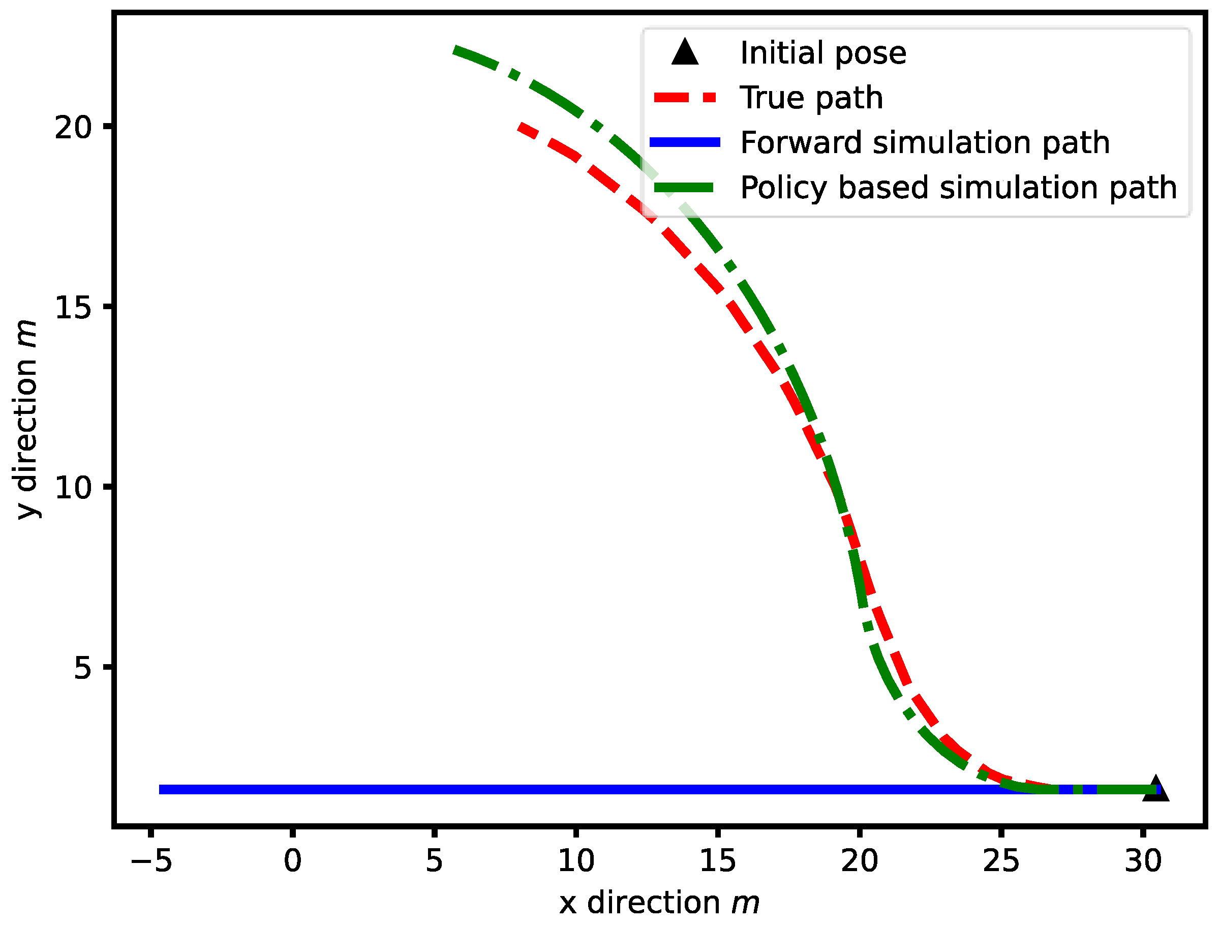
To illustrate the difference in utilizing this method, a forward simulation trajectory is generated with the policy-based state transition model, as shown Figure 7. From Figure 7, we can see that the policy-based simulated path is very similar to the true path of a vehicle passing a round intersection, where only the initial state is given. In the simulated path generation, we assume that the policy of entering the round intersection is given such that the vehicle yaw rate is generated based on the policy, so the vehicle is turning in a clockwise direction to enter the round intersection instead of keeping the original heading angles and yaw rate from the straight lane. In this case, the decision made by the agent vehicle will be closer to the real situation and improve the performance of the decision-making algorithm.
In addition to using the policy-based state transition in the decision-making problem of vehicles in a round intersection, the control of the autonomous vehicle also considers vehicle jerk. Since the reward function can measure how good it is for the current selection of an action from the action set, it is able to measure the rewards caused by a velocity that exceeds the speed limit or exceeds the maximum lateral acceleration that causes discomfort. However, it is not capable of measuring the change in acceleration (jerk) since the reward function does not have access to previous actions. Therefore, the previous linear acceleration is stored for comparison with current acceleration determined with the tree search. We approximate the jerk of the vehicle to be given by
J t = | Δ a | = | a t a t 1 |
Based on this jerk indication J t , an acceleration re-selection is made to ascertain that the acceleration change does not exceed a maximum allowed jerk so that the vehicle speed change is smooth and passengers feel comfortable. This is based on
a t = { a t if   J t < = J max a t 1 + J m a x if   a t a t 1 > = J max a t 1 J m a x   if   a t a t 1 < = J max
which is used to make sure that the jerk of the autonomous vehicle is not too large.

6. Results and Discussion

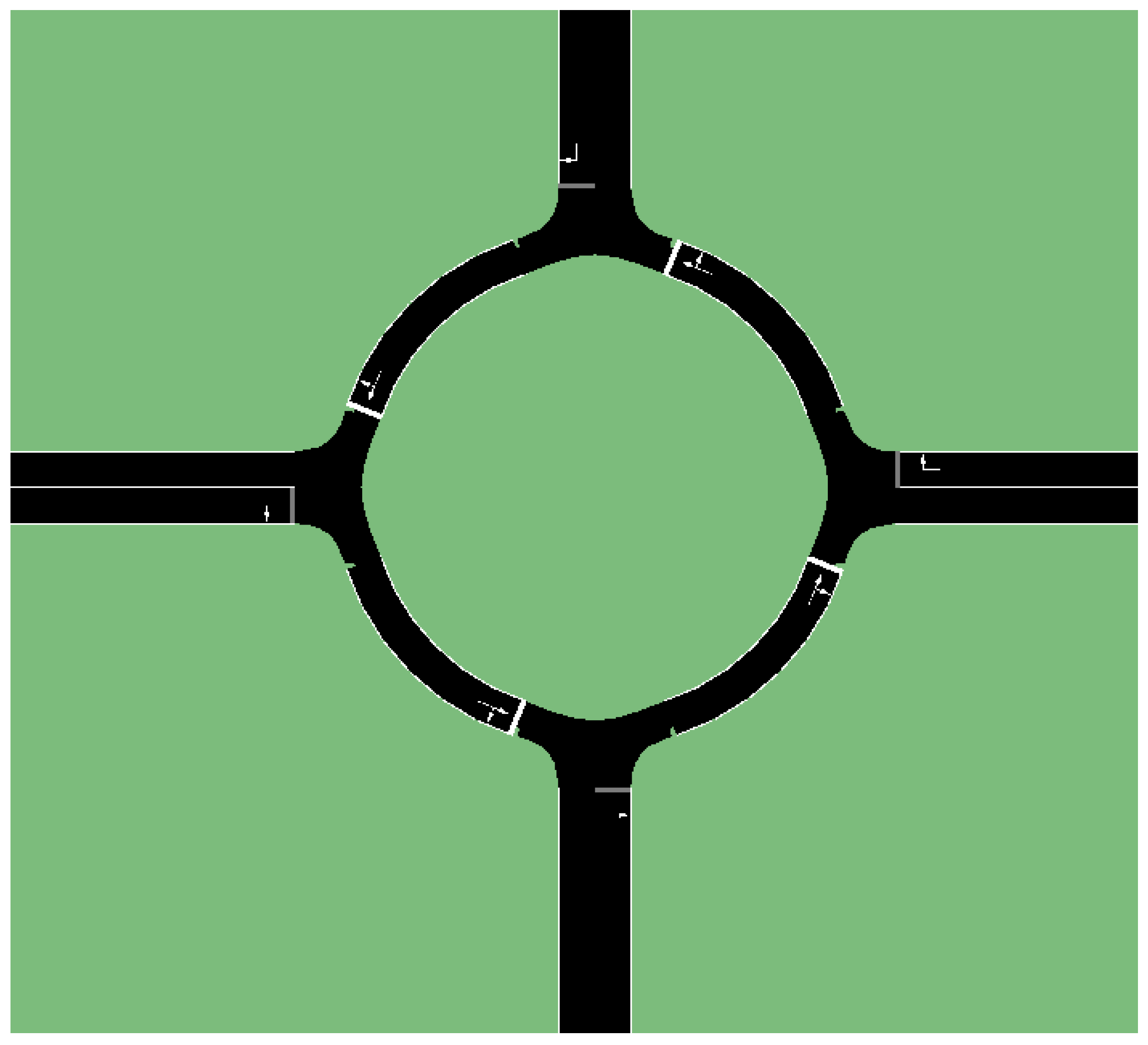
The simulation of decision-making for autonomous vehicles passing a round intersection is carried out, and exemplary results are summarized here to test and validate the decision-making algorithm with a policy-based state transition. The traffic scenario in the simulation is a typical four-way round intersection, as shown in Figure 8. Vehicles enter the scenario from the straight lane segment and move toward their destination area. To simplify the test environment, we assume the round intersection is a circle so that the road curvature within the round intersection is a constant: κ = 1 / r , where r is the radius of curvature of the lanes in the round intersection. During the simulation, vehicles drive on the right side of the road on the straight lane segment and in the counterclockwise direction while they are within the round intersection.
For the OOPOMCP algorithm to solve the Object-Oriented POMDP problem, the parameters used in the tree search are:
  • Planning time for each step: 1.0 s;
  • Maximum search depth in the tree: 100;
  • Exploration constant value: 2.0;
  • Discount factor of the cumulative expected reward: 0.99.
In the action set, the discrete linear acceleration set given by
A c c = { 3.0 , 2.0 , 1.0 ,   0 ,   0.5 ,   1.5 ,   2.5 }   m / s 2
is used. The yaw rate of the vehicle can be determined according to the road curvature using the linear velocity at different road segments for the round intersection. As for a single-lane round intersection with a straight road segment connecting to it, the yaw rate appears to have three features:
  • In the straight lane segments, the vehicle’s yaw rate is maintained at zero as it keeps driving straight.
  • In the round intersection part, the vehicle drives along the road at the yaw rate of w = v R , where R is the radius of the round intersection and v is the vehicle’s linear velocity. This is a positive value when setting the counterclockwise direction as the positive direction.
  • When the vehicle is entering/exiting the round intersection, the yaw rate w is some negative value when the counterclockwise direction is taken as the positive direction. In the simulation, since the entering/exiting process only takes a very short time period, the yaw angle change is approximated with a yaw rate determined by the process of uncontrolled simulation vehicles entering the round intersection.
In the simulation, the round intersection has a radius curvature of 20 m; hence, the road curvature in the roundabout intersection is 1/20. Additionally, based on the test data, the curvature of the entering/exiting area in the simulation is approximated to be 0.15, which is used in the transition model. Apart from those parameters in the action set, parameters for the reward function in the decision-making problem are listed below. Currently, all the factors in the total reward are equally weighted; hence, the coefficients used are
c 1 = c 2 = c 3 = c 4 = c 5 = 1 .
The collision reward depends on the vehicle dimensions. In this test, the vehicles have the same dimension, which are L = 5.0   m , W = 1.8   m . These are the default settings of the passenger vehicles in the SUMO simulation.
The overall maximum acceleration required in Equation (33) is set to be 4.0 m / s 2 , and the maximum lateral acceleration caused by vehicle turning is set to be 2.0 m / s 2 . The cost due to exceeding the desired velocity in Equation (29) is C e x c e e d = 100 for penalizing the unsafe maneuvering of exceeding the maximum allowed velocity, and the cost for being lower than the desired velocity is C l o w e r = 10 . The maximum brake acceleration is the lowest acceleration from the action set, which is −3.0 m / s 2 and c g a p = 10 .
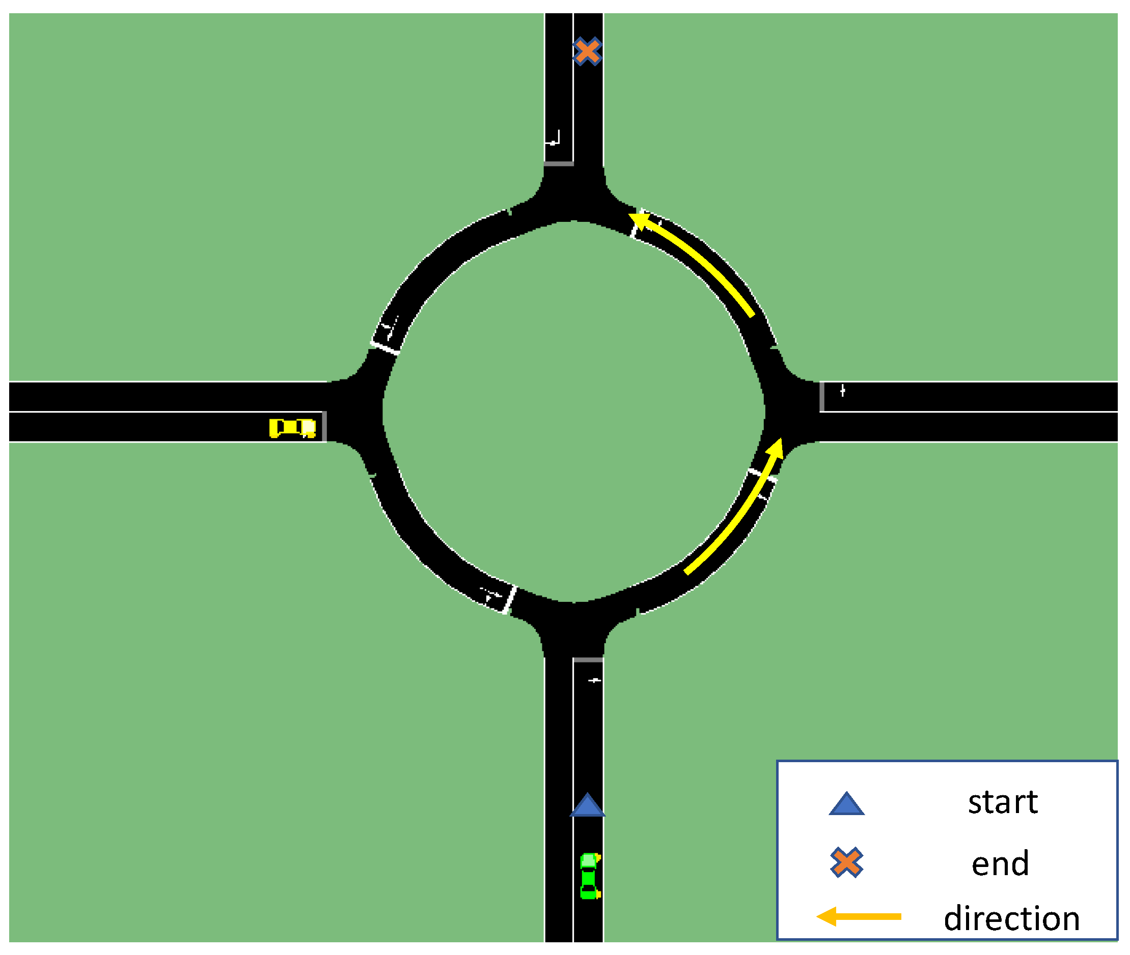
The simulation results compare the performance of the decision-making algorithm with decision-making using the OOPOMDP with and without a policy-based state transition against the benchmarking system of the SUMO simulation system built-in vehicle model, which is an Intelligent Driver Model (IDM) that executes lane following. The results compare the total travel time, total reward and if there is an emergency brake acted by other vehicles in the system. First, a two-vehicle scenario simulation is performed, and the results are presented below. The diagram of the two-vehicle scenario is presented in Figure 9. The autonomous vehicle, colored green, traverses the round intersection starting from the bottom and tries to reach the destination points at the top in the figure. The simulation results for this two-vehicle scenario are summarized in Table 1.
From the results above in Table 1, we can find that the OOPOMDP with the policy-based state transition method proposed in this paper achieves a higher reward (less negative) compared with the one that directly implements the state transition model proposed in Equation (13). With the policy-based state transition, the ego vehicle can better predict the future trajectory of the surrounding vehicles and control the speed and direction to reach its destination in a shorter time. Also, since it avoids the risk of colliding with other vehicles, no emergency brakes or aggressive maneuvers need to be made by other vehicles while they are following the lane with their IDM models. Also, the shorter time achieved when compared with the system driver proves the efficiency of implementing such a decision-making algorithm for autonomous vehicles in round intersections.
Another simulation is carried out for a multi-vehicle scenario. Eight vehicles in total are involved in the simulation with different departure times. Hence, they interact within the region of the round intersection, as shown in Figure 10. The green vehicle shows the ego vehicle that deploys the decision-making algorithm, and the test results are summarized in Table 2.
In this simulation, whose results are summarized in Table 2, decision-making with the policy-based state transition is able to achieve the goal of traversing the round intersection safely and efficiently without any potential collision, and it takes advantage of road space to drive fast. Yet, we see that the OOPOMDP-based decision-making has a large penalty (negative total reward) because a potential collision that generates a very large penalty happens due to the inaccuracy in predicting other vehicles’ trajectories, as shown in Figure 11. The long traversal time of the system driver is due to the right-of-way. The ego vehicle has to wait for other vehicles to pass in the round intersection. Thus, the waiting time is very long compared with the result of implementing the POMDP decision-making algorithms in this paper.
The experimental results for the two cases considered were presented in this section with illustrations and in the form of Table 1 and Table 2, which summarize the results. This paper focused on the decision-making problem of being able to handle a round intersection without any collisions, and the results were presented accordingly. The path of the AV was pre-determined for this reason.

7. Conclusions and Recommendations

In this paper, methods for decision-making and planning of autonomous vehicles in handling a round intersection were introduced and discussed along with simulation results for the validation of the algorithms. The POMDP was first introduced as a powerful tool for solving the sequential decision-making problem with uncertainties and states that are not fully observable. The OOPOMDP algorithm was later introduced as a method for factoring object states and observations individually and making the belief update more efficient and low-cost. Utilizing the feature of the OOPOMDP, a policy-based state transition was used for the decision-making algorithm. Since the OOPOMDP stores the history of all the involved agents and environment objects, the agent gets to determine the most recent policy of other vehicles based on the policy-prediction method that was introduced. This OOPOMDP decision-making with policy prediction largely improves the performance of decision-making for the traffic scenario of round intersections. The reward function was formulated for safe and efficient travel while keeping passenger comfort in mind.
The approach in this paper can be applied to other relevant connected and autonomous driving tasks. For example, the platooning or convoying of vehicles in the form of adaptive and cooperative adaptive cruise control [45,46] on highways is a topic with much research attention. More recent work focuses on similar cooperative driving in urban roads including cooperative handling of an intersection by a convoy of cooperating vehicles [47]. While there are results for straight intersections, corresponding results for round intersections are missing. The approach in this paper can be useful for the cooperative handling of round intersections by a convoy of connected and autonomous vehicles. Active safety control systems like yaw stability controllers [48] are also important as the vehicles in the round intersections follow a circular path and yaw stability problems may occur due to weather conditions or emergency maneuvers. An extension of the approach in this paper can incorporate a more detailed model of the ego vehicle and can be integrated with yaw stability control to accommodate such problems.
It should be noted that the current paper only treats one round intersection as the focus is on the decision-making of one AV as opposed to the effect of the proposed decision-making algorithm on how multiple AVs with the decision-making algorithm would perform in a large traffic network. Simulations on a large road network considering different penetration rates of AVs using the proposed decision-making algorithm can be part of a future study. Similarly, work on how the results can be used for practical policy implications in various geographic jurisdictions worldwide was not considered here and can be part of future work.
The use of real-time data and a real-world implementation would be very useful as simulation is typically based on several unrealistic assumptions, and the traffic encountered in the field exhibit stochastic, dynamic and intricate characteristics. It is not possible for us legally to operate autonomously on public roads, so it was not possible for us to try this method in a real round intersection. Playback of real data in the simulations would also not be very realistic, as the data for other traffic would not be reactive to our ego AV. As a result, we used SUMO simulations in this paper. Future work can implement this decision-making algorithm in real round intersections in controlled environments.

Author Contributions

Conceptualization, X.L., L.G. and B.A.-G.; methodology, X.L. and L.G.; software, X.L.; validation, X.L.; formal analysis, X.L.; investigation, X.L.; resources, L.G. and B.A.-G.; data curation, X.L.; writing—original draft preparation, X.L.; writing—review and editing, L.G. and B.A.-G.; visualization, X.L.; supervision, L.G.; project administration, L.G. and B.A.-G.; funding acquisition, L.G. and B.A.-G. All authors have read and agreed to the published version of the manuscript.

Funding

The authors acknowledge partial support from the Smart Campus organization (21824) of Ohio State University in support of the Smart Columbus project.

Data Availability Statement

Data are contained within the article.

Acknowledgments

The authors thank the support of the Automated Driving Lab at the Ohio State University.

Conflicts of Interest

The authors declare no conflict of interest.

References

  1. Gkartzonikas, C.; Gkritza, K. What have we learned? A review of stated preference and choice studies on autonomous vehicles. Transp. Res. Part C 2019, 98, 323–337. [Google Scholar] [CrossRef]
  2. Rana, M.M.; Hossain, K. Connected and Autonomous Vehicles and Infrastructures: A Literature Review. Int. J. Pavement Res. Technol. 2023, 16, 264–284. [Google Scholar] [CrossRef]
  3. Reyes-Muñoz, A.; Guerrero-Ibáñez, J. Vulnerable Road Users and Connected Autonomous Vehicles Interaction: A Survey. Sensors 2022, 22, 4614. [Google Scholar] [CrossRef] [PubMed]
  4. Sadid, H.; Antoniou, C. Modelling and simulation of (connected) autonomous vehicles longitudinal driving behavior: A state-of-the-art. IET Intell. Transp. Syst. 2023, 17, 1051–1071. [Google Scholar] [CrossRef]
  5. Guvenc, L.; Guvenc, B.A.; Emirler, M.T. Connected and Autonomous Vehicles. In Internet of Things and Data Analytics Handbook; John Wiley & Sons, Ltd.: Hoboken, NJ, USA, 2017; pp. 581–595. ISBN 978-1-119-17360-1. [Google Scholar]
  6. Claussmann, L.; Revilloud, M.; Gruyer, D.; Glaser, S. A Review of Motion Planning for Highway Autonomous Driving. IEEE Trans. Intell. Transp. Syst. 2020, 21, 1826–1848. [Google Scholar] [CrossRef]
  7. Kuwata, Y.; Teo, J.; Fiore, G.; Karaman, S.; Frazzoli, E.; How, J.P. Real-Time Motion Planning with Applications to Autonomous Urban Driving. IEEE Trans. Control Syst. Technol. 2009, 17, 1105–1118. [Google Scholar] [CrossRef]
  8. Yurtsever, E.; Lambert, J.; Carballo, A.; Takeda, K. A Survey of Autonomous Driving: Common Practices and Emerging Technologies. IEEE Access 2020, 8, 58443–58469. [Google Scholar] [CrossRef]
  9. Kuutti, S.; Fallah, S.; Katsaros, K.; Dianati, M.; Mccullough, F.; Mouzakitis, A. A Survey of the State-of-the-Art Localization Techniques and Their Potentials for Autonomous Vehicle Applications. IEEE Internet Things J. 2018, 5, 829–846. [Google Scholar] [CrossRef]
  10. Guvenç, L.; Guvenç, B.A.; Demirel, B.; Emirler, M.T. Control of Mechatronic Systems; IET Control, Robotics and Sensors Series; The Institute of Engineering and Technology: London, UK, 2017; ISBN 978-1-78561-145-2. [Google Scholar]
  11. Guvenc, L.; Aksun-Guvenc, B.; Zhu, S.; Gelbal, S.Y. Autonomous Road Vehicle Path Planning and Tracking Control; Book Series on Control Systems Theory and Application; Wiley/IEEE Press: New York, NY, USA, 2021; ISBN 978-1-119-74794-9. [Google Scholar]
  12. Li, S.; Shu, K.; Chen, C.; Cao, D. Planning and Decision-making for Connected Autonomous Vehicles at Road Intersections: A Review. Chin. J. Mech. Eng. 2021, 34, 133. [Google Scholar] [CrossRef]
  13. Schwarting, W.; Alonso-Mora, J.; Rus, D. Planning and Decision-Making for Autonomous Vehicles. Annu. Rev. Control Robot. Auton. Syst. 2018, 1, 187–210. [Google Scholar] [CrossRef]
  14. Gelbal, S.Y.; Aksun-Guvenc, B.; Guvenc, L. SmartShuttle: A Unified, Scalable and Replicable Approach to Connected and Automated Driving in a Smart City. In Proceedings of the Science of Smart City Operations and Platforms Engineering in partnership with Global City Teams Challenge (SCOPE-GCTC) Workshop, Pittsburgh, PA, USA, 18–21 April 2017. [Google Scholar]
  15. Al-Turki, M.; Ratrout, N.T.; Rahman, S.M.; Assi, K.J. Signalized Intersection Control in Mixed Autonomous and Regular Vehicles Traffic Environment—A Critical Review Focusing on Future Control. IEEE Access 2022, 10, 16942–16951. [Google Scholar] [CrossRef]
  16. Li, X.; Zhu, S.; Aksun-Guvenc, B.; Guvenc, L. Development and Evaluation of Path and Speed Profile Planning and Tracking Control for an Autonomous Shuttle Using a Realistic, Virtual Simulation Environment. J. Intell. Robot. Syst. 2021, 101, 42. [Google Scholar] [CrossRef]
  17. Savolainen, P.T.; Gates, T.J.; Gupta, N.; Megat-Johari, M.U.; Cai, Q.; Imosemi, S.; Ceifetz, A.; McArthur, A.; Hagel, E.C.; Smaglik, E.J. Evaluating the Performance and Safety Effectiveness of Roundabouts–An Update; Report Number: SPR-1725; Michigan Department of Transportation: Grand Rapids, MI, USA, 2023. [Google Scholar]
  18. Elvik, R. Road safety effects of roundabouts: A meta-analysis. Accid. Anal. Prev. 2017, 99, 364–371. [Google Scholar] [CrossRef] [PubMed]
  19. Wang, W.; Jiang, L.; Lin, S.; Fang, H.; Meng, Q. Imitation learning based decision-making for autonomous vehicle control at traffic roundabouts. Multimed. Tools Appl. 2022, 81, 39873–39889. [Google Scholar] [CrossRef]
  20. Monsalve, B.; Aliane, N.; Puertas, E.; Andrés, J.F. Think Aloud Protocol and Decision Tree for Driver Behavior Modeling at Roundabouts. IEEE Access 2023, 11, 41444–41454. [Google Scholar] [CrossRef]
  21. Sana, F.; Azad, N.L.; Raahemifar, K. Autonomous Vehicle Decision-Making and Control in Complex and Unconventional Scenarios—A Review. Machines 2023, 11, 676. [Google Scholar] [CrossRef]
  22. Muffert, M.; Pfeiffer, D.; Franke, U. A Stereo-Vision Based Object Tracking Approach at Roundabouts. IEEE Intell. Transp. Syst. Mag. 2013, 5, 22–32. [Google Scholar] [CrossRef]
  23. Okumura, B.; James, M.R.; Kanzawa, Y.; Derry, M.; Sakai, K.; Nishi, T.; Prokhorov, D. Challenges in Perception and Decision Making for Intelligent Automotive Vehicles: A Case Study. IEEE Trans. Intell. Veh. 2016, 1, 20–32. [Google Scholar] [CrossRef]
  24. Banjanovic-Mehmedovic, L.; Halilovic, E.; Bosankic, I.; Kantardzic, M.; Kasapovic, S. Autonomous Vehicle-to-Vehicle (V2V) Decision Making in Roundabout using Game Theory. Int. J. Adv. Comput. Sci. Appl. 2016, 7, 292. [Google Scholar] [CrossRef]
  25. Shen, M.; Sun, J.; Zhao, D. The Impact of Road Configuration in V2V-Based Cooperative Localization: Mathematical Analysis and Real-World Evaluation. IEEE Trans. Intell. Transp. Syst. 2018, 19, 3220–3229. [Google Scholar] [CrossRef]
  26. Fitzpatrick, C.D.; Abrams, D.S.; Tang, Y.; Knodler, M.A. Spatial and Temporal Analysis of Driver Gap Acceptance Behavior at Modern Roundabouts. Transp. Res. Rec. 2013, 2388, 14–20. [Google Scholar] [CrossRef]
  27. Wang, Z.; Liu, X.; Wu, Z. Design of Unsignalized Roundabouts Driving Policy of Autonomous Vehicles Using Deep Reinforcement Learning. World Electr. Veh. J. 2023, 14, 52. [Google Scholar] [CrossRef]
  28. Hang, P.; Huang, C.; Hu, Z.; Xing, Y.; Lv, C. Decision Making of Connected Automated Vehicles at an Unsignalized Roundabout Considering Personalized Driving Behaviours. IEEE Trans. Veh. Technol. 2021, 70, 4051–4064. [Google Scholar] [CrossRef]
  29. Farkas, Z.; Mihály, A.; Gáspár, P. Model Predictive Control Method for Autonomous Vehicles in Roundabouts. Machines 2023, 11, 75. [Google Scholar] [CrossRef]
  30. Cao, H.; Zoldy, M. MPC Tracking Controller Parameters Impacts in Roundabouts. Mathematics 2021, 9, 1394. [Google Scholar] [CrossRef]
  31. Ozcan, D.; Sonmez, U.; Guvenc, L. Optimisation of the Nonlinear Suspension Characteristics of a Light Commercial Vehicle. Int. J. Veh. Technol. 2013, 2013, 562424. [Google Scholar]
  32. Klos, M.J.; Sobota, A. Performance evaluation of roundabouts using a microscopic simulation model. Sci. J. Silesian Univ. Technology. Ser. Transp. 2019, 104, 57–67. [Google Scholar] [CrossRef]
  33. Arroju, R.; Gaddam, H.K.; Vanumu, L.D.; Rao, K.R. Comparative evaluation of roundabout capacities under heterogeneous traffic conditions. J. Mod. Transport. 2015, 23, 310–324. [Google Scholar] [CrossRef]
  34. Bagheri, M.; Bartin, B.; Ozbay, K. Implementing Artificial Neural Network-Based Gap Acceptance Models in the Simulation Model of a Traffic Circle in SUMO. Transp. Res. Rec. 2023; early access. [Google Scholar]
  35. El Ganaoui-Mourlan, O.; Camp, S.; Verhas, C.; Pollet, N.; Ortega, B.; Robic, B. Traffic Manager Development for a Roundabout Crossed by Autonomous and Connected Vehicles Using V2I Architecture. Sustainability 2023, 15, 9247. [Google Scholar] [CrossRef]
  36. Masi, S.; Xu, P.; Bonnifait, P. A Curvilinear Decision Method for Two-lane Roundabout Crossing and its Validation under Realistic Traffic Flow. In Proceedings of the 2020 IEEE Intelligent Vehicles Symposium (IV), Las Vegas, NV, USA, 19 October–13 November 2020; pp. 1290–1296. [Google Scholar] [CrossRef]
  37. Zainudin, H.; Koufos, K.; Lee, G.; Jiang, L.; Dianati, M. Impact analysis of cooperative perception on the performance of automated driving in unsignalized roundabouts. Front. Robot. AI 2023, 10, 1164950. [Google Scholar] [CrossRef]
  38. Somani, A.; Ye, N.; Hsu, D.; Lee, W.S. DESPOT: Online POMDP Planning with Regularization. In Proceedings of the Neural Information Processing Systems, Lake Tahoe, NV, USA, 5–10 December 2013; pp. 1772–1780. [Google Scholar]
  39. Wandzel, A.; Oh, Y.; Fishman, M.; Kumar, N.; Wong, L.S.; Tellex, S. Multi-object search using object-oriented POMDPs. In Proceedings of the 2019 International Conference on Robotics and Automation (ICRA), Montreal, QC, Canada, 20–24 May 2019; pp. 7194–7200. [Google Scholar]
  40. Silver, D.; Veness, J. Monte-Carlo planning in large POMDPs. In Proceedings of the Advances in Neural Information Processing Systems, Vancouver, BC, USA, 6–9 December 2010; pp. 2164–2172. [Google Scholar]
  41. Hubmann, C.; Schulz, J.; Becker, M.; Althoff, D.; Stiller, C. Automated Driving in Uncertain Environments: Planning with Interaction and Uncertain Maneuver Prediction. IEEE Trans. Intell. Veh. 2018, 3, 5–17. [Google Scholar] [CrossRef]
  42. Sriram, N.; Liu, B.; Pittaluga, F.; Chandraker, M. Smart: Simultaneous multi-agent recurrent trajectory prediction. In Proceedings of the European Conference on Computer Vision 2020, Glasgow, UK, 23–28 August 2020; Springer: Berlin/Heidelberg, Germany, 2020; pp. 463–479. [Google Scholar]
  43. Tian, R.; Li, S.; Li, N.; Kolmanovsky, I.; Girard, A.; Yildiz, Y. Adaptive game-theoretic decision making for autonomous vehicle control at roundabouts. In Proceedings of the 2018 IEEE Conference on Decision and Control (CDC), Miami Beach, FL, USA, 17–19 December 2018; pp. 321–326. [Google Scholar]
  44. Lam, C.-P.; Yang, A.Y.; Driggs-Campbell, K.; Bajcsy, R.; Sastry, S.S. Improving human-in-the-loop decision making in multi-mode driver assistance systems using hidden mode stochastic hybrid systems. In Proceedings of the 2015 IEEE/RSJ International Conference on Intelligent Robots and Systems (IROS), Hamburg, Germany, 28 September–3 October 2015; pp. 5776–5783. [Google Scholar]
  45. Nieuwenhuijze, M.R.I.; van Keulen, T.; Öncü, S.; Bonsen, B.; Nijmeijer, H. Cooperative Driving With a Heavy-Duty Truck in Mixed Traffic: Experimental Results. IEEE Trans. Intell. Transp. Syst. 2012, 13, 1026–1032. [Google Scholar] [CrossRef]
  46. Öncü, S.; Ploeg, J.; van de Wouw, N.; Nijmeijer, H. Cooperative Adaptive Cruise Control: Network-Aware Analysis of String Stability. IEEE Trans. Intell. Transp. Syst. 2014, 15, 1527–1537. [Google Scholar] [CrossRef]
  47. Feng, Y.; He, D.; Guan, Y. Composite Platoon Trajectory Planning Strategy for Intersection Throughput Maximization. IEEE Trans. Veh. Technol. 2019, 68, 6305–6319. [Google Scholar] [CrossRef]
  48. Aksun-Guvenc, B.; Guvenc, L.; Ozturk, E.S.; Yigit, T. Model Regulator Based Individual Wheel Braking Control. In Proceedings of the IEEE Conference on Control Applications, Istanbul, Turkey, 23–25 April 2003. [Google Scholar]
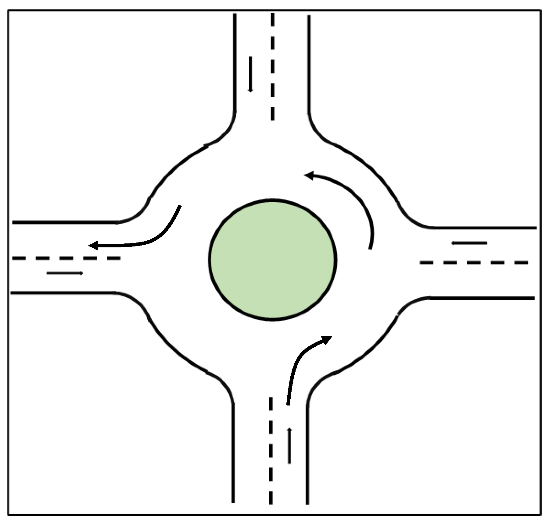
Figure 1. Diagram of a round intersection with arrows showing the allowed direction of travel.
Electronics 12 04670 g001
Figure 2. Diagram of the sequential decision-making problem.
Electronics 12 04670 g002
Figure 3. Diagram of two vehicles passing through the round intersection. Red and blue arrows show intersecting travel directions of two different vehicles.
Electronics 12 04670 g003
Figure 4. Diagram of reward (cost) for collision.
Electronics 12 04670 g004
Figure 5. Diagram of vehicle passing in round intersection (vehicles enter/exit the round intersection through the shaded areas, and the arrows show the direction of travel). The red arrows show entry and exit, and the green arrow shows following the round lane.
Electronics 12 04670 g005
Figure 6. The forward simulated path obtained using the state transition model directly. The large arrows show the direction of travel.
Electronics 12 04670 g006
Figure 7. Policy-based forward simulation.
Electronics 12 04670 g007
Figure 8. SUMO simulation environment.
Electronics 12 04670 g008
Figure 9. Two-vehicle scenario of passing the intersection.
Electronics 12 04670 g009
Figure 10. Multiple-vehicle scenario.
Electronics 12 04670 g010
Figure 11. Potential collision.
Electronics 12 04670 g011
Table 1. Simulation result of the 2-vehicle scenario.
DesciptionTotal RewardTotal Travel Time (s)Emergency Brake
OOPOMDP with policy-based state transition−527.921No emergency brake performed
OOPOMDP-based decision-making−593.67423Emergency brake performed by another vehicle
System driverNot applicable23Not applicable
Table 2. Simulation test result of the multiple-vehicle simulation.
DesciptionTotal RewardTotal Travel Time (s)Emergency Brake
OOPOMDP with policy-based state transition−45020.9No emergency brake performed
OOPOMDP-based decision-making−14,516.322Potential Collision
System driverNot applicable33.7Not applicable
Disclaimer/Publisher’s Note: The statements, opinions and data contained in all publications are solely those of the individual author(s) and contributor(s) and not of MDPI and/or the editor(s). MDPI and/or the editor(s) disclaim responsibility for any injury to people or property resulting from any ideas, methods, instructions or products referred to in the content.